Sage Journals: Discover world-class research

Abstract

The contact mechanism for joint surfaces is important for predicting the loading process and dynamic properties of precision machinery products. A multiasperity model considering the lateral interaction and coalescence of contact regions with oblique asperity contact, the interacting and coalescing Hertzian asperities (ICHA) model, is introduced in this work. Contact angle $α$ and radius of curvature $R (r)$ are vital parameters that are directly calculated based on grid points measured from the milling and grinding surfaces. Numerical simulations of $α$ and $R (r)$ were analysed. The results show that the proposed model is more effective at improving the contact area versus force relationship than various asperity models for low and middle contact forces. $α$ and $R (r)$ follow a Gaussian distribution. Because of the existence of coalescence, they decrease with increasing contact force. Furthermore, the $α$ and $R (r)$ in the startup phase are crucial data that can be used to judge the effects of oblique asperity contact. They are greatly influenced by fractal dimension $D$ and fractal roughness G. From the comparisons with the surfaces generated by Weierstrass-Mandelbrot function, it is suggested that to obtain an accurate contact prediction in the loading process, oblique contact is as important as lateral interaction and coalescence.

Keywords

Contact model oblique asperity discrete grid point contact angle radius of curvature

Introduction

The existence of joint surfaces between assemblies has enormous implications on the dynamic properties of precision machinery products.^1,2 The mechanism of contact action involves friction, wear, lubrication, adhesion, thermal conductivities and other contact statuses.^3–6 Many analytical methods have been proposed and improved to model machined surfaces. However, it is difficult to establish a complete, accurate and universal contact model owing to complex statuses in multiphysics. Most theoretical models are derived with some assumptions under given constraints and particular conditions.

The classical Hertz theory⁷ assumes that the deformation of the contact body is small and the relationship between the stress and strain is linear. The Greenwood–Williamson (GW) model⁸ is an asperity-based contact theory that treats the shape of the asperity as spherical or elliptical. The radius of curvature, size distribution and height distribution are defined and measurable. Fractal theory⁹ uses the self-similarity and self-affine characteristics of the machined surface and uses the size distribution of contact spots to follow the cumulative size distribution of islands. Wang and Komvopoulos¹⁰ improved the microcontact distribution function with a domain extension factor based on the continuous approximation of the Dirac delta function. Persson’s theory,¹¹ which deduces the surface separation and the contact pressure distribution from full contact to partial contact through boundary conditions, is practical and has grown popular in recent years. Based on these basic contact theories, in this study, many extended and modified versions are proposed, while some arguments are also raised that the conditions needed to obtain the exact relationship between the real contact area and load are harsh and restrictive. The interacting and coalescing Hertzian asperities (ICHA) approach has been shown to be extremely accurate at solving complex contact problems.

Yastrebov et al.¹² introduced a correction function and smoothing technique to deal with the contact boundary of a discrete mesh. The real contact area of a random rough surface can be calculated using this method. Putignano et al.¹³ found that the contact area is only related to the root mean square slope of the asperity height distribution. Numerical simulations also show that the relationship between the contact area and the load is nonlinear. Paggi and Ciavarella¹⁴ compared the accuracy of the coefﬁcient of proportionality $κ$ between the real contact area and load using various statistical theories, such as the Bush, Gibson and Thomas model and the GW model, using a range of generated fractal surfaces. The efficiency and accuracy can be signiﬁcantly improved by considering the interaction effects and simplifying the mesh discretisation method. Most related studies on contact mechanics focused on load, true contact area, surface separation, gap distribution, interfacial stress, multi-scale characteristics and related parameters of generated height proﬁles by Fourier transform.¹⁵ Moreover, few studies have introduced a detailed method that can measure and analyse real machined surfaces.

However, the micro-scale and nano-scale accuracy of precision equipment such as optical, capacitive, tomography and tactile probing systems have been greatly improved and are widely used. In addition, the reliability of data obtained from machined surfaces has been improved. Thus, it is reasonable and feasible to analyse real machined joint surfaces by measuring the surface point cloud. Bora et al.¹⁶ constructed a finite element numerical simulation model using surface data obtained via atomic force microscopy and estimated the relationship between the force and displacement of normal degrees of freedom using the Boussinesq solver. Campañá and Müser¹⁷ measured the surface morphology of refined steel via atomic force microscopy and calculated the area occupied by each atom using the Voronoi structure. The results showed that the contact pressure of randomly rough surfaces follows a Gaussian distribution, while the experimentally determined topographies obey an exponential distribution. The true contact area of the measured surface is 20% larger than that of the random surface. Putignano et al.¹⁸ regarded the effect between tire and pavement as being a grinding action that has fractal self-similar characteristics. The contour of the concrete pavement was measured by contact-less optical methods and compared with the surface generated by the power spectrum method. The variation of the limit contact area corresponding to the percolation threshold was analysed.

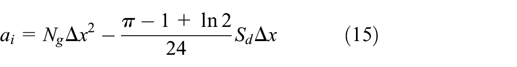
Some previous studies also found pronounced differences between real machined surfaces and generated random rough ones. One important reason is that the two rough surface contacts are usually assumed to be an elastic half-space or a rigid plane in contact with an isotropic rough surface (Figure 1(a)). However, the joint surfaces between real parts in precision machinery products usually have the same finish roughness. The oblique contact between asperities is unavoidable when the scales of the upper and lower rough surfaces are not significantly different (Figure 1(b)). The effect of oblique contact is simplified by various degrees or neglected except in cases involving friction, sliding and adhesion. However, it is clear from the visualisation and principle^19,20 that shoulder–shoulder contact between the asperities of rough surfaces is not only persistent but also exists on scales that differ from the amplified area in shown in Figure 1. Thus, a multi-scale analysis is necessary.

Figure 1.

Simplified surface contact between (a) rigid plane in contact with isotropic rough surface and (b) two rough surfaces with oblique contact asperities.

Sepehri and Farhang¹⁹ presented the normal and tangential load of single asperity based on the Hertz theory, in which the asperity height sum is assumed to be a Gaussian distribution. The minimum error of the total normal and tangential loads can reach 0.2%. However, the assumed Gaussian distribution was not verified, and the multi-step hybrid interactive and optimisation procedure was not clear. Jackson et al.²¹ described the average tangential and normal forces from the asperity interactions using semi-analytical and finite element simulations. The properties of typical metals were the study subjects to help verify their effectiveness. Mazeran and Beyaoui²² depicted the sliding of nanoscopic elastic contact under a scanning force microscope Si₃N₄ probe using an extended Hertz theory (Derjaguin, Muller and Toporov theory). The experimental results were in relatively good agreement with the Mindlin and Savkoor theories. Zhao et al.²³ extended the elastoplastic model considering the surface hardness proposed by Jackson and Green using the oblique contact condition. A white-light interferometer was used to measure the surface profile, and the asperity shape was fitted to an elliptical paraboloid. Because of the quadratic approximation of the radius of curvature and the offset of the intersection midpoint from the peak, the results still had a deviation error.

In this study, multiasperity contact analysis considering lateral interaction and the coalescence of contact regions is extended with oblique asperity contact. A suitable method was applied to the data clouds of two machined surfaces obtained by a three-coordinate measuring machine. As a result, a new method to calculate the contact angle and radius of curvature of the oblique contact point is discussed in detail. Contact stiffness measurement is used to indirectly verify the accuracy and efficiency of the proposed model and simulation method. Experimental data from milling and grinding surfaces were simulated and compared with generated topographies for qualitative analysis. The results show that the oblique contact can be considered to be the effect of interaction and coalescence, especially for low and medium loads on the machined surface. The fractal parameters play important roles in the contact angle and radius of curvature.

Model and theory

Contact model

In this work, frictionless non-adhesive contact was studied without considering sliding, wear and other mechanisms that occur in the tangential direction. Although oblique contact always has a tangential force, the normal force is the key behaviour. The material of the machined surface is homogenous. Asperity-based theory and Persson’s theory are the most commonly used surface contact theories.²⁴ Persson’s theory¹¹ is practical for adhesion, lubrication because the multi-scale and long-range elastic coupling properties enable the approximate process to obtain highly accurate simulation results. However, this theory extends the differential diffusion equation under full contact to partial contact without involving asperity topography. Asperity-based theory is a multi-asperity theory and has more advantages for situations of partial contact and low load. Various approaches have been introduced to consider the defects that may lead to significant errors. ICHAs were applied and extended to a newly proposed approach with oblique contact.

Figure 2 presents the geometric diagram of a single oblique asperity contact pair. In the contact model, the shape of the asperity is approximately elliptic paraboloid. The function of the contact force, $f_{a}$ , equivalent radius of curvature, $R (r)$ and asperity interference, $w$ , of the contact point can be given by the Hertz theory:

f_{a} = 4 E' R {(r)}^{0.5} w^{1.5} / 3

(1)

where $E'$ is the equivalent elastic modulus. According to the geometric relationships and derivative results of Sepehri and Farhang,¹⁹ the normal components can be obtained as

w = w_{n} \cos α

(2)

f_{n} = f_{a} \cos α

(3)

where $α$ is the contact angle, $w_{n}$ is the normal interference of the asperities and $f_{n}$ is the normal component of the contact force. The method¹⁹ proposed to calculate $R (r)$ uses the fourth-order approximation as $R (r) = R {(1 + r^{2} / R_{s}^{2})}^{1.5}$ , and $α$ can be given as $\cos α = {(1 + r^{2} / R_{s}^{2})}^{- 0.5}$ , in which $r_{1} = R_{1} r / R_{s}, r_{2} = R_{2} r / R_{s}, R_{s} = R_{1} + R_{2}$ , $R = (R_{1} + R_{2}) / R_{1} R_{2}$ , and $r_{1}$ , $R_{1}$ and $r_{2}$ , $R_{2}$ are the tangential deviations and radii of two summits, respectively. $R$ is the equivalent asperity radius for the contact of two hemispheres obtained by the arithmetic mean of the two principal radii. However, the elliptical contact patches are closer to the truth than the circular ones. Greenwood²⁰ demonstrated that the geometric mean value can obtain the plausible equivalent asperity radius of an elliptical solution with good approximation, which can be written as:

R = \sqrt{R_{1} R_{2}}

(4)

Figure 2.

(a) Single oblique asperity contact pair and (b) overlap region showing interferences in all directions.

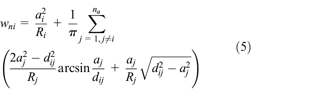
To consider the lateral interaction and coalescence of contact regions, the Interacting and Coalescing Hertzian Asperities (ICHA) multiasperity contact model proposed by Afferrante et al.²⁵ was applied to calculate the normal displacement, $w_{ni}$ , of a generic point in a non-contact region of asperity $AS P_{i}$ :

\begin{matrix} w_{ni} = \frac{a_{i}^{2}}{R_{i}} + \frac{1}{π} \sum_{j = 1, j \neq i}^{n_{a}} \\ (\frac{2 a_{j}^{2} - d_{ij}^{2}}{R_{j}} \arcsin \frac{a_{j}}{d_{ij}} + \frac{a_{j}}{R_{j}} \sqrt{d_{ij}^{2} - a_{j}^{2}}) \end{matrix}

(5)

where $a_{i}$ and $a_{j}$ are the ith and jth contact radii of asperities $AS P_{i}$ and $AS P_{j}$ , $R_{i}$ is the geometric mean of the principal radii of curvature, $d_{ij}$ is the tangential distance between asperities $AS P_{i}$ and $AS P_{j}$ , and $n_{a}$ is the total quantity of asperities. Meanwhile, two contact asperities for two surfaces are defined as a new asperity with equivalent contact radii $a_{eqv}$ , geometrical volume centroid, $(x_{eqv}, y_{eqv})$ and radius of curvature, $R_{eqv}$ , which can be given as:

a_{eqv}^{2} = a_{i}^{2} + a_{j}^{2}

(6)

x_{eqv} = (\frac{a_{i}^{4}}{R_{i}} x_{i} + \frac{a_{j}^{4}}{R_{j}} x_{j}) / (\frac{a_{i}^{4}}{R_{i}} + \frac{a_{j}^{4}}{R_{j}})

(7)

y_{eqv} = (\frac{a_{i}^{4}}{R_{i}} y_{i} + \frac{a_{j}^{4}}{R_{j}} y_{j}) / (\frac{a_{i}^{4}}{R_{i}} + \frac{a_{j}^{4}}{R_{j}})

(8)

R_{eqv} = \sqrt{R_{i}^{2} + R_{j}^{2}}

(9)

Radius of curvature based on grid points

One practical problem is that it is difficult to fit all asperities in real rough surfaces using elliptic paraboloids. Even if it works, the errors are great because the profile of the surface is composed of multi-scale asperities. Moreover, the valleys and peaks are determined by the machine tools and scratches. Surface defects are inevitable. Thus, the calculation method for the radius of curvature based on the profile of a real machined surface can reduce such errors and become more reliable.²⁶ The data of the profile are usually made up of discrete mesh points that coincide at regular intervals with differing normal interfacial separations.

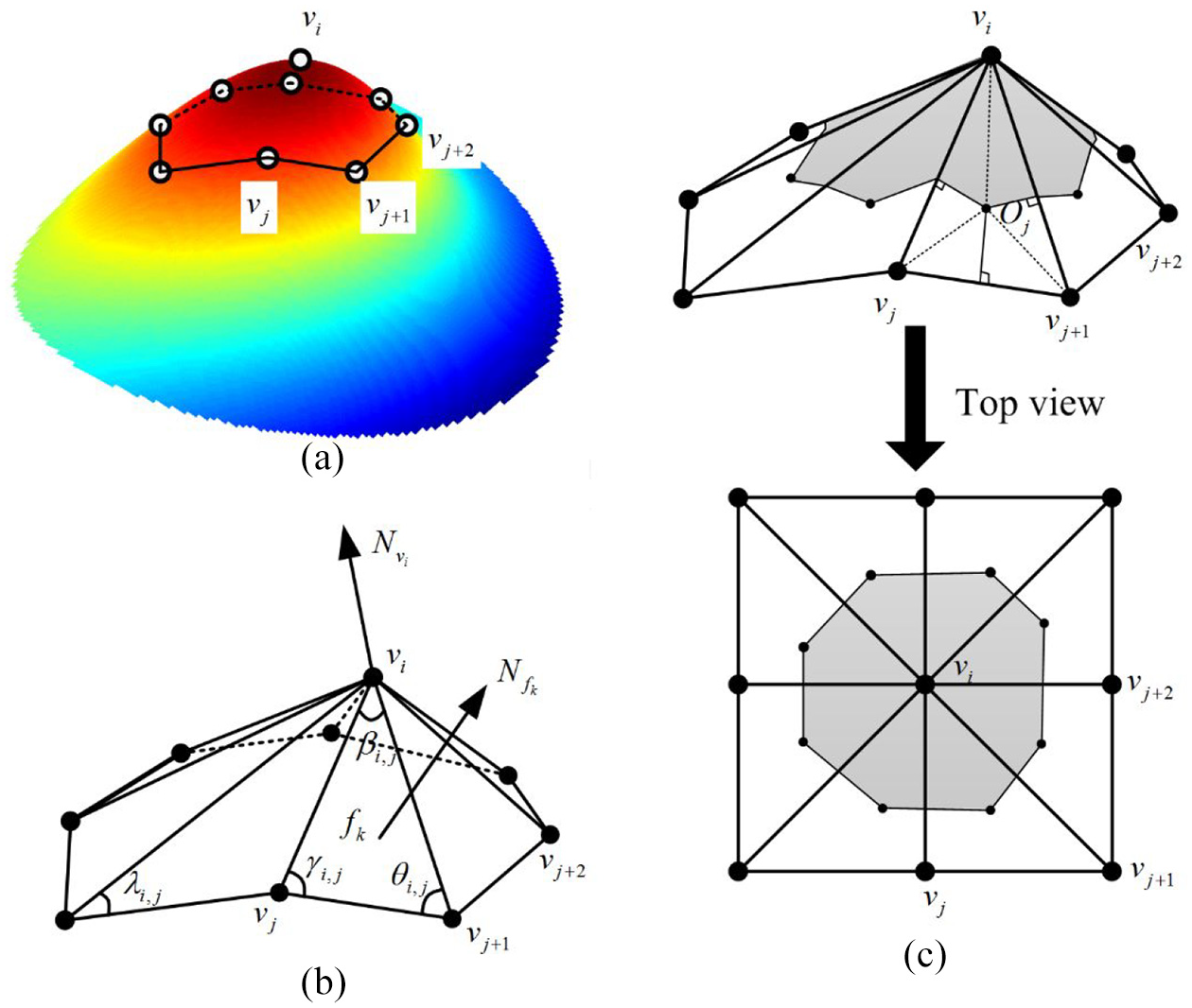
Figure 3(a) shows a three-dimensional (3-D) image of regular non-obtuse triangulated asperity $AS P_{i}$ meshes, where $v_{i}$ is the vertex and its 1-ring neighbours ${v_{j + k} : 0 \leq k \leq 7}$ . The unit length normal vector $N_{vi}$ of $v_{i}$ (Figure 3(b)) can be obtained as:²⁷

N_{vi} = \frac{\sum_{f_{k} \in F^{i}} | f_{k} | N_{f_{k}}}{‖ \sum_{f_{k} \in F^{i}} | f_{k} | N_{f_{k}} ‖}

(10)

where $F^{i}$ is the surface list of the triangle faces formed by $v_{i}$ and its 1-neighbourhood points, and $f_{k} (1 \leq k \leq 8)$ is a 3-D triangle face belonging to $F^{i}$ . $N_{f_{k}}$ is the unit length normal vector for each face. The area $| f_{k} |$ is treated as the weighting coefficient introduced by Taubin. ‖‖ means norm operation. Vector angle, centroid and triangle geometrical features also affect the normal vector, and many studies have proposed improved algorithms. Because the precision profiler can achieve uniform space sampling and the machined surface has regular textures and patterns, the accuracy of the surface area is sufficient to be the weighting coefficient.

Figure 3.

(a) 3-D image of regular non-obtuse triangulated asperity, (b) diagram of different parameters in the discrete grid and (c) Voronoi region and its top view.

There are several classical methods of discrete curvature estimation based on grid surfaces, such as tensor-based techniques, derivative methods with local quadric approximation and mathematical formulae based on operators.²⁸ Meyer et al.²⁹ introduced a ﬂexible tool that approximates arbitrary triangle meshes by averaging Voronoi cells. This method is applied to calculate the equivalent radius of curvature $R (r)$ of the contact point in equation (1) directly without the tangential deviations and fitting process of the asperity shape. However, $R (r)$ is the radius of the mean curvature rather than the radius of the normal curvature, principal curvature or Gaussian curvature. The grey parts in Figure 3(c) depict top view of the Voronoi region for a vertex with $v_{i}$ and the neighbours $v_{j}$ . $O_{j}$ is the circumcentre of face $f_{k}$ . The non-obtuse Voronoi area $A_{Vori, j}$ in triangle $Δ v_{i} v_{j} v_{j + 1}$ and the total Voronoi area $A_{Vori}$ of $v_{i}$ can be given as:

A_{Vori, j} = \frac{1}{8} ({‖ \bar{v_{j} - v_{i}} ‖}^{2} \cot ∠ θ_{i, j} + {‖ \bar{v_{j + 1} - v_{i}} ‖}^{2} \cot ∠ γ_{i, j})

(11)

A_{Vori} = \frac{1}{8} \sum_{j = 1}^{n} (\cot θ_{i, j} + \cot λ_{i, j}) ‖ \bar{v_{j} - v_{i}} ‖^{2}

(12)

where $n$ is the amount of face $f_{j}$ and $β_{i, j}$ , $γ_{i, j}$ , $θ_{i, j}$ and $λ_{i, j}$ are the angles between vectors, as shown in Figure 3(b). In addition, $A_{Vori, j} = 0.5 * A_{Δ v_{i} v_{j} v_{j + 1}}$ if $β_{i, j}$ is an obtuse angle, and $A_{Vori, j} = 0.25 * A_{Δ v_{i} v_{j} v_{j + 1}}$ if $γ_{i, j}$ or $θ_{i, j}$ is an obtuse angle. The radius of the mean curvature $R_{i}$ of the asperity $AS P_{i}$ and equivalent radius of curvature $R (r)$ can be obtained by equation (4) as:

R_{i} = \frac{4 A_{Vori}}{\sum_{j = 1}^{k} (\cot θ_{i, j} + \cot λ_{i, j}) (\bar{v_{j} - v_{i}}) N_{vi}}

(13)

R (r) = \sqrt{R_{1 i} R_{2 i}}

(14)

Where $R_{1 i}$ and $R_{2 i}$ are the radii of the mean curvature of the two asperities at the contact point, as shown in Figure 2(b).

Contact area and contact angle

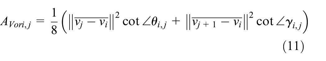
Although the contact region of the oblique contact has a slope, the contact area from the projection view is treated as the true contact area. Figure 4(a) describes a 3-D mesh of arbitrary asperity $AS P_{i}$ , in which the grey zone is the contact region. The contact area extracted from the coarse grid can be computed simply by counting the number of grid points $N_{g}$ . Each point contributes an area, $Δ x^{2}$ , where $Δ x$ is the grid side length. The nominal contact area is $a_{i} = N_{g} Δ x^{2}$ . From the top view in Figure 4(b), $a_{i}$ there are significant errors because the interface contact points are in partial contact rather than full contact. Yastrebov et al.³⁰ introduced a useful corrective factor to compensate for this deviation by:

a_{i} = N_{g} Δ x^{2} - \frac{π - 1 + \ln 2}{24} S_{d} Δ x

(15)

where $S_{d} = M Δ x$ is the perimeter of the contact/non-contact boundaries and $M$ is the number of switches from contact to non-contact and vice versa along grid points both in the vertical and horizontal directions, as shown by the red line in Figure 4(b).

Figure 4.

(a) 3-D meshes of arbitrary asperity and (b) top view of contact zones on a coarse grid.

As mentioned, $\cos α = {(1 + r^{2} / R_{s}^{2})}^{- 0.5}$ can be used to calculate the contact angle. However, for real profiles measured by the machined surface, it is difficult to obtain $r$ and other tangential deviations for the same reason that it is difficult to obtain the radius of curvature $R_{i}$ . Figure 5 is the left view of Figure 4(a), and it presents the deformation of a single asperity with oblique contact. Grid points B $(x_{B}, y_{B})$ and D $(x_{D}, y_{D})$ are the crossover points of the contact boundaries and the curve between summit A and contact point C corresponding to the position in Figure 4(a). Thus, the contact angle $α$ can be calculated between the angle of BD and substrate as follows:

\tan α = (y_{B} - y_{D}) / (x_{B} - x_{D})

(16)

Figure 5.

Deformation of single asperity with oblique contact.

Measurement and simulation

Surface measurement and data processing

Precision instruments, such as atomic force microscopy (AFM), scanning force microscopy (SFM) and surface force apparatus (SFA) optical, capacitive, tomography and tactile probing systems, are becoming more and more accurate at surface measurement.³¹ A three-coordinate measuring machine (ACCURA II AKTIV, Carl Zeiss AG, GER) was used to measure the surface topography, as shown in Figure 6. Four samples formed by milling and grinding forming methods were selected as the upper and lower joint surfaces. The sample material was C45E4 (ISO) steel. To take the effect of the fixture, machine tool and processing strain into consideration, four test areas (1–4) of each sample were collected to compare and optimise the measured data, as shown in Figure 6. The holes were utilised as the benchmark to calibrate the position of the test areas. The sample size was 20 × 20 mm, and the test area was 5 × 5 mm. The sample interval $Δ x$ was 50 μm, and the measurement resolution was 2 μm.

Figure 6.

Experimental equipment and samples.

It is necessary to process the measured data with random errors, systematic errors and noise. Amongst these, systematic errors can be ignored because the relative positions of the data points remain unaffected. Furthermore, the flatness and parallelism of the upper and lower surfaces were analysed to correct the deflection. For random errors and noise, general data processing methodology is not appropriate. When these errors are reduced, the multi-scale features are also removed. The wavelet-based method is feasible for machined surface denoising.³² By decomposing and reconstructing the measured data, the noise can be reduced by setting low-pass and high-pass frequency thresholds at different levels. However, because the measurement interval is still large relative to the size of asperity, it is generally difficult to continuously take a plurality of points on an asperity slope. The surface obtained is zigzag, and the asperity is tapered. To compute the parameter of oblique contact for a smooth asperity surface, data interpolation is required.³³ Detailed illustrations of wavelet denoising and data interpolation are not outlined in this work as they can be implemented easily .

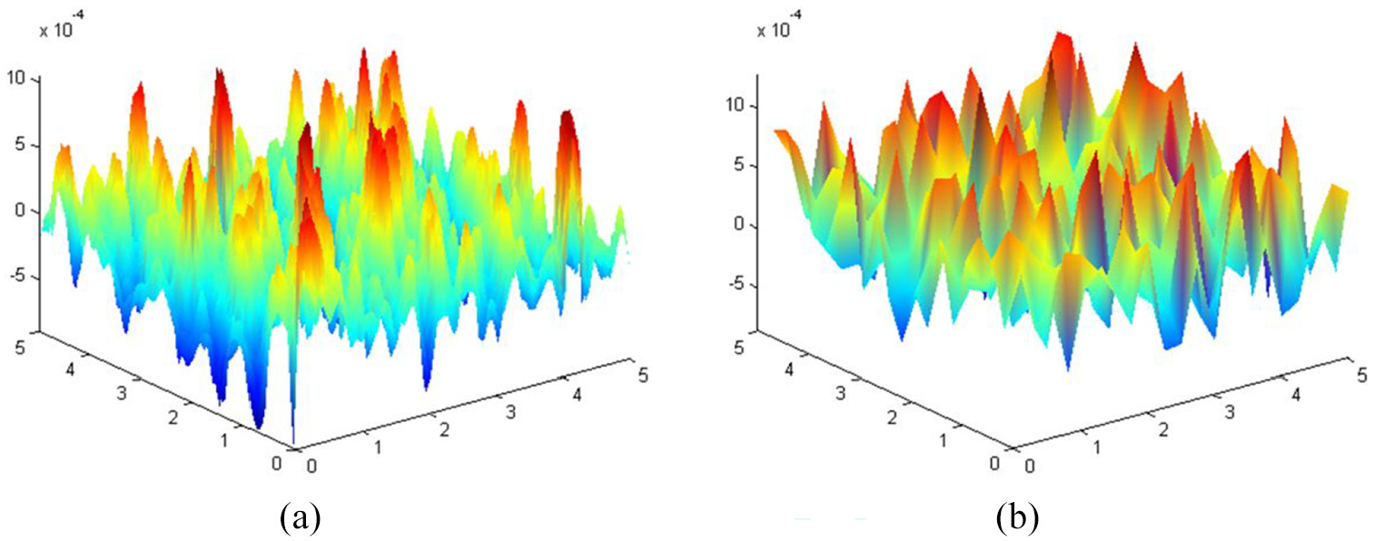
Because machined surfaces usually have multi-scale and self-similar profiles^34,35 fractal dimension $D$ and fractal roughness $G$ were used to quantify the surface features. The fractal parameters of each sample are evaluated using the structure function (SF) method, which can obtain a good result for two-dimensional fractal dimensions $D_{f} (D = D_{f} + 1)$ and $G$ compared to methods of the same type.³⁶ For the milling surface, $D = 2.5$ and G = 3.0 × 10⁻⁵ mm, and $D = 2.6$ and G = 6.5 × 10⁻⁴ mm for the grinding surface. Figures 7(a) and 8(a) present 3-D images of the milling and grinding surface profiles.

Figure 7.

3-D images of profiles with same parameters: (a) milling surface profile and (b) surface proﬁle generated by WM function.

Figure 8.

3-D image of profiles with same parameters: (a) grinding surface profile and (b) surface proﬁle generated by WM function.

Surface profiles generated by WM function

Regenerated surfaces are used to evaluate the relationship between the fractal parameters and the characteristics of the oblique contact. Multi-scale and fractal profiles can be synthesised using many techniques, such as the Fourier transform ﬁltering algorithm with prescribed Hurst exponent or power spectrum density, the Weierstrass-Mandelbrot (WM) function method and the midpoint displacement method.^37,38 The surface height function $z (x, y)$ of the 3-D fractal surfaces generated by the WM function method is composed of simultaneous sinusoidal equations. A modified WM function can be given as

\begin{matrix} z (x, y) = L {(\frac{G}{L})}^{D - 2} {(\frac{\ln γ}{M})}^{0.5} \sum_{m = 1}^{M} \sum_{n = 0}^{n max} γ^{(D - 3) n} [\cos ϕ_{m, n} - \\ \cos {\frac{2 π γ^{n} {(x^{2} + y^{2})}^{0.5}}{L} \cos [\tan^{- 1} (\frac{y}{x}) - \frac{π m}{M}] + ϕ_{m, n}}] \end{matrix}

(17)

where $x$ and $y$ are the planar Cartesian coordinates, $L$ is the sample length, $γ$ is a scale parameter that is, usually set at 1.5, $M$ is the number of superposed ridges, $ϕ$ is a random phase and $n$ ( $n max$ is the upper limit) is a frequency index. Figures 7(b) and 8(b) show the surface profiles generated by the WM function with the same fractal parameters as those of the milling and grinding surfaces. The asperities of real machined surfaces are smoother, while the shapes of asperity are similar to those of the cone for the generated surfaces. Furthermore, it has been pointed out that the WM function has some limitations.^35,39 For instance, the approximate continuous power spectrum contains limited bandwidth, which means that the function can generate limited characteristics of specific scales. Some studies also found that the regenerated proﬁles based on the self-afﬁne WM function are not consistent with the machined real surface proﬁles.³⁵ However, this function can reflect the variation trend between the fractal parameters and contact mechanics to some extent. Thus, the WM function is sufficient for reliable qualitative analyses.

Procedure for numerical simulation

Figure 9 shows the contact procedure of two surfaces. The $x$ and $y$ coordinates of the data points in lower surface $S_{l}$ and upper surface $S_{u}$ are initially fixed with $z$ coordinates $z_{u} > z_{l}$ $(z_{u} \in S_{u}, z_{l} \in S_{l})$ . The contact iterative operation is the downward displacement of $z_{u}$ with a fixed $z_{l}$ . When $z_{u} > z_{l}$ , the asperity pair begins to contact. Before the iteration, some data need to be calculated, including the coordinates and radii of curvature $R (r)$ of the initial contact points of all asperity contact pairs, $P A_{i} {(lAS P_{i}, uAS P_{ui}) : lAS P_{i} \in S_{l}, uAS P_{i} \in S_{u}, 0 < i \leq n_{a}}$ , using equations (13) and (14). After that, the surface $S_{u}$ starts to descend step by step as $z_{u (next)} = z_{u} - Δ z$ according to the height gap, $Δ z$ which can be arranged by the values of $z_{u}$ . The overall procedures of each step to simulate contact asperity pair $P A_{i}$ of the upper and lower surface proﬁles are detailed as follows.

(1) $a_{i}$ and $α$ of $P A_{i}$ can be calculated using equations (15) and (16) if $w_{n} > 0 (z_{u} < z_{l})$ . Otherwise, consider the next asperity pair, $P A_{i + 1}$ .

(2) Determine contact areas $a_{i}$ for all asperity pairs $P A_{j}$ using equation (15). if $a_{j} > 0$ , asperity pair $P A_{j}$ contributes to $w_{n}$ .

(3) (a) If $j = i$ , it means that $P A_{i}$ is the first contact pair on the surface without lateral interaction, and the contribution to $w_{n}$ is $a_{i}^{2} / R_{i}$ .

(b) If $j \neq i$ and there is no overlap between $P A_{i}$ and $P A_{j}$ , $P A_{j}$ contributes to $w_{n}$ is given by the term in the brackets in equation (5).

(c) If $j \neq i$ and there is overlapping between $P A_{i}$ and $P A_{j}$ , it means that $lAS P_{i}$ and $lAS P_{j}$ coalesce in contact spots. Thus, they are replaced by a new asperity with $a_{eqv}$ , $(x_{eqv}, y_{eqv})$ , and $R_{eqv}$ by equations (6)–(9). Then, return to Procedure 1.

(4) Calculate $f_{n}$ using equations (1)–(3) and (5).

Figure 9.

The contact procedure of two surfaces.

Through these procedures, the total normal force $F_{n}$ and total real contact area $A_{n}$ for each step can be obtained by $F_{n} = \sum_{i = 1}^{n_{a}} f_{n}$ and $A_{n} = \sum_{i = 1}^{n_{a}} a_{i}$ . Moreover, the distribution of contact angle $n (α)$ , distribution of contact radius $n (R)$ , total real contact area fraction $A_{n} / A_{a}$ and distribution of contact clusters can be determined, where A_a = 5 × 5 mm is the apparent area of the contact region. The dimensionless total normal contact force $F_{n}^{*}$ can be given by

F_{n}^{*} = F_{n} / E' A_{a}

(18)

Results and discussion

Contact area

To demonstrate the accuracy of the contact area evaluation by the proposed model, which is the modified version of ICHA (m-ICHA), the total real contact area fraction $A_{n} / A_{a}$ and dimensionless total normal contact force $F_{n}^{*}$ relative to different contact models are plotted in Figure (10) by averaging the four pairs of different test areas in milling and grinding surfaces. The model (IHA), which considers elastic coupling, was introduced by Ciavarella et al.⁴⁰ Some studies have already found that the ICHA model is the most accurate model. From results relative to GW, IHA, ICHA and m-ICHA models, it also reveals that the ICHA model can obtain good results and it is critically essential to lateral interaction and coalescence of contact regions. Otherwise, the area versus load relation would be predicted with poor accuracy, as shown for the GW and IHA models. Furthermore, the results of the m-ICHA model are not in perfect agreement with those of the ICHA model, especially when $F_{n}^{*} < 0.3$ . The results of the milling surface are clearer. Evidently, the effect of oblique asperity contact leads to bias. Equations (1)–(3) yield:

f_{n} = 4 {(\cos α)}^{0.5} E' R {(r)}^{0.5} w^{1.5} / 3,

(19)

which shows that the contact angle $α$ and radius of curvature $R (r)$ are vital influence coefficients. Generally, $α \leq 1$ , and the $R (r)$ of the slope is larger than that of the summits of the same asperity pair. Under the comprehensive effect of both coefficients, the bias becomes smaller and almost equals zero with increasing contact force. This exhibits that the contact model for oblique contact can lead to more accurate results.

Figure 10.

Real contact area fraction $A_{n} / A_{a}$ with dimensionless total normal contact force $F_{n}^{*}$ relative to different contact models: (a) milling surface and (b) grinding surface.

Contact angle

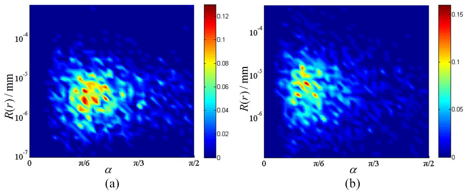
Figure 11 shows the joint distribution of contact angle $α$ and real contact area fraction $A_{n} / A_{a}$ for milling and grinding surfaces, and the insets the amplified regions of $A_{n} / A_{a} \subset [0, 0.3]$ . Because of the existence of coalescence in equations (6)–(8), contact spots can merge forming contact patches. The contact angle $α$ becomes smaller (the amount of contact pairs with big $α$ decreases relatively) with the increase in contact area. For arbitrary $A_{n} / A_{a}$ , $α$ presents a Gaussian-like distribution, and its mean value and variance decrease rapidly until $A_{n} / A_{a} \approx 0.6$ . Moreover, the $α$ of the grinding surface is almost equal to zero, corresponding to the overlapping of the ICHA and m-ICHA models in Figure 10(b). This suggests that the oblique contact asperity pair almost vanishes when the contact area is large enough.

Figure 11.

Joint distribution of contact angle $α$ and real contact area fraction $A_{n} / A_{a}$ : (a) milling surface and (b) grinding surface.

However, coalescence plays a very important role in the contact mechanism. In particular, for low and middle contact forces, a large number of micro-asperities that exist in a macro-asperity region gradually become part of the macro-asperity. Finally, the dominant macro-asperities are almost turned into the base of the surface. Seen in another light, this explains that the oblique contact takes effect mainly in the low and middle contact forces.

Radius of curvature

The results are presented for the joint distribution of the radius of curvature $R (r)$ and real contact area fraction $A_{n} / A_{a}$ , as shown in Figure 12. Equation (9) indicates that $R (r)$ also increase with an increase in the contact area. The distribution of $R (r)$ is also Gaussian-like for an arbitrary $A_{n} / A_{a}$ . Its mean value undergoes a slight change in the logarithmic coordinate, while the variance of the trend becomes much smaller in processes. The distribution width of the milling and grinding surfaces is almost the same, while the distribution of the grinding surface is more concentrated. This is because the fractal dimension $D$ on the grinding surface is larger, which means that the ratio of micro-asperities is larger. Although the fractal roughness $G$ of the grinding surface is larger, its effect is much slighter. Some approaches³⁵ also observed that fractal roughness $G$ depends on fractal dimension $D$ , so it is meaningless to discuss $G$ without $D$ .

Figure 12.

Joint distribution of radius of curvature $R (r)$ and real contact area fraction $A_{n} / A_{a}$ : (a) milling surface and (b) grinding surface.

The comprehensive analysis of Figures 10 to 12 indicates that lateral interaction and the coalescence of contact regions can lead to definitive improvement of the contact model. The oblique asperity contact can also further enhance the prediction accuracy, especially for low and middle contact forces. Under practical circumstances, it is difficult to reach a value of one for real contact area fraction $A_{n} / A_{a}$ for the machined joint surfaces. Hence, taking full consideration of the oblique asperity contact with contact angle $α$ and radius of curvature $R (r)$ can optimise the loading process.

Initial contact angle and radius of curvature

From the above conclusions, it is clear that contact angle $α$ and radius of curvature $R (r)$ in the startup phase seem to be the crucial points that can judge the effect of oblique asperity contact. Since the $A_{n} / A_{a}$ , $α$ and $R (r)$ of the grinding surface tend to stabilise more quickly, as shown in Figures 10 to 12, it can be deduced that the deviation ratio of the mean value has a direct relationship with the variability rate of the contact area. Fractal dimension $D$ and fractal roughness $G$ represent the multi-scale characteristics of machined rough surfaces. Hence, the profiles generated by the WM function were simulated to explore the comparison with different fractal parameters.

The value range of the fractal dimension $D$ is defined as $2 < D < 3$ . However, previous studies have shown that the $D$ of real machined surfaces is only possible in a particular range. For instance, Persson⁴¹ found out that $D$ is usually $< 2.3$ for polished or sandblasted surfaces by the power spectral density (PSD) method. Zhang et al.³⁶ demonstrated that such results occur when nominally self-similar real rough surfaces are assumed to be self-affined. The PSD method may not provide an adequate approach for real surfaces, while the SF method can be regarded as a reliable one of various methods. In the present work, ${D : 2.4, 2.5, 2.6}$ is set as the simulation variable according to the fractal parameters of the measured milling and grinding surfaces.

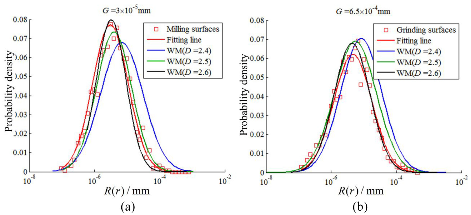
Figure 13 presents the probability density as a function of contact angle $α$ for G = 3 × 10⁻⁵ mm (Figure 13(a)) and G = 6.5 × 10⁻⁴ mm (Figure 13(b)). The results were obtained by averaging on eight different measured and numerically generated surfaces. The proposed comparison makes clear that fractal parameters have a tremendous influence on the initial $α$ . The probability density distribution of generated surfaces is well described by Gaussian distribution. Measured surfaces do not strictly obey Gaussian distribution and are not in good agreement with the generated surfaces for the same fractal parameters, especially for $α > π / 4$ . Close observation reveals that the mean values of measured surfaces are smaller. Furthermore, the distribution for smaller $D$ and bigger $G$ is much closer to zero with a smaller variance.

Figure 13.

Probability density of initial contact angle $α$ with measured and generated surfaces for various $D$ values: (a) G = 3 × 10⁻⁵ mm and (b) G = 6.5 × 10⁻⁴ mm.

In addition, the contact angle $α$ of the oblique contact for elliptic parabolic asperities should be $0 \leq α < π / 4$ ,⁴² but it was $α > π / 4$ in the numerical simulations, as presented in Figure 13. This contradiction is caused by the theoretical error that the rough surfaces are fitted by discrete grid points at regular intervals $Δ x$ . The grids in Figure 14 depict different length scale asperity pairs obtained from the same surface. The small length-scale asperity corresponds to $Δ x$ , which is determined by the resolution of the instrument and the sampling interval of the simulation. In this case, the transition curve is replaced with a straight line, and the shape of the elliptic parabolic asperity is turned into a cone. Hence, somewhere in the surface occurs as a contact pair with $α > π / 4$ . Irrespective of the small $Δ x$ , the asperities shown in Figure 14(b) are always existential owing to the multi-scale characteristics of the machined surface. Moreover, almost all initial contact angles $α$ of the black line in Figure 14(a) are $> π / 4$ . This indicates that most asperity scales on the generated surface are almost approximate with the interval in the startup phase when $D = 2.6$ and G = 3 × 10⁻⁵ mm. Thus, it can be concluded that there are some limitations in analysing the proposed contact model based on measured grid points: the accuracy of the simulation is constrained by the resolution of the instrument at very low contact forces. This is one of the main criticisms of asperity-based contact theory.

Figure 14.

Grids of oblique contact asperity pairs at same interval: (a) large length-scale and (b) small length-scale.

Figure 15 shows the probability density for the initial radius of curvature $R (r)$ . Similarly, the distribution of probability density versus the $R (r)$ relationship follows the Gaussian distribution, and a larger $D$ results in a smaller $R (r)$ . Compared with contact angle $α$ in Figure 13, the differences amongst $R (r)$ of various fractal parameters are smaller. Actually, $α$ and $R (r)$ are not completely independent. When $α$ converges towards zero, the contact point is near the summit and $R (r)$ is noticeably close to the radius of curvature for the summit, which is the smallest in the asperity. However, this dependency is strong only for a small $α$ . As shown in Figure 16, the joint distribution of $R (r)$ and $α$ corresponds to their distribution in Figures 13 and 15, respectively. And $R (r)$ and $α$ appear to be mutually independent.

Figure 15.

Probability density of initial radius of curvature $R (r)$ with measured and generated surfaces for various $D$ values: (a) G = 3 × 10⁻⁵ mm and (b) G = 6.5 × 10⁻⁴ mm.

Figure 16.

Joint distribution of contact angle $α$ and radius of curvature $R (r)$ in the startup phase: (a) milling surface and (b) grinding surface.

Contact stiffness experimental verification

Direct measurement of contact area, contact angle and radius of curvature is difficult. Therefore, contact force and contact stiffness of the samples are taken as the indirect variates to verity the theory.

The data of the contact stiffness experiment in Zhang et al.⁴² is utilized. The distribution of contact angle is assumed as Gaussian distribution and uniform distribution simply. The values of parameter $c_{i}$ are given as ${1, 1.1, 1.2 \dots 1.8, 1.9}$ where $c_{i}$ is an intermediate variable and $\cos α_{i} = {(1 + r^{2} / R_{s}^{2})}^{- 0.5} = c_{i}^{- 0.5}$ . For uniform distribution, $A_{i} / A_{n} = {0.1, 0.1, 0.1 \dots 0.1, 0.1}$ . And for Gaussian distribution, when $c_{i} = 1.1$ is set as the average point and the standard deviation is given as 0.4, the contact area ratio is $A_{i} / A_{n} = {0.2, 0.18, 0.16, 0.14, 0.1, 0.08, 0.06, 0.035, 0.025, 0.02}$ . Obviously, these assumptions caused enormous errors as shown in Figures 13 and14⁴².

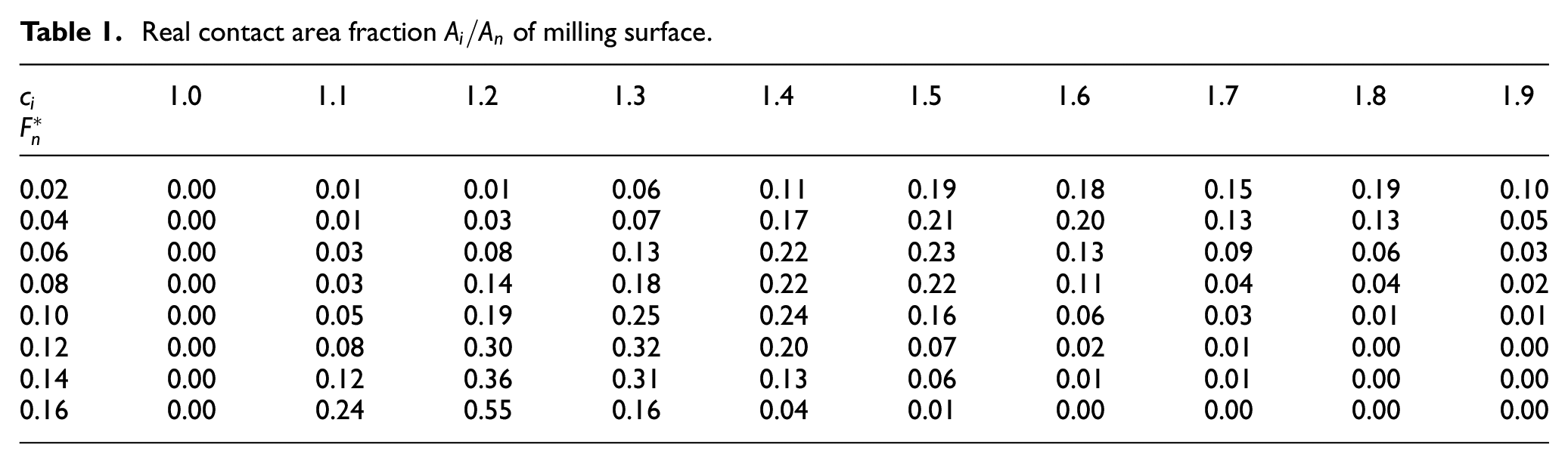
Based on the procedure for m-ICHA numerical simulation proposed in the paper, we can obtain accurate $A_{i} / A_{n}$ as listed in Tables 1 and 2. Figures 17 and 18 show the dimensionless normal stiffness and the errors of experiment, simulations of the modified WK models with different size distributions (Gaussian distribution, uniform distribution and the simulated distribution).

Table 1.

Real contact area fraction $A_{i} / A_{n}$ of milling surface.

$c_{i}$ $F_{n}^{*}$	1.1	1.2	1.3	1.4	1.5	1.6	1.7	1.8	1.9
0.02	0.01	0.01	0.06	0.11	0.19	0.18	0.15	0.19	0.10
0.04	0.01	0.03	0.07	0.17	0.21	0.20	0.13	0.13	0.05
0.06	0.03	0.08	0.13	0.22	0.23	0.13	0.09	0.06	0.03
0.08	0.03	0.14	0.18	0.22	0.22	0.11	0.04	0.04	0.02
0.10	0.05	0.19	0.25	0.24	0.16	0.06	0.03	0.01	0.01
0.12	0.08	0.30	0.32	0.20	0.07	0.02	0.01	0.00	0.00
0.14	0.12	0.36	0.31	0.13	0.06	0.01	0.01	0.00	0.00
0.16	0.24	0.55	0.16	0.04	0.01	0.00	0.00	0.00	0.00

Table 2.

Real contact area fraction $A_{i} / A_{n}$ of grinding surface.

$c_{i}$ $F_{n}^{*}$	1.0	1.1	1.2	1.3	1.4	1.5	1.6	1.7	1.8	1.9
0.02	0.01	0.06	0.06	0.14	0.23	0.15	0.10	0.10	0.06	0.09
0.04	0.02	0.10	0.13	0.18	0.19	0.14	0.09	0.07	0.04	0.04
0.06	0.02	0.14	0.20	0.20	0.18	0.09	0.07	0.04	0.03	0.03
0.08	0.05	0.18	0.24	0.21	0.15	0.07	0.04	0.02	0.02	0.02
0.10	0.07	0.25	0.29	0.20	0.09	0.04	0.02	0.01	0.01	0.02
0.12	0.11	0.35	0.32	0.14	0.04	0.03	0.00	0.00	0.00	0.01
0.14	0.16	0.42	0.28	0.08	0.03	0.02	0.00	0.00	0.00	0.01
0.16	0.30	0.51	0.16	0.02	0.01	0.00	0.00	0.00	0.00	0.00

Figure 17.

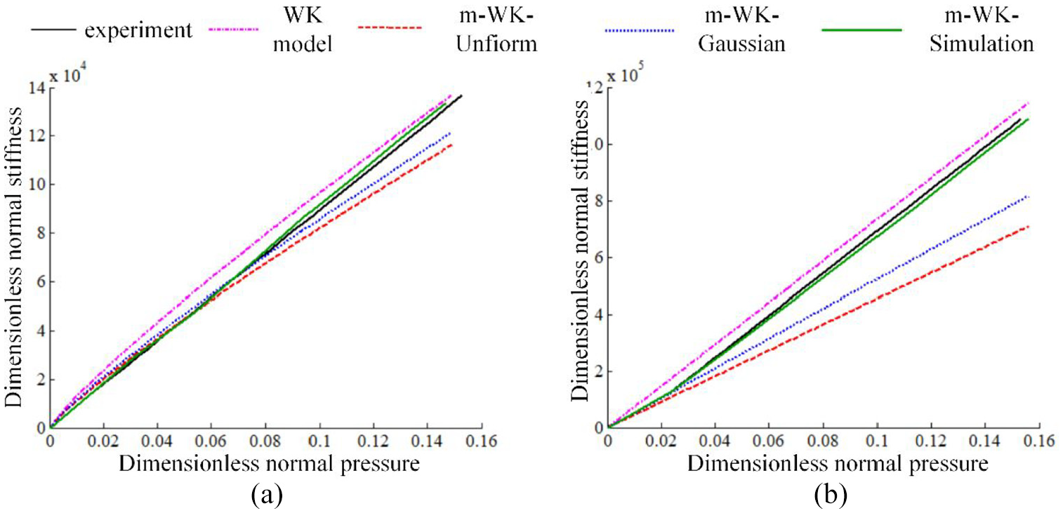
Comparison of dimensionless normal stiffness by experiment results and fractal models: (a) milling surface and (b) grinding surface.

Figure 18.

Errors of dimensionless normal stiffness between experiment results and fractal models: (a) milling surface and (b) grinding surface.

Combined with the discussion in Zhang et al.⁴² the dimensionless normal pressure and the dimensionless normal stiffness of milling surface and grinding surface are calculated based on the simulated distribution of Real contact area fraction $A_{i} / A_{n}$ . It can be seen from the figures that in the entire process, the stiffness is almost in line with the actual experiment results and the variance is small. The maximum errors of Gaussian distribution and uniform distribution reach more than 10% while the errors of the simulated distribution are less than 5%. Especially during the light load process between the milling surfaces, the accuracy is improved by more than two times. Moreover, the both errors for milling and grinding surfaces are less than 5% which shows that the simulation can reflect the actual contact principles of machined rough surfaces.

Thus, it can be summarized that the modified WK model considering the oblique contact can achieve accurate prediction of the dimensionless normal stiffness when the distributions between contact force, contact angle $α$ and real contact area fraction $A_{i} / A_{n}$ are estimated precisely. And it also verified the correctness of the proposed model in the paper.

Conclusion

We analysed the contact characteristics of real machined rough surfaces by extending a multiasperity model considering lateral interaction and the coalescence of contact regions with oblique asperity contact. Numerical simulations were applied with directly calculated contact angles $α$ and radii of curvature $R (r)$ based on grid points. The prediction abilities of the proposed method were assessed. Compared with several contact models, the contact area evaluation of the suggested model can lead to more accurate results, especially at low loads. The contact angle $α$ and radius of curvature $R (r)$ are vital contact parameters that are affected by coalescence in the loading process. Both follow a Gaussian distribution and decrease with an increase in the contact force. Furthermore, the rate of the reduction is influenced by $α$ and $R (r)$ in the initial state. The effect of oblique contact is less with a smaller fractal dimension $D$ and larger fractal roughness $G$ , as seen from the comparisons with the measured surfaces and generated surfaces by the WM function. However, the joint surfaces of precision machinery parts usually have relatively large $D$ and small $G$ values. Based on the contact stiffness experiment, the accuracy and efficiency of the proposed model and simulation procedure are verified. Thus, to accurately predict the loading process, it is essential to take oblique contact, lateral interaction and coalescence into consideration.

Footnotes

Acknowledgements

The authors would like to thank Prof. Guoxi Li and Assoc. Prof. Meng Zhang for suggestions.

Handling Editor: James Baldwin

Declaration of conflicting interests

The author(s) declared no potential conflicts of interest with respect to the research, authorship, and/or publication of this article.

Funding

The author(s) received no financial support for the research, authorship, and/or publication of this article.

ORCID iD

Kai Zhang

References

Wan

Gong

, et al. An improved algorithm for the normal contact stiffness and damping of a mechanical joint surface. Proc Inst Mech Eng Part B J Eng Manuf 2014; 228: 751–765.

Zhai

Huang

, et al. Investigation of the contact performance of machined surface morphology. Tribol Int 2017; 107: 125–134.

Pan

Wang

, et al. A normal contact stiffness fractal prediction model of dry-friction rough surface and experimental veriﬁcation. Eur J Mech Solid 2017; 66: 94–102.

Zou

Wang

. Investigation of the contact stiffness variation of linear rolling guides due to the effects of friction and wear during operation. Tribol Int 2015; 92: 472–484.

Sudeep

Tandon

Pandey

. Vibration studies of lubricated textured point contacts of bearing steels due to surface topographies: Simulations and experiments. Tribol Int 2016; 102: 265–274.

Anciaux

Molinari

. A molecular dynamics and ﬁnite elements study of nanoscale thermal contact conductance. Int J Heat Mass Trans 2013; 59: 384–392.

Johnson

. Contact mechanics. Cambridge: Cambridge University Press, 1985.

Greenwood

Williamson

. Contact of nominally flat surfaces. Proc R Soc Lond A 1966; 295: 300–319.

Majumdar

Bhushan

. Fractal model of elastic-plastic contact between rough surfaces. J Tribol 1991; 113: 1–11.

10.

Wang

Komvopoulos

. A fractal theory of the interfacial temperature distribution in the slow sliding regime: part I-elastic contact and heat transfer analysis. J Tribol 1994; 116: 812–823.

11.

Persson

BNJ

. Elastoplastic contact between randomly rough surfaces. Phys Rev Lett 2001; 87: 116101.

12.

Yastrebova

Anciaux

Molinari

. On the accurate computation of the true contact-area in mechanical contact of random rough surfaces. Tribol Int 2017; 114: 161–171.

13.

Putignano

Afferrante

Carbone

, et al. The inﬂuence of the statistical properties of self-afﬁne surfaces in elastic contacts: a numerical investigation. Mech Phys Solids 2012; 60: 973–982.

14.

Paggi

Ciavarella

. The coefﬁcient of proportionality

κ

between real contact area and load, with new asperity models. Wear 2010; 268: 1020–1029.

15.

Prodanov

Dapp

Muser

. On the contact area and mean gap of rough, elastic contacts: dimensional analysis, numerical corrections, and reference data. Tribol Lett 2014; 53: 433–448.

16.

Bora

Plesha

Carpick

. A numerical contact model based on real surface topography. Tribol Lett 2013; 50: 331–347.

17.

Campañá

Müser

. Contact mechanics of real vs. Randomly rough surfaces: a green’s function molecular dynamics study. Europhys Lett 2007; 77: 38005.

18.

Putignano

Afferrante

Carbone

, et al. A multiscale analysis of elastic contacts and percolation threshold for numerically generated and real rough surfaces. Tribol Int 2013; 64: 148–154.

19.

Sepehri

Farhang

. On elastic interaction of nominally flat rough surfaces. J Tribol 2008; 130: 1–5.

20.

Greenwood

. A simplified elliptic model of rough surface contact. Wear 2006; 261: 191–200.

21.

Jackson

Duvvuru

Meghani

, et al. An analysis of elasto-plastic sliding spherical asperity interaction. Wear 2007; 262: 210–219.

22.

Mazeran

Beyaoui

. Initiation of sliding of an elastic contact at a nanometer scale under a scanning force microscope probe. Tribol Lett 2008; 30: 1–11.

23.

Zhao

Zhang

Man

, et al. A modified normal contact stiffness model considering effect of surface topography. Proc Inst Mech Eng Part J J Eng Tribol 2015; 229: 677–688.

24.

Aferrante

Bottiglione

Putignano

, et al. Elastic contact mechanics of randomly rough surfaces: an assessment of advanced asperity models and Persson’s Theory. Trib Lett 2018; 66: 75.

25.

Afferrante

Carbone

Demelio

. Interacting and coalescing Hertzian asperities: a new multiasperity contact model. Wear 2012; 278–279: 28–33.

26.

Meek

Walton

. On surface normal and Gaussian curvature estimations given data sampled from a smooth surface. J Comput Aided Geom Des 2000; 17: 521–543.

27.

Taubin

. Estimating the tensor of curvature of a surface from a polyhedral approximation. In: Proceedings of IEEE international conference on computer vision, Cambridge, MA, 20–20 June 1995, pp.902–907. New York: IEEE.

28.

Thürrner

Wüthrich

. Computing vertex normal from polygonal facets. J Graphics Tools 1998; 3: 43–46.

29.

Meyer

Desbrun

Schroder

, et al. Discrete differential-geometry operators for triangulated 2-manifolds. In: Hege

Polthier

(eds) Visualization and mathematics III. Berlin Heidelberg: Springer, 2003, pp.35–57.

30.

Yastrebov

Anciaux

Molinari

. From inﬁnitesimal to full contact between rough surfaces: evolution of the contact area. Int J Solids Struct 2015; 52: 83–102.

31.

Drouet

Hild

. Optimal convergence for discrete variational inequalities modelling signorini contact in 2D and 3D without additional assumptions on the unknown contact set. SIAM J Numer Anal 2015; 53: 1488–1507.

32.

Sun

Song

, et al. An improved signal determination method on machined surface topography. Precis Eng 2018; 51: 338–347.

33.

Yang

Zheng

Xiao

, et al. Comparison of two fractal interpolation methods. Phys A 2017; 469: 563–571.

34.

Jackson

Crandall

Bozack

. Rough surface electrical contact resistance considering scale dependent properties and quantum effects. J Appl Phys 2015; 117: 195101.

35.

Zhang

Jackson

. An analysis of the multiscale structure of surfaces with various finishes. Tribol Trans 2017; 60: 121–134.

36.

Zhang

Jackson

. An analysis of generated fractal and measured rough surfaces in regards to their multi-scale structure and fractal dimension. Tribol Int 2017; 105: 94–101.

37.

Peitgen

Saupe

. The Science of Fractal Images. New York: Springer-Verlag, 1988.

38.

Ausloos

Berman

. A multivariate Weierstrass–Mandelbrot function. Proc R Soc Lond A 1985; 400: 331–350.

39.

Jana

Mitra

Sahoo

. Dynamic contact interactions of fractal surfaces. Appl Surf Sci 2017; 392: 872–882.

40.

Ciavarella

Delfine

Demelio

. A “re-vitalized” Greenwood and Williamson model of elastic contact between fractal surfaces. J Mech Phys Solids 2006; 54: 2569–2591.

41.

Persson

BNJ

. On the fractal dimension of rough surfaces. Tribol Lett 2014; 54: 99–106.

42.

Zhang

Gong

, et al. Normal contact stiffness of rough surfaces considering oblique asperity contact. Adv Mech Eng 2019; 11: 1–14.

Contact analysis of measured surfaces based on modified interacting and coalescing Hertzian asperities (ICHA) model with oblique contact asperities

Abstract

Keywords

Introduction

Model and theory

Contact model

Radius of curvature based on grid points

Contact area and contact angle

Measurement and simulation

Surface measurement and data processing

Surface profiles generated by WM function

Procedure for numerical simulation

Results and discussion

Contact area

Contact angle

Radius of curvature

Initial contact angle and radius of curvature

Contact stiffness experimental verification

Conclusion

Footnotes

Acknowledgements

Declaration of conflicting interests

Funding

ORCID iD

References