Sage Journals: Discover world-class research

Abstract

This paper focuses on the numerical simulation of the flow status in the compressor with the condition of fouling. NASA stage 35 was considered as the object, and the commercial code ANSYS CFX was used. The deposition rate of contaminants on the surface was considered to be different along the height of the blade. A data from related study shows that the deposition rate of the contaminant on the side close to the hub is higher than the side near the shroud part. Based on the deposition law, this paper simulated the fouling of the compressor blades by changing the thickness on the blade surface. This subject only changed the thickness of the stator blade surface because of a data showing that the fouling on the stator blade surface is almost double that on the rotor blade surface. In the condition that the roughness value of the blade surface is constant, only the stable working range of the compressor is effected by the change of the surface thickness of the stator blade. There is a positive relationship between the value of compressor minimum flow rate and the value of thickness increment. After fouling the total pressure ratio and isentropic efficiency degenerated 1.59% and 3.76%, respectively.

Keywords

Fouling compressor nonuniform degeneration thickness

Introduction

Severe performance degradation has been a serious problem in the operating of the gas turbines and should be evaluated. The efficiency and safety of the gas turbine cannot be guaranteed. According to survey data, fouling and corrosion have the most serious impact on the components of the compressor during gas turbine operating. There are many environmental factors that can induce fouling and corrosion problems in gas turbine components. The most common sources are ingested aerosols, namely, salt spray from marine applications, airborne dust, sand, pollen, combustion products, and even volcanic ash. Long-term work in harsh environments can cause a large amount of contaminant particles to adhere to gas turbine components, even if the contaminant particles are very small in diameter.

Suman et al.¹ proposed the location and quantity of deposits on the compressor blade. Zwebek and Pilidis² accounted for turbine fouling in their system-level analysis by assuming a 1% reduction in nondimensional mass flow and a 0.5% reduction in turbine efficiency. With this component-level input, their model predicts a drop in gas turbine power output and efficiencies of 1.2% and 1%, respectively. Syverud et al.³ used an engine called JB85-13 as the research object. Add salt to the working environment of the compressor. Experimental measurement results show that the thickness of the contaminant on the surface of the stator blade is double that of the surface of the rotor blade, and the suction surface has more pollutants than the pressure surface. Chen et al.^4,5 used a non-contact 3D Scanning Laser Doppler Vibrometer (SLDV) to perform on a single blade under shaker excitation. Xu et al.⁶ also used blade tip timing noncontact measurement technique to monitor the health condition of aero-engine rotor blades. Their experiments are aimed at clean blades, however the fouling of the blades will lead to deviations in the test results. Millsaps et al.⁷ evaluated the effect of fouled air foil surfaces due to deposits on a three-stage axial compressor. They assumed a doubling of blade profile losses and predicted a 1.5% drop in Total pressure ratio and Isentropic efficiency with a 1% drop in mass flow. Morini et al.^8–10 learned that the effect of fouling on the compressor is mainly the mass flow rate. They numerically simulated the NASA Rotor 37 with different kinds of fouling. Bons¹¹ studied scaled models of real roughness samples taken from in-service turbine hardware and found a markedly different k_s correlation when compared with ordered arrays of deterministic roughness elements. Suder¹² conducted a simulation study on high-speed axial-flow compressor rotor NASA Rotor37, in which they discovered that that the effect of changing the roughness value of the pressure surface on performance degradation of the compressor was negligible, but a change to the blade leading edge shape or a change to the roughness value of the suction surface had a marked influence on compressor performance. Templalexis and Pachidis¹³ proposed a model to quantify the effect of fouling on the compressor. The result had a good coincidence with the CFD simulation. In addition the model had been authenticated on the NASA stage 37.

Methods of previous research generally include experiment and numerical simulation. This study simulated the internal flow field and basic parameters after the NASA Stage 35 single-stage compressor blade surface fouling, and trying to find the aerodynamic reasons for the deterioration of compressor performance caused by fouling.

Geometric model

NASA Stage 35 was used to study the effect of fouling on a compressor stage. As the geometric model of this study, previous model and performance data for NASA Stage 35 have been established in the literature.^14,15 According to the conclusion of Reid’ study, the thickness of the fouling on the stator blade surface is usually larger than the rotor blade surface. Consequently, this study focused on the effect of fouling on the stator blade.

Clean compressor model

NASA Stage 35 is a single stage compressor. It consists of a rotor and a stator, as showed in Figure 1. This single-stage compressor has 36 rotor blades and 46 stator blades. The value of the total pressure ratio and the isentropic efficiency are 1.82 and 0.828 respectively. Design operation rotate speed and mass flow rate are 17,188 rpm and 20.19 kg/s respectively.

Figure 1.

Geometric model of Stage35.

Fouling compressor model

Typically, there are two different methods to simulate the fouling compressor in the previous research, change the roughness value on the blade surface, and alter the thickness of the compressor blade. Depend the air quality and the operation time, blade surface will shows different changes. A short operation time under the high quality air only make a microcosmic change on the blade surface. When the compressor run a long time under a hostile environment (coastal area, sand, and dust environment), the change on the blade profile will be prominent. Traditional way to alter the blade profile was increase the thickness uniformly, but frequently the fouling thickness on the blade surface is much different along the span.

The study of Yang¹⁶ showed that the deposition rate is different along the span of blade surface. The relationship between deposition rate and span in Figure 2. Where the deposition rate is the ratio of thickness to time in cm/yr. It is easy to found that the fouling on the blade root area is more than the top area. The maximum thickness change is located at the hub. Conversely, the blade near the shroud position has the smallest thickness variation.

Figure 2.

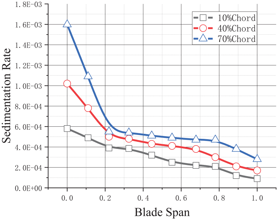
Deposition rate along with the span. A research result about the sedimentation rate on the blade surface at different chord are exhibited in Figure 2.

According to Reid’s research data, the amount of pollutants deposited on the stator blade is almost twice that on the rotor blade. In this paper, only the stator blade profile was changed to simulated the compressor performance after fouling. Figure 3 showed the different of the profile between the clean blade and fouling blade. The accumulation of contaminants will make the blades thicker after the blade has been fouled, so the fouling blade profile is thicker than the clean blade profile.

Figure 3.

Stator blade profile change. Fouling blade surface profile change compares with clean blade.

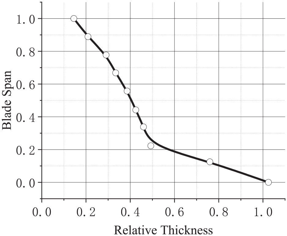
The three curves in the Figure 4 represent three different position on the chord. They have the same trend along the span, but a little different on the value. This study chooses the curve of the 40% streamline in the Figure 4 to add the thickness on the stator blade surface of the stage 35. In this study, there are six different stator blades had been set up according the different max thickness, including the clean blade. The information of the six stator blades are shown in the Table 1.

Figure 4.

Relative thickness alter against the span.

Table 1.

Scenario for simulation.

	Max thickness (μm)	Stator Ra (μm)	Rotor Ra (μm)
MT-0	0	2	1
MT-1	100	20	10
MT-2	110	20	10
MT-3	120	20	10
MT-4	130	20	10
MT-5	140	20	10

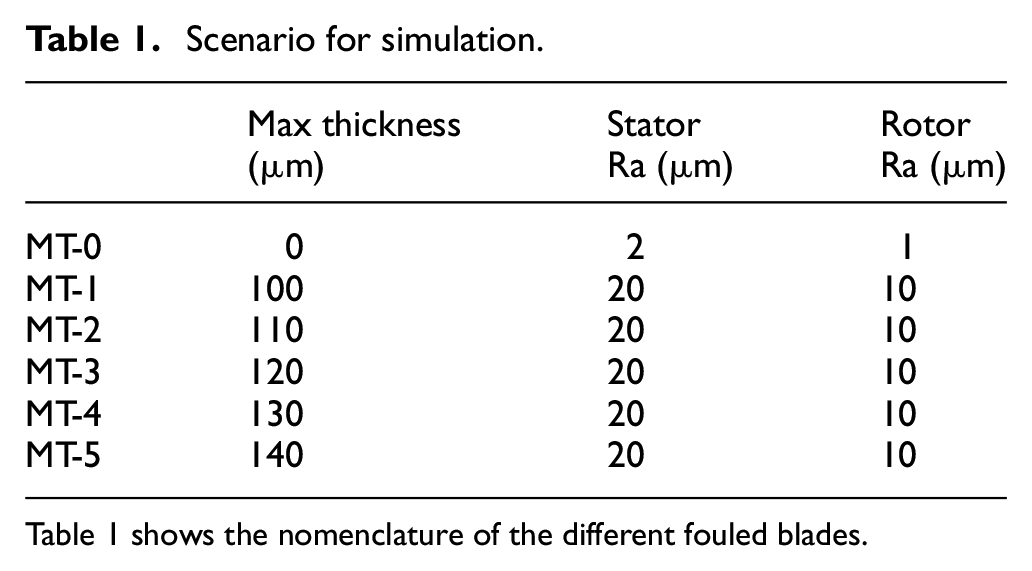
Table 1 shows the nomenclature of the different fouled blades.

Numerical simulation

ANSYSY CFX was used to simulation the effect of fouling on the stator blade. In the current study, the simulation calculation was simplified as a constant compressible viscous flow based on the working principles and pneumatic characteristics of the compressor. The blade surface will be rough after fouling. The rotor and stator blades were set as a rough wall in the simulation. The wall equation requires that the height of the first layer of the mesh should not be less than the roughness. However, if the k-omega turbulence model is used, it is necessary to ensure that the y+ is less than 1. So k-ε turbulence model was selected in the paper. The k-ε turbulence model was selected for the calculation to account for surface roughness; the near-wall model of the k-ε turbulence model must be modified with respect to the standard ones. As an index of the wall roughness, the equivalent sand-grain roughness k_s has been widely used among researchers.

For the calculation of mild fouling, the equation varies depending on the roughness of the blade surface. When the wall is set to be smooth, its function equation is:

\frac{u}{u_{t}} = \frac{1}{κ} \ln y^{+} + B_{0}

(1)

The parameters in the equation are followed:

y^{+} = \frac{y u_{τ}}{υ}

(2)

u_{τ} = \sqrt{\frac{τ_{wall}}{ρ}}

(3)

When the wall needs to be a rough wall the equation of the smooth wall should be:

\frac{u}{u_{t}} = \frac{1}{κ} \ln \frac{y - d_{0}}{k_{0}} + B_{0}

(4)

The expression of k₀ in the equation is:

k_{0} = \frac{k_{s}}{30}

(5)

In the functional equation: u is the fluid velocity; $u_{τ}$ represents the friction velocity; $τ_{wall}$ is the wall shear stress; $υ$ is the kinematic viscosity coefficient; k₀ is the equivalent surface roughness; k_s is the average surface roughness; d₀ is the base height. The $κ$ in the functional equation is the von Karman constant. Its value is 0.41, B₀ is also a constant, and its value is 5.36.¹⁷

Grid

Structured grids have the advantages of high grid quality and fast calculation speed compared to unstructured grids, so in this study the grid was generated by the structured grid generation method by ICEM CFD software. High-quality grid calculation tended to be more accurate.

In the calculation of domain grid division, a HOH-type grid structure was used. And an O-grid structure was used around the surface of the blade, the section of the blade was divided by butterfly grid structure. Cadorin et al.¹⁸ studied the effect of grid structure in roughness wall surfaces. They found that the height of the first grid should be larger than or equal to the dimensionless sand-grain roughness. If not, the calculation results will be incorrect.

The height of the first grid from the wall in this study is 30 μm and the y⁺ value of the blade surface is less than 30. When the number of grids was higher than 2.3 million, the calculation results would not change. Ultimately, the 2.3 million mesh was used, in addition, the grid was generated as illustrated in Figure 5.

Figure 5.

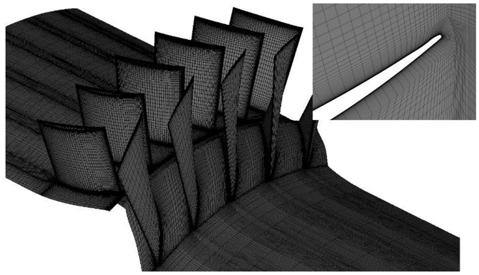
Numerical grid.

Boundary conditions

Inlet: Total pressure boundary condition was given of 101,325 Pa, and the total temperature was 288.15 K, and the air intake mode was set to axial intake.

Outlet: Static pressure outlet, control the mass flow of the compressor by change the value of the static pressure.

Wall: All wall boundary conditions were set to roughness walls. The surface roughness values of the rotor blades, shroud and hub were set to 10 μm. And 20 μm was the value of the stator blades surfaces.

Roughness before fouling: The roughness was set to 2 μm and satisfied the nonslip condition.

Model validation

Validation is performed to verify whether the established computing model and grid are accurate. The performance parameters of the model were calculated and compared with the experimental data to validate the model. Figures 6 and 7 illustrates the calculated performance characteristics of the compressor and the corresponding experimental data. The calculated results showed consistency with the experimental data; 4% was the maximum value of the error.

Figure 6.

Performance maps (total pressure ratio): comparison between experimental data and simulation results.

Figure 7.

Performance maps (isentropic efficiency): comparison between experimental data and simulation results.

Numerical results

The speed of the compressor was set to 17,188 rpm, which is the rotate speed of the NASA stage 35. Total pressure ratio and isentropic efficiency of the compressor were obtained by numerical simulation. The x-axis in Figures 8 and 9 represents the mass flow rate of the compressor, and the y-axis is the total pressure-to-pressure ratio and isentropic efficiency, respectively.

Total - to - total Pressure ratio = \frac{P_{out}^{*}}{P_{in}^{*}}

Isentropic Efficiency (η_{is}) = \frac{{(\frac{P_{out}^{*}}{P_{in}^{*}})}^{\frac{k - 1}{k}} - 1}{\frac{T_{out}^{*}}{T_{in}^{*}} - 1}

Figure 8.

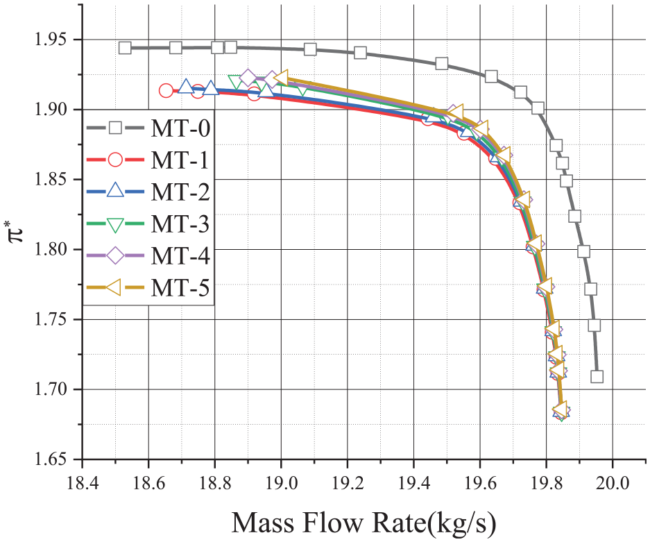
Compressor stage performance curves (total pressure ratio).

Figure 9.

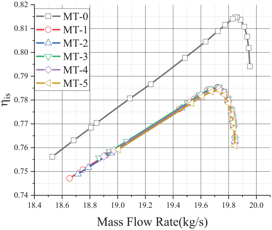
Compressor stage performance curves (isentropic efficiency).

The total pressure ratio and the isentropic efficiency values of the compressor are both deviation after increasing the thickness of the blade’s profile. Furthermore, the value of the isentropic efficiency decreases in a larger part than the total pressure ratio. The maximum degeneration of total pressure ratio and isentropic efficiency are 1.59% and 3.76%, respectively. In this paper, five different maximum thickness values were used to increase the thickness of the blade profile. However, the simulation results show that there is almost no difference in the total pressure ratio and the isentropic efficiency of the five models.

Transient calculation result was shown in Figure 10. Figure 10 was the eddy viscosity of 0.2 span at different times. Due to the change in the profile of the blade, the Eddy viscosity increases and develops further downstream of the blade. At the three timesteps, the flow field around the blade barely changed. The Eddy viscosity changed at 300% of the chord length downstream of the trailing edge of the stator blade. When the blade profile is thickened, the vortex viscosity change is eliminated.

Figure 10.

Eddy viscosity at 0.2 span.

As can be seen, fouling on the stator blade also impact the range of mass flow rate. Figure 11 shows the Area and Mach number between two stator blades. Thickness increase bring about a decrease of the channel area and an increase on the Mach number. The channel area of the MT-5 at 50% chord decreases 4.35% compare with MT-0. In addition, the Mach number increases 9.7%. Data showed that the Mach number augment make an increase of axial velocity at the outlet (downstream of the stator). The airflow angle at the exit of the stator will decrease due to this phenomenon, when the rotation speed is constant. So fouling will have a catastrophic impact on the next stage compressor.

Figure 11.

Channel area and Mach number at the 50% chord of the stator.

The mass flow rate of choke point and the stall point are plotted against the different geometry models in Figure 12. As shown in the figure, the effect of stator fouling on the mass flow rate range of compressor is negative. For every 100 μm increase in maximum thickness, the mass flow rate range decreases by 7.3%. Fouling on the stator blade only effect the stall point mass flow rate.

Figure 12.

Mass flow rate range.

For investigating the cause of the deviation in the isentropic efficiency of the compressor, it is necessary to analyze the flow field inside the compressor. A slight deviation occurs in the total pressure ratio and efficiency under the five different blade profile, only the numerical simulation results with a thickness of 100 μm are used for analysis.

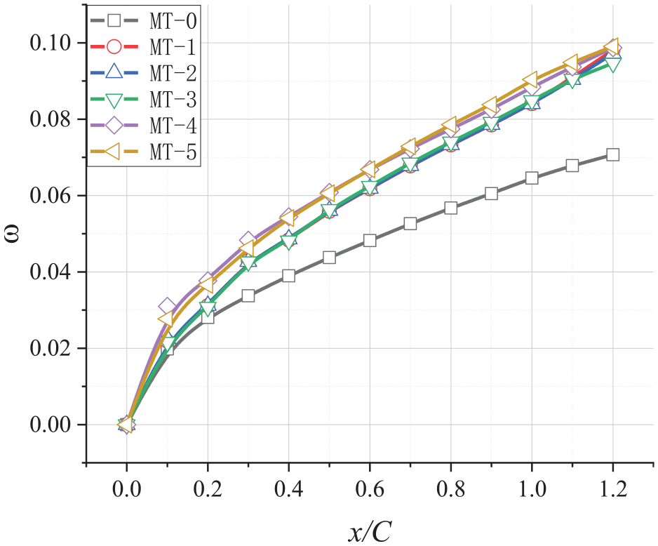
In Figure 13, total pressure loss coefficient ω is plotted against the axial position x/C.

ω = \frac{P_{t 1} - P_{tx}}{P_{t 1} - P_{1}}

(6)

Figure 13.

Total pressure loss coefficient.

Where P_t is total pressure and P is the static pressure. And the 1 represents the inlet of the stator, x is the axial position. The position x/C = 0 and x/C = 1 are the leading edge and the trail edge of the stator blade, respectively.

There is no different on the total pressure loss coefficient from leading edge to 20% chord of the six curves. The ω start to increase from 30% chord of the stator blade. The total pressure degradation cause of stator blade fouling start from 30% chord position. The total pressure coefficient increases with x/C after 20% chord, and the increase rate become larger when x/C > 1.

The isentropic Mach number along the stator blade at 20% span shown on the illustration 14. In generally, the isentropic Mach number increase after fouling on the blade surface. There is a separation bubble shown at the 30% chord of the suction side when increase the thickness. The size of the separation bubble increase with the thickness value. The fouling caused the early transition of the flow on the blade suction surface. Thickness increase barely have effect on the start position of the separation bubble. The separation bubble always start at 28% chord and disappear at 43% chord. The isentropic Mach number changed from the original trough to the crest shape at 4% chord on the pressure side. Wave crest

The pressure coefficient is defined as:

C_{p} = \frac{P - P_{1}}{P_{t 1} - P_{1}}

(7)

Where P_t₁ and P₁ refer to the upstream total and static pressure from the leading edge of stator blade, respectively. The pressure coefficient at the 20% span of the stator blade can be seen in the Figure 15.

See Figure 14 for Isentropic Mach Number on 20% Span of blade.

Figure 14.

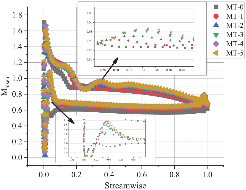
Isentropic Mach number on 20% span of blade.

Static pressure has an opposite condition at the leading edge after fouling. As shown in the Figure 15, Cp decrease a lot after fouling at the leading edge. There is no obvious total pressure loss near the leading edge after fouling, but a large drop in static pressure. More energy is reflected in the flow in the form of velocity near the leading after fouling, the phenomenon can also be found in Figure 22.

Figure 15.

Pressure coefficient on 20% Span.

The six sets of data for the clean blade surface and the fouling blade surface are shown in the figure below. There is an obvious difference that can be seen in these six curves. This curves are very different at the leading edge of the pressure surface of the blade surface. The pressure coefficient of the clean blade has an upward trend at the leading edge of the pressure surface. Conversely, the pressure coefficient of the thickened blade shows a downward trend at the leading edge of the pressure surface. Even the pressure coefficient becomes negative at the 10% chord on the pressure side.

Figure 15 shows that curves also differ near the trailing edge. Pressure coefficient attenuated compared to the clean compressor. Figure 20 shows the streamline of clean blade and fouling blade near the trailing edge at 20% span. Before the fouling, there is only a low-velocity area down the trailing edge. Fouling adds thickness on the blades, so two vortices appear down the trailing edge.

The limit streamlines has been shown in Figure 16, the vortex measurement at the trailing edge around the tip of the blade increase after fouling. The layer from the end-wall around hub and the vortex from the tip of blade squeezing the mainstream at the same time. The vortex area move to the downstream when the thickness increase, and the area decrease.

Figure 16.

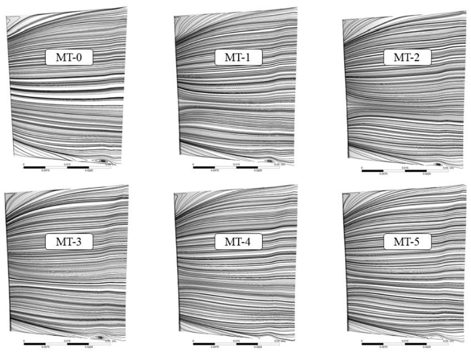
Limit streamlines on the suction side of the stator.

The vortices impact the flow field at the exit of the stator. In addition, due to the existence of vortices, a larger area of low-velocity fluid appears downstream of the trailing edge. Mixing more low-velocity fluid with high-velocity mainstream will consume more energy. The sudden increase in the total pressure loss coefficient rate downstream of the trailing edge in Figure 8 is also due to the presence of the vortices.

Static entropy of fouling blade has a significantly increase at 50% chord downstream of stator, as shown in Figures 17 and 18.

Figure 17.

Static entropy downstream of the compressor.

Figure 18.

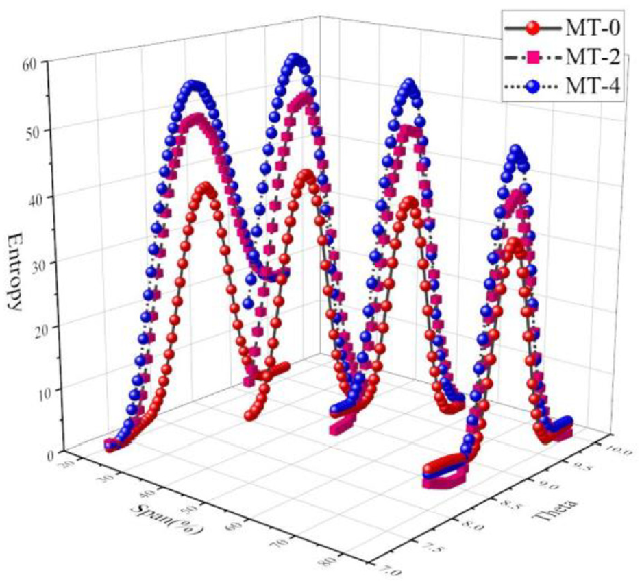
Static entropy downstream of the compressor against span.

Figure 19 shows the velocity against the blade-to-blade angle position θ_BB at 50% chord downstream the 50% span stator blade. The depth and width of the wakes increase with the fouling increase. The velocity close the suction side is larger than the pressure side. Minimum velocity of the six curves against different θ_BB. With the increase of the fouling thickness, the θ_BB corresponding to the minimum velocity is more inclined to the suction side. This conclusion is consistent with Kong’s et al.¹⁹ cascade measurement conclusion. This value in MT-5 offset 0.2° than MT-0, the turning angle of the flow after passing the stator blade was decrease. Morini⁹ also reported a similar phenomenon, which studied the effects of nonuniform roughness on the rotor blade of NASA stage 37.

Figure 19.

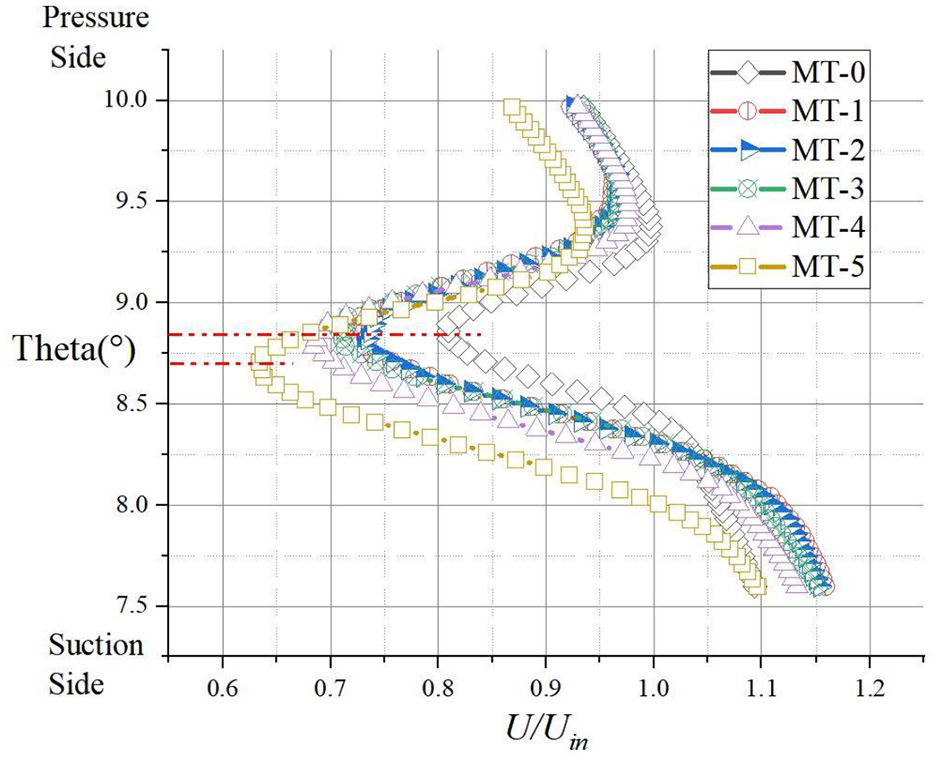
Relative velocity downstream stator.

The presence of the eddy currents in Figure 20 is the responsible for the change in the velocity along the blade-to-blade angle position after fouling. After the airflow passes through the fouling stator, the mainstream flow needs a longer distance to complete the mixing process with the low-velocity flow downstream the trailing edge. Normally, axial compressor do not exit in a single stage, and changes in the downstream flow field caused by fouling on the stator blades will effect the operation of the next stage compressor.

Figure 20.

Velocity contour and streamline of trailing edge.

The Figure 21 shows the pressure coefficient of the thickened blade. Different curves represent different span values of the blade surface. The pressure coefficient has a negative value at the leading edge of the pressure surface when the span value is less than 0.4. And this phenomenon is most obvious when the value of span is 0.1 and 0.2. The Figure 20 shows the pressure coefficient at span of 0.1. There is a low value area at the leading edge of the pressure surface.

Figure 21.

Contour of pressure coefficient at 10% span.

Observe the distribution of the Mach number at the span of 0.2 as shown in Figure 22. After the blade is thickened, the area of the high Mach number of the blade leading edge position is significantly increased. The flow area of the blade passage is reduced, and the overall flow velocity is increased slightly at the same flow rate, since the shape of the blade is thickened. At the same time, it is also noted that after the blade profile is thickened, the airflow wake at the exit of the stator blade is thickened and lengthened. In the airflow loss of the compressor, the blending loss of the wake occupies a large part, and the widening and thickening of the trail means that more blending loss will occur, which will also lead to a decrease in the efficiency of the compressor. The area of the low-pressure region near the suction surface of the blade becomes larger when the blade fouling.

Figure 22.

Channel Mach number of different span.

Conclusion

In this study, NASA Stage 35 single-stage compressor was selected as the research object, simulating the work of the compressor when the stator blade was fouled. The blade fouling was simulated by changing the blade thickness of the stator blade surface. CFX numerical code was conducted.

The performance degradation and the internal flow field of the compressor before and after fouling were compared and found that the fouling of the blade surface caused the development of the blade surface boundary layer and the low velocity airflow area became longer and longer. The impact of fouling on efficiency is more than the pressure ratio. By comparing the calculated data of different scale thicknesses, it was found that the thickness increment of the blade makes the working flow range of the compressor decrease proportionally. For every 100 μm increase in maximum thickness, the mass flow rate range decreases by 7.3%. The fouling caused the early transition of the flow on the blade suction surface. In addition the separation bubble always start at 28% chord and disappear at 43% chord. Turning angle of the flow will decrease 0.2° when the max thickness of the stator blade increases 0.15 mm.

Footnotes

Appendix

Handling Editor: James Baldwin

Declaration of conflicting interests

The author(s) declared no potential conflicts of interest with respect to the research, authorship, and/or publication of this article.

Funding

The author(s) disclosed receipt of the following financial support for the research, authorship, and/or publication of this article: The work of this paper is completed under the support of the National Science and Technology Major Project (2017-V-0002-0051); Outstanding Youth Foundation of Heilongjiang Province: YQ2019E015 and the Fundamental Research Funds for the Central Universities (3072021CF310), the author expresses its sincere gratitude to the three institutions.

ORCID iD

Li-Song Wang

References

Suman

Morini

Kurz

, et al. Estimation of the particle deposition on a transonic axial compressor blade. J Eng Gas Turbines Power 2016; 138: 012604.

Zwebek

Pilidis

Degradation effects on combined cycle power plant performance—part I: Gas turbine cycle component degradation effects. J Eng Gas Turbines Power 2003; 125: V002T04A022.

Syverud

Brekke

Bakken

LE.

Axial compressor deterioration caused by saltwater ingestion. J Turbomach 2008; 129: 119–126.

Chen

Joffre

Avitabile

Underwater dynamic response at limited points expanded to full-field strain response. J Vib Acoust 2018; 140: 051016.

Chen

Mendoza

Todd

Experimental and numerical study of high-order complex curvature mode shape and mode coupling on a three-bladed wind turbine assembly. Mech Syst Signal Process 2021; 160: 107873.

Qiao

Yang

, et al, (eds). Optimal placement of blade tip timing sensors considering multi-mode vibration using evolutionary algorithms. In: 2020 International conference on sensing, measurement & data analytics in the era of artificial intelligence (ICSMD), Xi’an, China, 15–17 October 2020, pp.367–372. New York: IEEE.

Millsaps

Baker

Patterson

, (eds). Detection and localization of fouling in a gas turbine compressor from aerothermodynamic measurements. In: ASME turbo expo 2004: power for land, sea, and air, Vienna, Austria, June 14–17, 2004, pp.1867–1876. New York: ASME.

Morini

Pinelli

Spina

, et al, (eds). CFD simulation of fouling on axial compressor stages. In: ASME turbo expo: power for land, sea, & air, Orlando, Florida, 8–12 June 2009. New York: ASME.

Morini

Pinelli

Spina

, et al. Computational fluid dynamics simulation of fouling on axial compressor stages. J Eng Gas Turbines Power 2010; 132: 331–342.

10.

Morini

Pinelli

Spina

, et al. Numerical analysis of the effects of nonuniform surface roughness on compressor stage performance. J Eng Gas Turbines Power 2011; 133: 745–753.

11.

Bons

(ed.). St and c_f augmentation for real turbine roughness with elevated freestream turbulence. In: ASME turbo expo: power for land, sea, & air, Amsterdam, The Netherlands, 3–6 June 2002. New York: ASME.

12.

Suder

KL.

Blockage development in a transonic, axial compressor rotor. J Turbomach 1998; 120: 465.

13.

Templalexis

Pachidis

Simulation of fouling in axial flow compressor using a throughflow method. J Energy Eng 2017; 143: 04016028.

14.

Reid

Moore

. Design and overall performance of four highly loaded, high speed inlet stages for an advanced high-pressure-ratio core compressor. NASA Technical Paper 1337, 1978.

15.

Moore

Reid

. Performance of single-stage axial-flow transonic compressor with rotor and stator aspect ratios of 1.63 and 1.77, respectively, and with design pressure ratio of 2.05, NASA Technical Paper, Lewis Research Center Cleveland, Ohio, 1980.

16.

Yang

H-D

. Research on the fouling mechanism and the effect of fouling on performance of axial flow compressor. Beijing, China: North China Electric Power University, 2014.

17.

Mingliang

. Research on the effects of salt spray corrosion on the compressor performance. China: Harbin Engineering University, 2013.

18.

Cadorin

Morini

Pinelli

Numerical analyses of high Reynolds number flow of high pressure fuel gas through rough pipes. Int J Hydrog Energy 2010; 35: 7568–7579.

19.

Kong

Jeong

Song

SJ.

Effects of surface roughness on evolutions of loss and deviation in a linear compressor cascade. J Mech Sci Technol 2017; 31: 5329–5335.

Simulation of the effect of nonuniform fouling thickness on an axial compressor stage performance

Abstract

Keywords

Introduction

Geometric model

Clean compressor model

Fouling compressor model

Numerical simulation

Grid

Boundary conditions

Model validation

Numerical results

Conclusion

Footnotes

Appendix

Declaration of conflicting interests

Funding

ORCID iD

References