Numerical study of the switching mechanism of a jet valve using the meshless method

Abstract

This study numerically investigates fluid dynamics of a jet flow at supersonic speed. The meshless method and the overlapping point cloud method are used to handle the moving boundary problems. The interaction between the jet flow and a moving ball-shaped plug is numerically solved, which has been rarely done in the published literature. The switching mechanism of a novel designed jet valve in an attitude and orbit control system (AOCS) is analyzed. It is found out that applied pressure to the control inlets of the jet valve must be high enough in order to successfully drive the plug to move and subsequently change the force direction acting on the jet valve. Then the switching mechanism of AOCS can be triggered. The initial fluid condition also plays a vital role and it significantly influences the response time of the switch. This study explores the underlying physics of the jet flow on its deflection, wall attachment, and interaction with the ball-shaped plug. It contributes to the optimization design of the jet valve in the AOCS with a fast and efficient response.

Introduction

Complex fluid flows with free moving solid bodies are very common engineering problems, such as multi-body interaction, free surface problems, forced vibration problems, etc. They are so-called dynamic boundary problems in computational fluid dynamics (CFD) analysis. To track the moving boundaries of the solid bodies, the commonly used numerical methodologies include mesh reconstruction method, overset mesh method, meshless method, etc. Mesh reconstruction method allows extreme deformation of the moving bodies and meanwhile controls the mesh element quality such as non-orthogonality, high skewness, and high aspect ratio. ¹ So it is robust to accurately approximate the fluid field and the body motion. But it is computationally costly. Overset mesh method uses multiple sets of meshes and remeshing is unnecessary. ² It consists of a stationary mesh for the entire background domain and moving meshes near the embedded moving bodies. Extra work is required to deal with information exchanges of mechanism interaction stored on the different sets of mesh elements during the numerical iteration. This technique has been widely employed in the CFD solver tools such as Star-CCM+, ANSYS Fluent, and OpenFOAM.

The meshless (“meshfree,”“gridless,” or “gridfree”) method only requires the information of the points created in the computational domain to solve the governing equations of fluid flow. The points are not connected into the mesh elements. This method alleviates the work of mesh generation. However, meshless method is computationally costly. ³ It was initially applied in the structural mechanics to capture large deformation of the solid bodies with relatively advanced development. ⁴ Its application in CFD can trace back to 1992. It was introduced by Batina. ⁵ Three algorithms can be used to compute partial derivatives of the fluid governing equations. They are the polynomial least-squares (PLS) method with fixed Gaussian weighting, the Taylor series least-squares (TLS) method, and radial basis functions (RBF).^6,7 The least-squares method has shown its advantages for flows with shock and can accurately predict shock locations and jumps. ⁶ Owing to the different polynomial basis functions used, the least-squares method is categorized into the least squares (LS), weighted least squares (WLS), and moving least squares (MSL). ⁷ Their relationship is summarized in Chen and Belytschko. ⁸ Oñate et al. ⁹ proposed a weight function in the least-squares method and reconstructed flux variables for spatial derivatives in order to reduce the influence of the distance between the satellite points and the center points on the solution of the fluid dynamics. It has been noted that TLS method is computationally cheapest. ⁶ TLS employs Taylor expansion formula to obtain the curve-fit equations to compute the spatial derivatives. ¹⁰ This method yields stabilization and eliminates explicitly calculating higher order derivatives. ⁸ The discretizing scheme for spatial derivatives successfully simulated the three-dimensional (3D) practical flow problems by Liu and Su. ¹⁰ Its implementation in the compressible flow has been proved to be accuracy comparable to the mesh-based finite volume method (FVM) or finite element method (FEM) and made it more competitive. ¹¹ The similar approach was developed in the reference. ¹² A global stencil of grid points was applied in the upwind method. Its order of accuracy in a 2D case and conservation of the least-squares method was evaluated to be comparative the mesh-based FVM. In present study, TLS will be used to approximate the partial derivatives in the fluid flow governing equations.

The switching mechanism of a jet valve in an attitude and orbit control system (AOCS) has wide application such as the jet hammers for drilling in the oil industry, bistable reversing valve for changing attitude of the missile in the weaponry industry, and the jet control system for the temperature control of electrolytic aluminum in the chemical industry.^13–17 The jet control idea was proposed by Joyce ¹⁸ in the 1980s. The characteristics of the main flow were changed by controlling applied pressure to the control inlets. The deflection of the jet flow triggered the switch of the flow outlet. The flow dynamics on the associated devices were consequently changed. This control method had the advantages of fast response, low cost, and high reliability. Studies on the fluid dynamics of the controlled and uncontrolled jet flow have been performed by many researchers using numerical methods. For example, Mirjalily ¹⁹ investigated the outlet flow of elliptic nozzle with the k−ω SST (shear stress transport) turbulence model. Wei et al. ²⁰ numerically analyzed the polymer additive jet flow at transonic speed using software Ansys FLUENT. The standard k−ε turbulence model was used. However, rare ones have involved moving boundary problems. The switching process of the jet valve in the AOCS will be investigated using the meshless method in this study. It is the novelty of this paper.

Many researchers performed analysis on the Jet flow about the limitation and accuracy of the used turbulence models. Kaushik et al. ²¹ reviewed the complexity of different turbulence models in resolving subsonic and supersonic jet flow inside convergent-divergent nozzles. They found that Large Eddy Simulation (LES) was more accurate than Reynolds Averaged Navier-Stokes method (RANS) and more efficient than Direction Numerical simulation (DNS). Good agreement with the experimental data was obtained in modeling turbulent jet flows at the transonic and supersonic speed. ²² Although DNS was the most accurate method, it had the limit of Reynolds number as low as 5000 in modeling complex field of the jet flow with current computer resource. ²³ Tandra et al. ²⁴ proved that the standard k−ε model of the RANS turbulence model over-predicted the growth rate of the kinetic energy of the turbulence in calculating a high-speed jet flow. So the limit of the eigenvalue of Reynolds stress and correction terms were introduced by Durbin. ²⁵ The results were improved with the modified k−ε model. When the flow separation and re-attachment occurred within the boundary layers of the solid walls, the Wilcox k−ω model showed its superior in the subsonic and transonic flow regimes. ²⁶ This turbulence model will be implemented in this study.

Numerical analysis of the switching mechanism of the jet valve using the meshless method will be performed to handle the dynamic boundary problems in this paper. The governing equations of fluid flow in the form of Arbitrary Lagrangian-Eulerian (ALE) are introduced in Section 2. The meshless method and the discretization of the mathematical derivatives in the governing equations are elaborated in Section 3. After that, the overlapping point cloud method (OPCM) is briefed to deal with the dynamic boundary problems. In Section 5, numerical methods are validated by studying the pitching oscillation of an airfoil NACA0012. The switching mechanism of the jet valve is numerical solved when pressure is applied to the different control inlets in order to deflect the main jet flow. Conclusions are drawn in the final section.

Governing equations

In the CFD analysis, there are two techniques to represent the motion of fluid: the Lagrangian method and the Eulerian method. The former defines that the fluid particles move together with the computational domain mesh. The latter considers the prior fixed domain in space and the fluid moves through the mesh elements as time passes. The Lagrangian method is vulnerable to entanglement and grid distortion in handling larger deformation. Although the Eulerian method isn’t subject to these problems, the challenge is to accurately capture the sharpness of the deformed interfaces. The concept of ALE combines both methods and takes advantage of their best features. This method is reliable to deal with the large deformation problems of solid geometries. ²⁷ In ALE technique, the compressible ideal fluid flow is governed by the Navier-Stokes (NS) equations in the differential form as,^3,28

$$\frac{\partial Q}{\partial t}+\frac{\partial E}{\partial x}+\frac{\partial F}{\partial y}+\frac{\partial G}{\partial z}=\frac{\partial E_v}{\partial x}+\frac{\partial F_v}{\partial y}+\frac{\partial G_v}{\partial z}$$

(1a)

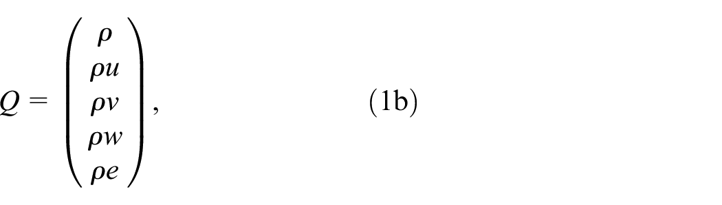
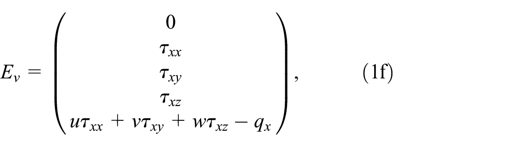
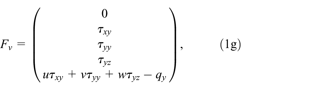
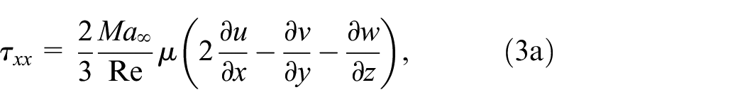
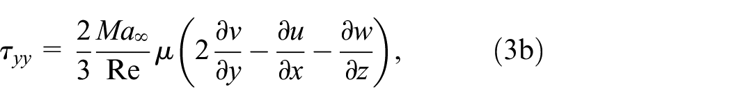
The viscous stresses are proportional to the local deformation rate. The fluid is assumed to be isotropic. For the compressible flows at transonic and supersonic speeds, the viscous regions are usually very thin and the flows in large region behave as an inviscid fluid. So the flux vectors are split into convective and viscous components.^29,30Q is the vector of conserved variables. E, F, and G are vectors of inviscid fluxes in the x-, y-, and z-direction. E_ν, F_ν, G_ν are vectors of viscous fluxes in the x-, y-, and z-direction.

$$Q=\left(\begin{array}{c}\rho \hfill \\ \multicolumn{1}{c}{\rho u}\\ \multicolumn{1}{c}{\rho v}\\ \multicolumn{1}{c}{\rho w}\\ \multicolumn{1}{c}{\rho e}\end{array}\right),$$

(1b)

$$E=\left(\begin{array}{c}\rho (u-u_t)\hfill \\ \multicolumn{1}{c}{\rho u(u-u_t)+p}\\ \multicolumn{1}{c}{\rho v(u-u_t)}\\ \multicolumn{1}{c}{\rho w(u-u_t)}\\ \multicolumn{1}{c}{\rho e(u-u_t)+\mathrm{pu}}\end{array}\right),$$

(1c)

$$F=\left(\begin{array}{c}\rho (v-v_t)\hfill \\ \multicolumn{1}{c}{\rho u(v-v_t)}\\ \multicolumn{1}{c}{\rho v(v-v_t)+p}\\ \multicolumn{1}{c}{\rho w(v-v_t)}\\ \multicolumn{1}{c}{\rho e(v-v_t)+\mathrm{pv}}\end{array}\right),$$

(1d)

$$G=\left(\begin{array}{c}\rho (w-w_t)\hfill \\ \multicolumn{1}{c}{\rho u(w-w_t)}\\ \multicolumn{1}{c}{\rho v(w-w_t)}\\ \multicolumn{1}{c}{\rho w(w-w_t)+p}\\ \multicolumn{1}{c}{\rho e(w-w_t)+\mathrm{pw}}\end{array}\right),$$

(1e)

$$E_v=\left(\begin{array}{c}0\hfill \\ \multicolumn{1}{c}{{\tau }_{\mathrm{xx}}}\\ \multicolumn{1}{c}{{\tau }_{\mathrm{xy}}}\\ \multicolumn{1}{c}{{\tau }_{\mathrm{xz}}}\\ \multicolumn{1}{c}{u{\tau }_{\mathrm{xx}}+v{\tau }_{\mathrm{xy}}+w{\tau }_{\mathrm{xz}}-q_x}\end{array}\right),$$

(1f)

$$F_v=\left(\begin{array}{c}0\hfill \\ \multicolumn{1}{c}{{\tau }_{\mathrm{xy}}}\\ \multicolumn{1}{c}{{\tau }_{\mathrm{yy}}}\\ \multicolumn{1}{c}{{\tau }_{\mathrm{yz}}}\\ \multicolumn{1}{c}{u{\tau }_{\mathrm{xy}}+v{\tau }_{\mathrm{yy}}+w{\tau }_{\mathrm{yz}}-q_y}\end{array}\right),$$

(1g)

$$G_v=\left(\begin{array}{c}0\hfill \\ \multicolumn{1}{c}{{\tau }_{\mathrm{xz}}}\\ \multicolumn{1}{c}{{\tau }_{\mathrm{yz}}}\\ \multicolumn{1}{c}{{\tau }_{\mathrm{zz}}}\\ \multicolumn{1}{c}{u{\tau }_{\mathrm{xz}}+v{\tau }_{\mathrm{yz}}+w{\tau }_{\mathrm{zz}}-q_z}\end{array}\right),$$

(1h)

where, $\rho$ , $p$ , and e represent the gas density, the pressure, and the total internal energy of the fluid per unit mass. u, v, and w are velocity components in the x-, y-, and z-direction. u_t, v_t, and w_t are the grid velocity in the x-, y-, and z-direction. q_x, q_y, and q_z are the heat fluxed alone the x-, y-, and z-direction. For an ideal gas, the pressure is given^10,30

$$p=(\gamma -1)[\rho e-\frac{\rho }{2}(u^2+v^2+w^2)],$$

(2)

$\gamma$ is the specific heat ratio which is 1.4 for the air in this study. For compressible flows, the pressure is determined by the difference between internal (thermal) energy and kinetic energy. In equations (1f), (1g), and (1h), the shear stress components are defined as ²⁸

$${\tau }_{\mathrm{xx}}=\frac{2}{3}\frac{M{a}_{\infty }}{\mathrm{Re}}\mu (2\frac{\partial u}{\partial x}-\frac{\partial v}{\partial y}-\frac{\partial w}{\partial z}),$$

(3a)

$${\tau }_{\mathrm{yy}}=\frac{2}{3}\frac{M{a}_{\infty }}{\mathrm{Re}}\mu (2\frac{\partial v}{\partial y}-\frac{\partial u}{\partial x}-\frac{\partial w}{\partial z}),$$

(3b)

$${\tau }_{\mathrm{zz}}=\frac{2}{3}\frac{M{a}_{\infty }}{\mathrm{Re}}\mu (2\frac{\partial w}{\partial z}-\frac{\partial u}{\partial x}-\frac{\partial v}{\partial y}),$$

(3c)

$${\tau }_{\mathrm{xy}}=\frac{M{a}_{\infty }}{\mathrm{Re}}\mu (\frac{\partial v}{\partial x}+\frac{\partial u}{\partial y})={\tau }_{\mathrm{yx}},$$

(4a)

$${\tau }_{\mathrm{xz}}=\frac{M{a}_{\infty }}{\mathrm{Re}}\mu (\frac{\partial w}{\partial x}+\frac{\partial u}{\partial y})={\tau }_{\mathrm{zx}},$$

(4b)

$${\tau }_{\mathrm{yz}}=\frac{M{a}_{\infty }}{\mathrm{Re}}\mu (\frac{\partial w}{\partial y}+\frac{\partial v}{\partial z})={\tau }_{\mathrm{zy}},$$

(4c)

It is noted that the rate of heat added to the fluid is due to heat conduction. So heat flux components are defined as ²⁸

$$q_x=-k\frac{M{a}_{\infty }}{\mathrm{Re}}\frac{\partial T}{\partial x}=-\frac{M{a}_{\infty }}{\mathrm{Re}}\frac{\gamma }{(\gamma -1)}(\frac{{\mu }_l}{{\mathrm{Pr}}_l}+\frac{{\mu }_t}{{\mathrm{Pr}}_t})\frac{\partial \frac{p}{\rho }}{\partial x},$$

(5a)

$$q_y=-k\frac{M{a}_{\infty }}{\mathrm{Re}}\frac{\partial T}{\partial y}=-\frac{M{a}_{\infty }}{\mathrm{Re}}\frac{\gamma }{(\gamma -1)}(\frac{{\mu }_l}{{\mathrm{Pr}}_l}+\frac{{\mu }_t}{{\mathrm{Pr}}_t})\frac{\partial \frac{p}{\rho }}{\partial y},$$

(5b)

$$q_z=-k\frac{M{a}_{\infty }}{\mathrm{Re}}\frac{\partial T}{\partial z}=-\frac{M{a}_{\infty }}{\mathrm{Re}}\frac{\gamma }{(\gamma -1)}(\frac{{\mu }_l}{{\mathrm{Pr}}_l}+\frac{{\mu }_t}{{\mathrm{Pr}}_t})\frac{\partial \frac{p}{\rho }}{\partial z},$$

(5c)

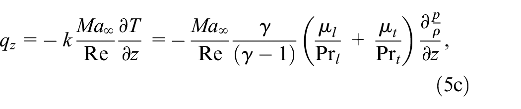
Ma_∞ is the Mach number of the incoming free stream. Re is the Reynolds number. Pr is the Prandtl number. μ is the dynamic viscosity. The subscripts l and t represent laminar flow and turbulent flow. μ _l is obtained from Sutherland’s law. μ _t value is from the selected turbulence model. In this study, Pr _l is equal to 0.72 and Pr _t is equal to 0.9. The turbulence model Wilcox $k-\omega$ is used to calculate the switching process of the jet valve of an attitude-track control engine.

Numerical methodology

The numerical algorithms of the meshless method differ from the finite difference method and the finite volume method in that the mesh topology is not required to express mathematical operators of the governing equations of fluid flow. The meshless method approximates the solution at each point of the computational domain by defining mathematical derivatives through a least squared method based on Taylor series expansions. In this study, an upwind scheme AUSM+-up is also used to compute inviscid flux terms in equation (1). The Monotonic Upstream-Centered Scheme for Conservation Laws (MUSCL) is employed to reconstruct flux variables in a Cartesian coordinate system.

Discretization of derivatives on the meshless points

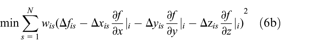
The Least Squares Method Based on Taylor Series was used to discretize the derivatives in equation (1a) on the meshless points. A cloud of point C_i is presented in Figure 1, a center point i in the computational domain is surrounded by the points s (points from 1 to N). For an arbitrary physical function $f_{\mathrm{is}}(x_{\mathrm{is}},y_{\mathrm{is}},z_{\mathrm{is}})$ , it is expanded from the center point i to the points s, ²⁷

$$\begin{array}{c}{f}_{\mathrm{is}}=f_i+(x_{\mathrm{is}}-x_i)\frac{\partial f}{\partial x}{|}_i+(y_{\mathrm{is}}-y_i)\frac{\partial f}{\partial y}{|}_i+({\mathrm{z}}_{\mathrm{is}}-z_i)\frac{\partial f}{\partial z}{|}_i\hfill \\ +O(h^2{)}_i,s=1,...,N\hfill \end{array}$$

(6a)

Figure 1.

Local point cloud C_i. The center point i and its neighboring points s from 1 to N.

For cloud C_i, the points s = 1…, N satisfy $\overline{r}\in (0,1]$ , $\overline{r}=r_i/R$ . R is the local reference radius and is equal to max ( $r_{i1},r_{i2},\dots ,r_{\mathrm{iN}}$ ), $r_{\mathrm{is}}=\sqrt{\mathrm{\Delta }{x}_{\mathrm{is}}^2+\mathrm{\Delta }{y}_{\mathrm{is}}^2+\mathrm{\Delta }{z}_{\mathrm{is}}^2}$ and $\mathrm{\Delta }{x}_{\mathrm{is}}=x_{\mathrm{is}}-x_i$ , $\mathrm{\Delta }{y}_{\mathrm{is}}=y_{\mathrm{is}}-y_i$ , $\mathrm{\Delta }{z}_{\mathrm{is}}=z_{\mathrm{is}}-z_i$ . The derivatives $\frac{\partial f}{\partial x}{|}_i$ , $\frac{\partial f}{\partial y}{|}_i$ , and $\frac{\partial f}{\partial z}{|}_i$ are obtained by applying a weighted least-square curve fit as follows,

$$min\sum _{s=1}^N{w_{\mathrm{is}}(\mathrm{\Delta }{f}_{\mathrm{is}}-\mathrm{\Delta }{x}_{\mathrm{is}}\frac{\partial f}{\partial x}{|}_i-\mathrm{\Delta }{y}_{\mathrm{is}}\frac{\partial f}{\partial y}{|}_i-\mathrm{\Delta }{\mathrm{z}}_{\mathrm{is}}\frac{\partial f}{\partial z}{|}_i)}^2$$

(6b)

where, $w_{\mathrm{is}}$ is a weight function and has the form of $w_{\mathrm{is}}=(\mathrm{\Delta }{x_{\mathrm{is}}}^2+\mathrm{\Delta }{y_{\mathrm{is}}}^2+\mathrm{\Delta }{z_{\mathrm{is}}}^2{)}^{-0.5}$

$$\mathrm{\Delta }{f}_{\mathrm{is}}=f_{\mathrm{is}}-f_i$$

(6c)

Then the derivatives in equation (1a) can be solved by the following matrix,

$$\begin{array}{c}\left[\begin{array}{ccc}\sum _{s=1}^N{w}_{\mathrm{is}}\mathrm{\Delta }{x}_{\mathrm{is}}^2\hfill & \sum _{s=1}^N{w}_{\mathrm{is}}\mathrm{\Delta }{x}_{\mathrm{is}}\mathrm{\Delta }{y}_{\mathrm{is}}\hfill & \sum _{s=1}^N{w}_{\mathrm{is}}\mathrm{\Delta }{x}_{\mathrm{is}}\mathrm{\Delta }{z}_{\mathrm{is}}\hfill \\ \multicolumn{1}{c}{\sum _{s=1}^N{w}_{\mathrm{is}}\mathrm{\Delta }{x}_{\mathrm{is}}\mathrm{\Delta }{y}_{\mathrm{is}}}& \sum _{s=1}^N{w}_{\mathrm{is}}\mathrm{\Delta }{y}_{\mathrm{is}}^2\hfill & \sum _{s=1}^N{w}_{\mathrm{is}}\mathrm{\Delta }{y}_{\mathrm{is}}\mathrm{\Delta }{z}_{\mathrm{is}}\hfill \\ \multicolumn{1}{c}{\sum _{s=1}^N{w}_{\mathrm{is}}\mathrm{\Delta }{x}_{\mathrm{is}}\mathrm{\Delta }{z}_{\mathrm{is}}}& \sum _{s=1}^N{w}_{\mathrm{is}}\mathrm{\Delta }{y}_{\mathrm{is}}\mathrm{\Delta }{z}_{\mathrm{is}}\hfill & \sum _{s=1}^N{w}_{\mathrm{is}}\mathrm{\Delta }{z}_{\mathrm{is}}^2\hfill \end{array}\right]\hfill \\ \left[\begin{array}{c}\frac{\partial f}{\partial x}{|}_i\hfill \\ \multicolumn{1}{c}{\frac{\partial f}{\partial y}{|}_i}\\ \multicolumn{1}{c}{\frac{\partial f}{\partial z}{|}_i}\end{array}\right]=\left[\begin{array}{c}\sum _{s=1}^N{w}_{\mathrm{is}}\mathrm{\Delta }{x}_{\mathrm{is}}\mathrm{\Delta }{f}_{\mathrm{is}}\hfill \\ \multicolumn{1}{c}{\sum _{s=1}^N{w}_{\mathrm{is}}\mathrm{\Delta }{y}_{\mathrm{is}}\mathrm{\Delta }{f}_{\mathrm{is}}}\\ \multicolumn{1}{c}{\sum _{s=1}^N{w}_{\mathrm{is}}\mathrm{\Delta }{z}_{\mathrm{is}}\mathrm{\Delta }{f}_{\mathrm{is}}}\end{array}\right]\hfill \end{array}$$

(7)

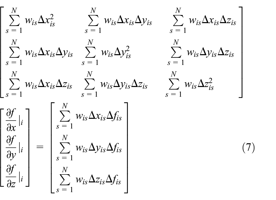
Equation (7) can be solved explicitly,

$$\frac{\partial f}{\partial x}{|}_i=\sum _{s=1}^N{\alpha }_{\mathrm{is}}\mathrm{\Delta }{f}_{\mathrm{is}},\frac{\partial f}{\partial y}{|}_i=\sum _{s=1}^N{\beta }_{\mathrm{is}}\mathrm{\Delta }{f}_{\mathrm{is}},\frac{\partial f}{\partial z}{|}_i=\sum _{s=1}^N{\gamma }_{\mathrm{is}}\mathrm{\Delta }{f}_{\mathrm{is}}$$

(8a)

The coefficients ${\alpha }_{\mathrm{is}}$ , ${\beta }_{\mathrm{is}}$ , and ${\gamma }_{\mathrm{is}}$ are,

$$\{\begin{array}{c}{\alpha }_{\mathrm{is}}=a_{\mathrm{is},1}-\frac{l_{12}}{l_{11}}{a}_{\mathrm{is},2}+\frac{l_{12}{l}_{23}-l_{13}{l}_{22}}{l_{11}{l}_{22}}{a}_{\mathrm{is},3}\hfill \\ {\beta }_{\mathrm{is}}=a_{\mathrm{is},2}-\frac{l_{23}}{l_{22}}{a}_{\mathrm{is},3}\hfill \\ {\gamma }_{\mathrm{is}}=a_{\mathrm{is},3}\hfill \end{array}$$

(8b)

where,

$$\{\begin{array}{c}{a}_{\mathrm{is},1}=\frac{\mathrm{\Delta }{x}_{\mathrm{is}}}{{l_{11}}^2}\hfill \\ \multicolumn{1}{c}{a_{\mathrm{is},2}=\frac{1}{{l_{22}}^2}(\mathrm{\Delta }{y}_{\mathrm{is}}-\frac{l_{12}}{l_{11}}\mathrm{\Delta }{x}_{\mathrm{is}})}\\ \multicolumn{1}{c}{a_{\mathrm{is},3}=\frac{1}{{l_{33}}^2}(\mathrm{\Delta }{z}_{\mathrm{is}}-\frac{l_{23}}{l_{22}}\mathrm{\Delta }{y}_{\mathrm{is}}+\frac{l_{12}{l}_{23}-l_{13}{l}_{22}}{l_{11}{l}_{22}}\mathrm{\Delta }{x}_{\mathrm{is}})}\end{array}$$

(8c)

$$\{\begin{array}{c}{l}_{11}=\sqrt{\sum _{s=1}^N{w}_{\mathrm{is}}{(\mathrm{\Delta }{x}_{\mathrm{is}})}^2},l_{12}=\frac{1}{l_{11}}\sum _{s=1}^N{w}_{\mathrm{is}}\mathrm{\Delta }{x}_{\mathrm{is}}\mathrm{\Delta }{y}_{\mathrm{is}}\hfill \\ \multicolumn{1}{c}{l_{22}=\sqrt{\sum _{s=1}^N{w}_{\mathrm{is}}{(\mathrm{\Delta }{y}_{\mathrm{is}})}^2-{l_{12}}^2},l_{13}=\frac{1}{l_{11}}\sum _{s=1}^N{w}_{\mathrm{is}}\mathrm{\Delta }{x}_{\mathrm{is}}\mathrm{\Delta }{z}_{\mathrm{is}}}\\ \multicolumn{1}{c}{l_{23}=\frac{1}{l_{22}}(\sum _{s=1}^N{w}_{\mathrm{is}}\mathrm{\Delta }{y}_{\mathrm{is}}\mathrm{\Delta }{z}_{\mathrm{is}}-\frac{l_{12}}{l_{11}}\sum _{s=1}^N{w}_{\mathrm{is}}\mathrm{\Delta }{x}_{\mathrm{is}}\mathrm{\Delta }{z}_{\mathrm{is}})}\\ \multicolumn{1}{c}{l_{33}=\sqrt{\sum _{s=1}^N{w}_{\mathrm{is}}{(\mathrm{\Delta }{z}_{\mathrm{is}})}^2-({l_{13}}^2+{l_{23}}^2)}}\end{array}$$

(8d)

The derivatives in equation (1a) can be discretized by substituting equation (8a) into it,

$$\frac{\partial Q}{\partial t}+\sum _{s\in c_i}[{\alpha }_{\mathrm{is}}(E_{\mathrm{is}}-E_i)+{\beta }_{\mathrm{is}}(G_{\mathrm{is}}-G_i)+{\gamma }_{\mathrm{is}}(F_{\mathrm{is}}-F_i)]=0$$

(9)

In the following subsections, the calculation of numerical fluxes E, F, G, E_ν, F_ν, and G_ν will be introduced.

Discretization of inviscid fluxes

According to the method proposed by Sridar and Balakrishnan, ¹² the fictitious interface J was defined at the midpoint between i and s as shown in Figure 2. In this study, the AUSM+-up scheme is used to compute the convection fluxes E_is, F_is, and G_is, and they have the following form if they are represented by f_is,

$$f_{\mathrm{is}}=\frac{1}{2}{a}_{\mathrm{is}}[m_{\mathrm{is}}({\varphi }_{\mathrm{is}}^{-}+{\varphi }_{\mathrm{is}}^{+})-\left|m_{\mathrm{is}}\right|({\varphi }_{\mathrm{is}}^{+}-{\varphi }_{\mathrm{is}}^{-})]+p_{\mathrm{is}}$$

(10a)

Figure 2.

Reconstruction of the flux f_is.

More details on this scheme can be found in the work done by Liou ³¹ and Cai et al. ³² and will not be repeated here.

The MUSCL scheme is a high order reconstruction for the flux variables. It will not cause unphysical spurious oscillations. To discretize the fluxes in the finite volume method, the basic first-order scheme upwind discretization fails to handle the larger gradients of the fluid properties and tends to smear the solution. Therefore, the MUSCL scheme together with Van Albada limiter was adopted in this study to obtain the left and right interpolated flow states and then used to calculate fluxes at the cell edges (see Figure 2). The MUSCL reconstruction scheme with a Van Albada limiter can be described as follows ³³ :

$$\{\begin{array}{c}{\varphi }_{\mathrm{is}}^{+}={\varphi }_i+\frac{S_i}{4}[(1-k{S}_i){\mathrm{\Delta }}_{\mathrm{is}}^{-}+(1+k{S}_i)({\varphi }_{\mathrm{is}}-{\varphi }_i)]\hfill \\ {\varphi }_{\mathrm{is}}^{-}={\varphi }_{\mathrm{is}}-\frac{S_{\mathrm{is}}}{4}[(1-k{S}_{\mathrm{is}}){\mathrm{\Delta }}_{\mathrm{is}}^{+}+(1+k{S}_{\mathrm{is}})({\varphi }_{\mathrm{is}}-{\varphi }_i)]\hfill \end{array}$$

(10b)

where

$${\mathrm{\Delta }}_{\mathrm{is}}^{-}=2\mathrm{\Delta }{\overrightarrow{r}}_{\mathrm{is}}•\nabla u_i-(u_{\mathrm{is}}-u_i),$$

(10c)

$${\mathrm{\Delta }}_{\mathrm{is}}^{+}=2\mathrm{\Delta }{\overrightarrow{r}}_{\mathrm{is}}•\nabla u_{\mathrm{is}}-(u_{\mathrm{is}}-u_i),$$

(10d)

where, $\mathrm{\Delta }{\overrightarrow{r}}_{\mathrm{is}}$ is the vector pointing from node $i$ to $s$ . The limiter $S$ is defined as:

$$S_i=max[0,\frac{2{\mathrm{\Delta }}_{\mathrm{is}}^{-}(u_{\mathrm{is}}-u_i)+\epsilon }{{({\mathrm{\Delta }}_{\mathrm{is}}^{-})}^2+{(u_{\mathrm{is}}-u_i)}^2+\epsilon }],$$

(10e)

$${\mathrm{S}}_{\mathrm{is}}=max[0,\frac{2{\mathrm{\Delta }}_{\mathrm{is}}^{+}(u_{\mathrm{is}}-u_i)+\epsilon }{{({\mathrm{\Delta }}_{\mathrm{is}}^{+})}^2+{(u_{\mathrm{is}}-u_i)}^2+\epsilon }],$$

(10f)

where, $\epsilon$ is a very small positive number for preventing null division and has a value of $\epsilon ={10}^{-12}$ . The parameter $k$ determines the amount of up winding and is set as $k=1/3$ .

Discretization of viscous fluxes

The gradients of the flow variables from equations (3) to (5) are calculated to discretize the viscous flux terms. The odd-even decoupling may occur if the gradient of the grid interface is calculated by averaging the values of the point i and s. Thus, a more stable numerical method of the gradient discretization was presented by May and Jameson. ³⁴ It is used in this study,

$$\nabla {\varphi }_{\mathrm{is}}=\overline{\nabla {\varphi }_{\mathrm{is}}}-(\overline{\nabla {\varphi }_{\mathrm{is}}}•{\overline{\mathrm{Sn}}}_{\mathrm{is}}-\frac{{\varphi }_{\mathrm{is}}-{\varphi }_i}{|{\overrightarrow{r}}_{\mathrm{is}}-{\overrightarrow{r}}_i|}){\overline{\mathrm{Sn}}}_{\mathrm{is}},$$

(11a)

where

$$\overline{\nabla {\varphi }_{\mathrm{is}}}=\frac{1}{2}[(\nabla {\varphi }_i)+(\nabla {\varphi }_{\mathrm{is}})],$$

(11b)

$${\overline{\mathrm{Sn}}}_{\mathrm{is}}=({\overrightarrow{r}}_{\mathrm{is}}-{\overrightarrow{r}}_i)/|{\overrightarrow{r}}_{\mathrm{is}}-{\overrightarrow{r}}_i|,$$

(11c)

Temporal discretization

The explicit three-stage Strong Stability Preserving (SSP) Runge-Kutta method is employed to advance the time evolution. The semi-discrete form of the NS equations can be written as follows ³⁵ :

$$\frac{\partial Q_i}{\partial t}+R_i=0,$$

(12a)

The solution is advanced to $Q_i^{n+1}$ over a time step $\mathrm{\Delta }t$ at time $t^{n+1}$ by:

$$Q_i^{(1)}=Q_i^n-\mathrm{\Delta }t{R}_i(Q_i^n),$$

(12b)

$$Q_i^{(2)}=\frac{3}{4}{Q}_i^n+\frac{1}{4}[Q_i^{(1)}-\mathrm{\Delta }t{R}_i(Q_i^{(1)})],$$

(12c)

$$Q_i^{n+1}=\frac{1}{3}{Q}_i^n+\frac{2}{3}[Q_i^{(2)}-\mathrm{\Delta }t{R}_i(Q_i^{(2)})],$$

(12d)

The local time step and the implicit residual smoothing technology are used to reach fast convergence.

Overlapping point cloud method

In the meshless method, sets of discrete points are distributed around the moving solid bodies. They are relatively stationary and store the characteristic information of local fluid flow. ³⁶ Set of background discrete points is generated and remains fixed while the solid bodies are moving. Their topology doesn’t change during the numerical iteration. For the overlap regions, a special meshless “point cloud” is used to perform fluid information exchange among multiple sets of the discrete points. The technique described here is known as OPCM. Compared with overset mesh method or mesh reconstruction method, the OPCM does not require to consider the restrictions of the dynamic mesh or deformation limit. The moving boundary problems can be easily solved as only discrete points are required.

Results and discussion

Pitching oscillation of a NACA0012 airfoil

The OPCM was used to solve a moving boundary problem, pitching oscillation of a NACA0012 airfoil. A set of discrete points was generated around the airfoil and would move together with the airfoil. Another set of discrete points was generated in the entire domain and remained stationary during the calculation. The distribution of two sets of points in the computing domain is shown in Figure 3 with different colors. The green ones are stationary background points and the red ones are moving points surrounding the airfoil. The angle of attack α of the NACA0012 airfoil can be expressed by the sinusoidal function during the pitching oscillation, ³⁷

$$\alpha (t)={\alpha }_0+{\alpha }_m\sin (2\kappa t),$$

(13)

where, ${\alpha }_0$ is the initial angle of attack, ${\alpha }_m$ is the amplitude of the pitch, $\kappa$ is the reduced frequency of a dimensionless number, $\kappa =\omega c/2u_{\infty }$ , where ω is angular frequency, c is the chord length of the airfoil, and u_∞ is incoming flow speed. The experimental results of the AGARD NACA0012 CT2 and CT5 by Landon are used for benchmarking on the present numerical methods. ³⁷

Figure 3.

The distribution of discrete point clouds in the computing domain: (a) α = 0° and (b) α = 7.75°.

Figures 4 and 5 show the comparison between numerical and experimental results of CT2 and CT5 on the lift coefficient C_L and the pitching-moment coefficient C_M. Their consistency proved the reliability of the OPCM in solving the dynamic boundary problem. The same numerical method was used to calculate the shifting process of a ball-shaped plug within a jet valve of the AOCS in the following context.

Figure 4.

Comparison between numerical and experimental results of CT2 on the lift coefficient C_L and the pitching-moment coefficient C_M of the NACA0012 airfoil: (a) lift coefficient C_L and (b) pitching-moment coefficient C_M.

Figure 5.

Comparison between numerical and experimental results of CT5 on the lift coefficient C_L and the pitching-moment coefficient C_M of the NACA0012 airfoil: (a) lift coefficient C_L and (b) pitching-moment coefficient C_M.

Switching mechanism of a jet valve in the AOCS

Figure 6 shows the schematic view of a fluidic bistable amplifier/switch. ³⁸ A Laval nozzle consists of one supply inlet ①, two control inlets ② at the nozzle throat, and two outlets ③. A splitter ④ is at the bottom to separate the flow. Two vents ⑤ are at each side. b is the width of the nozzle throat, d is the thickness, and 2φ is the expansion angle. The high-speed flow enters the supply inlet and accelerates in the narrow throat and forms a jet flow in the diverging chamber. Then it symmetrically passes through the nozzle ideally and exits from the two outlets if both control inlets are firmly closed. Vortices may be formed on both sidewalls of the diverging chamber. Any disturbance such as vortices in the flow can cause the jet flow to deflect to one sidewall and consequently form the wall attachment on that sidewall. The control inlets are purposely used to introduce the disturbing flow. For instance, as shown in Figure 6, a flow is introduced through the left control inlet. The jet flow below the control inlets is forced to shift right. Wall attachment on the right sidewall is formed. Vortices present on the opposite sidewall.

Figure 6.

A fluidic bistable amplifier/switch. ³⁸

The configuration of the fluidic bistable amplifier/switch in Figure 6 is applied to the engine jet valve in the AOCS. Its 3D schematic and cross-sectional views are displayed in Figure 7. A free-moving solid ball acts as a plug positioned below the splitter. The vents are two big cylindrical pipes at the bottom. In this study, four cases were analyzed as listed in Table 1. In case 1, both control inlets were closed and their entries were treated as the solid wall. The pressure P = 10.0 MPa was applied to the supply inlet. After the flow field was stabilized in the simulation, the contour of velocity magnitude was plotted in Figure 8(a). The flow from the control inlet accelerated to be supersonic in the throat and formed a jet flow in the diverging chamber. Wall attachment is visible on the right sidewall in Figure 8(b). The vortices are formed on the opposite side. The jet flow exits the right vent by the right-top corner. The left vent was completely closed by the ball-shaped plug. This is different on the design as indicated in Figure 6 where both vents are open and one for jet flow outlet. In this case, the pressure P was 4.35 MPa at both control inlets after the flow stabilized.

Figure 7.

Model of the jet valve used in AOCS: (a) 3D schematic view and (b) cross-sectional view.

Table 1.

Numerical study cases and controls to the control inlets.

Case no.	Left control inlet	Right control inlet
1	Closed	Closed
2	Closed	Open (P = 5 MPa)
3	Closed	Open (P = 6 MPa)
4	Open (P = 6 MPa)	Closed

Figure 8.

(a) Contour of velocity magnitude (m/s) and (b) flow streamline of case 1.

To force the ball-shaped plug move left and close the left vent, the right control inlet needs to be opened to introduce the side flow to interfere with the main jet flow. Ideally, the jet flow will deflect in the throat of the nozzle and shift to the left sidewall in the diverging chamber. The pressure increases on the right side. Then the jet flow shifts left even further. At last, it quickly attaches to the left sidewall. The wall attachment causes the pressure to increase on the left side of the ball-shaped plug. Consequently, the ball-shaped plug is forced to move right to close the entry of that side vent. The flow outlet is thus exchanged. The force acting on the jet valve is switched to the opposite direction. In this manner, the moving direction of the engine jet valve is controlled efficiently by applying pressure to the control inlets.

In case 2, pressure inlet boundary condition was instead applied to the right control inlet with pressure P = 5 MPa. The converged numerical results of case 1 were set as the initial flow condition in this case. Contours of instantaneous velocity magnitude are presented in Figure 9. The jet flow had the highest speed in the throat of the nozzle because of the high pressure of 10 MPa applied to the supply inlet at t = 0 ms. It started to deflect at the top of the diverging chamber after the disturbing flow was introduced from the right control inlet at t = 3.0 ms (Figure 9(b)). The pressure gradually increased near the right sidewall. Consequently, the flow deflection grew into a round bracket shape at t = 9 ms as shown in Figure 9(c). The jet flow reached stability at t = 25 ms and exited the nozzle by the right vent (Figure 9(e)). However, the ball-shaped plug stood still. This meant that the applied pressure of 5 MPa to the right control inlet was not high enough to overcome the static inertia of the ball-shaped plug. The switching mechanism of AOCS was not triggered.

Figure 9.

Contours of the instantaneous velocity magnitude (m/s) when pressure P = 5.0 MPa was applied to the right control inlet in case 2: (a) t = 0.0 ms, (b) t = 3.0 ms, (c) t = 9.0 ms, (d) t = 15.0 ms, and (e) t = 25.0 ms.

In case 3, the higher pressure of 6MPa was applied to the right control inlet. The left control inlet was still closed. The converged results of case 1 were also used as the initial condition. The aim was to find out if the higher pressure applied to the right control inlet could drive the ball-shaped plug to move and switch the jet valve. The numerical results of contours of the instantaneous velocity magnitude are presented in Figure 10. In the same way as case 2, the jet flow deflected left at the top of the diverging chamber of the nozzle because of the increased pressure on the right side. The pressure on the left sidewall was lower than on the opposite sidewall. The jet flow was forced to shift closer to the lower pressure sidewall. It finally attached itself to the left sidewall. A round bracket-shaped jet flow was visible at t = 6 ms (Figure 10(b)) and it touched the splitter at t = 10 ms (Figure 10(c)). At t = 11.96 ms, the jet flow was separated by the splitter to the left and right sides of the ball-shaped plug (Figure 10(d)). This caused the pressure to increase on the left side of the ball-shaped plug until the static inertia of the plug was overcome. The plug moved right. The jet flow squeezed into the left vent and accumulated into a fan-shaped zone at t = 13.2 ms as presented in Figure 10(e). The complete wall attachment on the left sidewall caused the pressure to increase on the left side of the ball-shaped plug. At t = 14.5 ms as shown in Figure 10(f), the ball-shaped plug was driven to move right further. More flow exited the nozzle by the left vent. The pressure was lower on the right side of the ball-shaped plug than on the opposite side. The ball-shaped plug moved right further until finally closed the right vent as presented in Figure 10(g). The flow exited the nozzle only by the left vent. The whole shift process of the ball-shaped plug from left to right took about 20.0 ms before the flow was stable. The stable pressure was about 5.97 and 4.95 MPa at both right and left control inlets. In this manner, the switching mechanism of the jet valve was successfully achieved and the position of AOCS could be controlled.

Figure 10.

Contours of the instantaneous velocity magnitude (m/s) when pressure P = 6.0 MPa was applied to the right control inlet in case 3: (a) t = 0.0 ms, (b) t = 6.0 ms, (c) t = 10.0 ms, (d) t = 11.96 ms, (e) t = 13.2 ms, (f) t = 14.5 ms, and (g) t = 20.0 ms.

Figure 11 shows the pressure variations against time on the center points of both outlets of the vents. The pressure remained nearly constant when the deflection of the jet flow occurred at the top of the diverging chamber of the nozzle before 5 ms. The pressure on the right outlet was higher during 5–12 ms because of the introduced flow from the right control inlet. It decreased from 12 to 18 ms after the jet flow was separated by the splitter and the ball-shaped plug was forced to shift from left to right as shown in Figure 10(d) and (e). After the complete wall attachment formed on the left sidewall from 18 ms onwards and the plug moved further right, the pressure in the left vent outlet increased as shown in Figure 11. This increase ceased after the right vent was completed closed by the ball-shaped plug. The stable pressure occurred at about 20.0 ms for both vents.

Figure 11.

Pressure history at the outlets of vents for case 3.

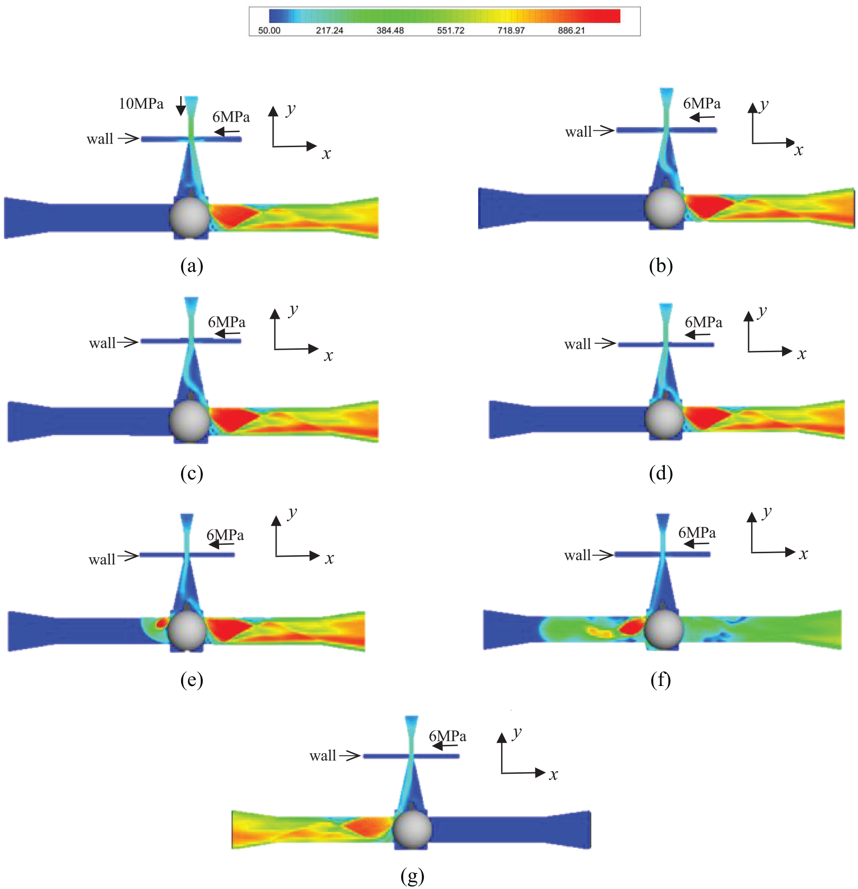
In case 4, the right control inlet was closed and the left one was opened instead. Pressure inlet boundary condition was applied to the left control inlet with P = 6 MPa. The converged results of case 3 were set as the initial flow condition. The flow field as shown in Figure 10(g) was the start moment t = 0 ms for case 4 (Figure 12(a)). The numerical results of contours of the instantaneous velocity magnitude are presented in Figure 12. A round bracket-shaped jet flow was visible because of its deflection inside the diverging chamber as shown in Figure 12(b). The jet flow displayed the same fluid dynamics as case 3, except for the delay for the jet flow to be separated by the splitter. It occurred at t = 17.1 ms while it was at t = 11.96 ms for case 3. The flow velocity in the left vent was still very high during the ball shifting period between 18.36 and 19.3 ms. The longer time was taken for the ball-shaped plug to close the right vent. Complete wall attachment on the right diverging wall was formed at t = 23.5 ms. Flow stability was achieved at 25 ms as presented in Figure 12(g) and the flow exited the nozzle only by the left vent. The whole switching processing for case 4 took 5 ms longer than case 3.

Figure 12.

Contours of the instantaneous velocity magnitude (m/s) when pressure P = 6.0 MPa was applied to the left control inlet in case 4: (a) t = 0.0 ms, (b) t = 7.0 ms, (c) t = 17.1 ms, (d) t = 18.36 ms, (e) t = 19.3 ms, (f) t = 23.5 ms, and (g) t = 25.0 ms.

Figure 13 shows the pressure variations against time on the center points of both outlets of the vents in case 4. The trend is nearly the same as in Figure 11. But the ball-shaped plug takes 5 ms longer time than case 3 to accomplish one round shift from one side to the opposite side. Moreover, the pressure in the right outlet of the vent is not constant before it starts to increase at about 18 ms. This is different from case 3 where the pressure remains the same before 15 ms as shown in Figure 11.

Figure 13.

Pressure history at the outlets of the vents for case 4.

Force variations on the ball-shaped plug are presented in Figure 14. The red curve is for case 3 and the blue curve is for case 4. Positive force is from left to right. For both cases, a reduction in force magnitude took place when the round bracket-shaped jet flow nearly touched the splitter. The direction of force acting on the ball-shaped plug started to change when the jet flow was separated by the splitter. These moments were indicated with the dashed lines in Figure 14. To accomplish a shifting process for the ball-shaped plug from one side to the opposite side, it took about 20 ms in case 4 and about 17 ms in case 3. The longer time was wasted to deflect the jet flow in the beginning in case 4. That is, the control to the jet valve in ACOS was slowed. The difference is due to the applied initial flow condition to the control inlets. For both cases, the directions of the forces acting on the ball-shaped plug were successfully changed. It indicated that the switching process of the jet valve in the AOCS was successfully achieved.

Figure 14.

Force acting on the ball-shaped plug during shifting process from one side to the opposite side for case 3 and 4.

Conclusions

In this study, the governing equations of fluid flow in the form of ALE was numerically solved to approximate a moving solid body in supersonic flow. The meshless method and the overlapping point cloud method were employed to capture the dynamic solid boundaries. A high order reconstruction technique was introduced to recover the clouds of the meshless points to be homogeneous whenever their distributions were highly anisotropic within the viscous boundary layer of the solid wall. In this manner, the accuracy of the numerical solutions on the moving boundary problems was greatly improved. The numerical methodology has been validated to be reliable in studying pitching oscillation of an airfoil.

The complex fluid dynamics of a compressible jet flow at the supersonic speed were numerically modeled to study the switching mechanism of a jet valve in an AOCS. The characteristics of the jet flow in the diverging chamber of the nozzle were clearly captured. Wall attachment of the jet flow on one sidewall was changed to the other side by introducing the disturbing flow from the control inlets. It caused the ball-shaped plug to move to the opposite side and subsequently close that side vent. The flow had to exit the nozzle by the other vent. Thus, the direction of the force acting on the jet valve was successfully changed. In this manner, the switching mechanism of the engine jet valve in the AOCS was successfully completed. The underlying fluid dynamics were analyzed. It was found out that the applied pressure in the control inlet had to be high enough to overcome the static inertia of the ball-shaped plug firstly. For the present jet valve design, the ball-shaped valve failed to move if the applied pressure to the control inlet was lower than 5.0 MPa while the applied pressure to the supply inlet was fixed at 10.0 MPa. The operation of open/close the vents was smoothly completed when the applied pressure was increased to 6.0 MPa from 5 MPa. The initial flow state was another critical factor. It influenced the response time taken by the jet valve to switch the force direction. This study contributes to the optimization design of the jet valve in the AOCS with a fast and efficient response. It also provides a clue to understand the physics of the interaction between the jet flow and the moving solid body.