
Abstract
Accurate estimation of the degree of battery aging is essential to ensure safe operation of electric vehicles. In this paper, using real-world vehicles and their operational data, a battery aging estimation method is proposed based on a dual-polarization equivalent circuit (DPEC) model and multiple data-driven models. The DPEC model and the forgetting factor recursive least-squares method are used to determine the battery system’s ohmic internal resistance, with outliers being filtered using boxplots. Furthermore, eight common data-driven models are used to describe the relationship between battery degradation and the factors influencing this degradation, and these models are analyzed and compared in terms of both estimation accuracy and computational requirements. The results show that the gradient descent tree regression, XGBoost regression, and light GBM regression models are more accurate than the other methods, with root mean square errors of less than 6.9 mΩ. The AdaBoost and random forest regression models are regarded as alternative groups because of their relative instability. The linear regression, support vector machine regression, and k-nearest neighbor regression models are not recommended because of poor accuracy or excessively high computational requirements. This work can serve as a reference for subsequent battery degradation studies based on real-time operational data.
Keywords
Introduction
With the continuing development of the social economy, both environmental pollution and the energy crisis are increasing, and the need to develop new energy vehicles such as electric vehicles (EVs) has become a general consensus worldwide.1, 2 Lithium-ion batteries have gradually become the main energy storage system for EVs because of their high energy density, long service life and high operating voltages.3, 4 However, because of a variety of side reactions, lithium-ion batteries inevitably suffer performance degradation during practical application.5, 6 It is generally believed that when the internal resistance of a lithium-ion battery increases by 100% or its capacity declines to 80% of the original capacity, it will no longer be suitable for continued use in new energy vehicles and must be replaced in a timely manner. 7 On the one hand, lithium-ion battery performance deterioration leads to poor vehicle dynamics, a reduced driving range and increased safety hazards; on the other hand, the state of health (SOH) of a lithium-ion battery cannot be measured using parameters that are measured directly by sensors. Therefore, it is important to estimate the lithium-ion battery SOH accurately based on easily collected parameters such as the battery voltage and temperature for application and promotion of EVs. 8
A wide variety of battery SOH estimation methods have been proposed in the literature and can generally be classified as direct measurement methods, indirect analysis methods, model-based methods and data-driven methods. 9 Direct measurement methods have very high measurement environment and equipment requirements, are almost impossible to apply under realistic vehicle conditions and are usually used for calibration and result accuracy check control applications. 10 Indirect analysis methods obtain information such as the battery SOH indirectly by analyzing collected battery degradation data. For example, Zheng et al. transformed the charging voltage curve using a combination of incremental capacity analysis (ICA) and differential voltage analysis (DVA) to provide a more intuitive approach to extraction of the health factors that reflect the degree of battery aging.11, 12 Li constructed the incremental capacity curve using larger multiplier currents, which reduced the accuracy of the analysis but improved the applicability of the method to practical applications. 13 Although this type of method can obtain rich information content with high accuracy, it generally relies on use of laboratory-specific equipment and the basis of a more ideal environment, and its accuracy is difficult to guarantee in practical applications because of sensor accuracy limitations and the variability of the environment. Model-based methods usually involve the construction of electrochemical models or equivalent circuit models for parameter identification to reflect the battery SOH. Electrochemical models use nonlinear coupled partial differential equations to describe the battery mechanism, which can reflect the electrochemical reaction mechanism occurring inside the battery monomer, 14 but these models are difficult to solve and require intensive computation to achieve rapid online estimation of the battery SOH. 15 The equivalent circuit model (ECM) uses basic components such as resistors, inductors and capacitors to form a circuit model to simulate the static and dynamic behavior of the battery. 16 Using the constructed battery model, the battery characterization parameters are identified using least squares, 17 extended Kalman filtering 16 and particle filtering 18 methods to obtain the battery SOH. The main drawbacks of this method are its lack of physical meaning and the inaccurate solutions obtained under some conditions. 19 In recent years, there have been increasing numbers of studies related to battery health state estimation based on data-driven methods, e.g. support vector machines, 20 XGboost, 21 radial basis function neural networks 22 and long- and short-term memory networks.23, 24 Data-driven approaches do not need to focus on the battery operating mechanism and model; instead, they focus more on the relationship between the input excitation and the target response, meaning that the application effect is solely dependent on the collected battery aging data.
However, the datasets used in most current studies are often collected under close to ideal conditions in the laboratory and thus ignore some conditions that may have unknown effects during actual vehicle operation; this may lead to poorer results being obtained from the constructed SOH models in practical applications. In addition, the test objects are often battery cells, while the batteries are always used in groups with specific series-parallel connections in practical applications, and this inconsistency may also affect practical application of the SOH estimation models developed on the basis of laboratory results. 25
To solve the problems described above, this paper proposes a battery SOH estimation model based on a large quantity of battery data collected from real EVs. The main contributions of this study are represented by the following three aspects. First, a large amount of real data collected from vehicles during actual operation is used as the basis for the model, thus better reflecting the real working state of the power battery system when compared with the laboratory test data. Second, a variety of machine learning models for power battery SOH estimation are compared in terms of both their accuracy and the computational effort required. Finally, the effectiveness of the battery SOH estimation method is verified using other vehicle datasets that differ from the training set data.
Section II of this paper describes the data acquisition and preprocessing procedure used for battery SOH estimation. Section III presents the dual-polarization equivalent circuit (DPEC) model and the parameter identification process used to obtain the ohmic internal resistance (OIR). Section IV compares the OIR estimation effectiveness performances of various machine learning models, and Section V summarizes the main conclusions. Figure 1 shows a framework diagram of the battery OIR estimation scheme.
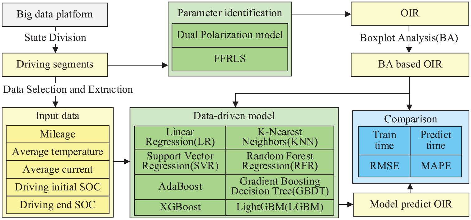
Framework diagram of battery ohmic internal resistance (OIR) estimation scheme
Data Acquisition and Processing
The data set used in this study comes from the National Monitoring and Management Center for New Energy Vehicles (NMMC-NEV) platform located in China. Data from this platform are uploaded in real-time from new energy vehicles operating in various provinces and cities in China; the recorded data include the speed and accumulated mileage of the vehicle, along with the voltage, current, state of charge (SOC), maximum temperature and minimum temperature of the battery system, which are recorded at a sampling interval of 10 s. The data format is shown in Table 1. In addition, the most important vehicle components can also be obtained from this platform. The battery system of the vehicle studied in this paper consists of 91 series-connected LiNixCoyMnzO2 (NCM) battery cells with a rated energy of 30.4 kWh and a rated voltage of 332 V; the details of the system are given in Table 2. Six electric passenger vehicles operating in Beijing were selected for the study in this paper, and the data cover the period from May 2017 to March 2019 with mileages ranging from approximately 80,000 km to 280,000 km.
Samples of time-series data collected from the NMMC-NEV data platform

Specifications of the vehicle model under study

The data sets are collected from real running EVs and are transmitted to the platform via wireless communication. Therefore, during the data collection, storage, and transmission stages, data distortion and data loss are inevitable. Therefore, some pre-processing of the data is required. First, any missing data are filled by interpolation and corrected for outliers, and the continuous data set is then divided into two parts: charging and driving. This paper focuses on OIR estimation based on the driving segment. Figure 2 shows the data acquired from a driving segment for the vehicle under study.

Speed, mileage, temperature, voltage, current, and SOC acquired during driving for the vehicle under study
Modeling and parameter identification
The purpose of this section is to establish the ECM, identify the model parameters, and obtain the OIR of the actual vehicle battery system to construct the subsequent data-driven model and thus explore the change in the OIR with the decline in the battery’s health.
Equivalent circuit model construction
Because of the capacity and power limitations of lithium-ion battery cells, EV power batteries are generally composed of multiple battery cells connected in series and parallel and are applied to vehicle power battery systems in the form of battery packs. Two methods can be used to model the equivalent circuit of EV power batteries. The first method is to model the battery cell as an object and then connect the battery system in series and parallel in accordance with the actual battery system connections to complete the ECM; however, this approach has the disadvantage of the contact resistance at the series-parallel connections within the battery pack being difficult to consider. The second method is to build the ECM by treating the power battery system as a whole 26 and, on the basis of describing the dynamic characteristics of the battery, to take the influence of the internal resistance of the external battery contact fully into consideration. In this paper, the second approach is used. In addition, based on the consideration that the actual battery series and parallel connection methods are often different for different battery models, modeling of the battery system as a whole helps to expand the applicability of the method proposed in this paper.
The Rint model, the Thevenin model and the DPEC model are the most commonly used ECMs, 27 and use of larger numbers of resistor-capacitor (RC) circuits in series enables the model to simulate the battery behavior more realistically, but this will also lead to difficulties in identifying the model parameters. In practical applications, the specific model that is used is often determined based on a combination of accuracy and complexity requirements. Because the purpose of construction of the ECM in this study is to provide labels for the training data for the subsequent machine learning model and the data platform also has strong computational capabilities, the DPEC model is selected for use in this study. The DPEC model structure is shown in Figure 3 and consists of an ideal voltage source, a series resistor, and two RC circuits. In this model, Ut represents the battery pack terminal voltage, I represents the total circuit current, Uoc represents the open circuit voltage, and R0 represents the ohmic resistance of the battery. The RD1, CD1 parallel circuit is used to characterize the electrochemical polarization effect that occurs during the charging and discharging processes of the battery, which is produced over a short time period; in addition, the RD2, CD2 parallel circuit is used to characterize the concentration difference that occurs during the charging and discharging process of the battery, which has a longer time scale.

Schematic of the DPEC battery model
According to Kirchhoff’s law, the system state-space equations can be expressed as follows:


Practical applications require discretization, and a detailed derivation of the n-RC model has been presented in the literature. 28 In this paper, we present the results directly using

where the data matrix

Parameter identification
The forgetting factor recursive least squares (FFRLS) method is used to identify the model parameters online and combines the advantages of a strong adaptive ability with a requirement for a small number of calculations. The following equation system gives the method used for online identification of model parameters by the FFRLS method. 29
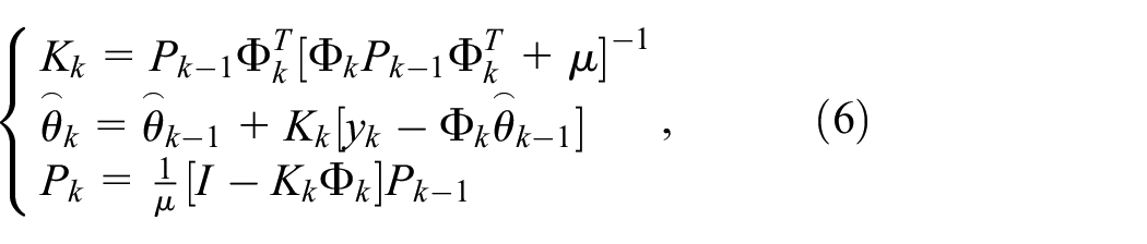
where
The OIR identification process for a single driving segment is shown in Figure 4(a) and it can be seen from the figure that the OIR converges and stabilizes rapidly when the data are input. The results for the actual terminal voltage and the model parameter identification terminal voltage are shown in Figure 4(b). The figure shows that the terminal voltage calculated by the parameter identification process is very close to the actual terminal voltage and the maximum error does not exceed 0.6 V, which indicates that the DPEC model and the FFRLS-based identification method can simulate the EV battery system characteristics very well.

Schematic diagrams of parameter identification results: (a) OIR; and (b) end voltage
Figure 5(a) shows the relationship between the OIR and the temperature, which is basically in accordance with the relationship from the Arrhenius model. Because of the existence of data distortion within the actual data acquisition, storage, and transmission process, the OIR obtained from the parameter identification approach inevitably deviates from the actual level. Because temperature is one factor that influences the OIR most strongly 21 and the temperature remains relatively stable during driving of the actual car, we screen the OIR here several times under the same temperature condition based on the boxplot; finally, we obtain the OIR data for the normal mileage under all temperatures and then fit the screened data. The fitting effect is illustrated in Figure 5(b).

Schematic diagrams of OIR versus temperature: (a) not screened; and (b) after boxplot screening
Figure 6 shows the variations of the screened OIR with the accumulated vehicle mileage for two vehicles. The OIR increases in tandem with the accumulated vehicle mileage for operation at the same temperature, which is consistent with the conclusion that the OIR increases with increasing charge/discharge times taken from traditional studies. The rate of this increase in the OIR varies for different temperatures, with lower temperatures leading to greater rates of increase in the OIR, which also matches the results of previous laboratory studies. 30 In addition, the variation of the OIR with the cumulative vehicle mileage for the different vehicles shows a similar pattern, but the slope of the curve differs for the different vehicles. This is related to the daily use behavior of each vehicle, the maintenance strategies used, or other unknown factors.
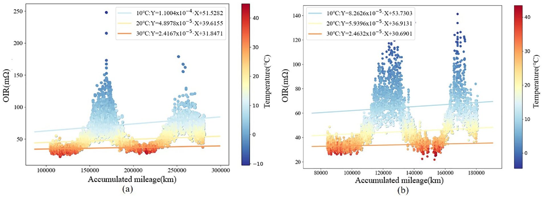
Schematic diagrams of relationship between OIR and accumulated mileage for two vehicles
Battery OIR estimation model
Studies that use machine learning algorithms for battery SOH estimation based on data sets collected from laboratory measurements have become increasingly common. These studies usually require setting of several well-controlled conditions, including a constant ambient temperature and the typical operating loads, to perform accelerated aging tests on batteries and thus collect the required battery parameters. However, laboratory-based aging tests do not reflect the realistic operating scenarios of EVs fully, which may lead to a lack of accuracy for the SOH estimation models developed based on this laboratory data. A feasible way to overcome this problem is to develop a battery SOH estimation model based on data that are collected during actual operation of the vehicle.
The power battery SOH estimation problem is a regression problem. Several classical models have been used to solve regression problems, including linear regression, k-nearest neighbor (KNN) regression, 31 and support vector machine regression. 20 In addition, neural network models have been applied increasingly widely in recent years, with fuzzy neural network (FNN),32, 33 long short-term memory (LSTM), 3 and gated recurrent unit (GRU) 34 approaches being used to solve regression problems. The principles of these different regression models are quite different and therefore have different application scenarios. Selection of the appropriate regression model for a specific problem can often achieve twice the results while requiring only half the effort. In this section, several common regression models are applied to training based on real vehicle operation data; a number of other vehicles with different data from those in the training set are then used for model validation, and the effects of these regression models are compared in terms of both their accuracy and the computational effort required.
Analysis of influencing factors
Before the OIR estimation model is built, it is necessary to analyze the factors that affect the oir to determine the required inputs for the model. Large numbers of studies have shown that battery. aging can be influenced by a variety of factors. In the power battery aging studies based on laboratory measurement data in the literature, the number of cycles, the system temperature, the charge/discharge multiplier, and the depth of charging/discharging are considered to be the main factors that affect battery aging. 35 It should be emphasized here that conditions such as the system temperature and the charge/discharge multiplier can be controlled precisely in the laboratory to allow the number of cycles to be defined accurately; however, under real-world vehicle operating conditions, the system temperature and the charge/discharge multiplier can vary dramatically, and the number of cycles and the depth of charging/discharging are related to the driver’s usage behavior, often changing with each time that the driver uses the vehicle. Therefore, in practical applications, it is necessary to construct a model based on the actual operation of the vehicle to collect data, to refer to the conclusions of a large number of laboratory studies, and to select parameters that are actually convenient to obtain experimentally. The accumulated vehicle mileage, which corresponds to the number of cycles, is usually used to reflect the ampere-hour Ah-throughput. during operation of the power battery system. The average temperature value collected by the temperature sensor in the vehicle battery system can correspond approximately to the temperature set in the battery aging experiment in the laboratory. The average current during the vehicle driving process can reflect the discharge rate. The start SOC and end SOC of the driving segment can correspond to the depth of charge and the depth of discharge, respectively. In addition, there are some unknown factors that can also affect the battery degradation process.
Model inputs and outputs
This study is mainly based on use of driving segment data for power battery SOH estimation. According to the analysis discussed in the previous section, the accumulated vehicle mileage, the average battery system temperature, the average current, and the starting SOC and ending SOC of the driving segment are selected as the model inputs. Among these inputs, the accumulated vehicle mileage and the driving segment start SOC and end SOC can be obtained directly from the corresponding segments, and the average current and the average temperature can be calculated using the following equations.

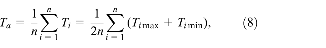
where
The OIR discrimination values that were filtered using the boxplots in Section III are used as the output from the machine learning model to characterize the battery aging level associated with the accumulated mileage.
Multiple machine learning model training, testing and comparison
Using Python 3.7, OIR estimation models based on linear regression (LR), KNN regression, support vector machine regression (SVR), random forest regression (RFR), AdaBoost regression, gradient descent tree regression (GBDT), XGboost regression, and light GBM (LGBM) regression are developed in this study. Among these approaches, the last five algorithms are integrated learning algorithms and are currently more popular, while the first three algorithms are relatively traditional, are not integrated learning algorithms, and all have different structures. The difference between the five integrated learning algorithms is that the RFR is a bagging algorithm and the rest are boosting algorithms. Among the boosting algorithms, AdaBoost differs from the rest of the algorithms in the way that it combines weak classifiers. These eight algorithms allow comparison of the applicability of the different structural algorithms to the problem of OIR estimation of real vehicles. Because all eight algorithms have been widely applied previously, their individual principles are not described in detail in this paper, but their advantages and disadvantages are listed in Table 3.
Advantages and disadvantages of the eight algorithms used for OIR estimation

The dataset of the vehicles under study was used randomly for model training and testing. The training group consists of four vehicles, and the two remaining vehicles are used as a test group to verify the validity of the trained models and also to perform model-to-model comparisons.
When the models have multiple features as inputs, they are usually min-max normalized or standardized. This procedure is followed because these multiple features often have nonuniform units and order-of-magnitude differences in their values, and models that are optimized using gradient descent algorithms have elliptical loss contours, which leads to models that are difficult or even impossible to converge, e.g. SVR models. In contrast, some KNN regression models need to calculate the distances between samples, and if the mileage of a feature is too large, it will cause the distance calculation to be mainly dependent on this feature and thus weaken the influence of the other features. However, for models with tree structures such as the RFR model, regardless of whether the characteristic data are min-max normalized or standardized, the processing has no effect. In addition, there is little difference between min-max normalization and standardization, but min-max normalization ensures that the data are strictly distributed between [0,1], which can reduce the possibility of anomalies occurring during the model training process. Therefore, the data set was min-max normalized uniformly before model training.
For models such as the RFR, AdaBoost, and GBDT models, reasonable hyper-parameters must also be set to ensure accurate estimation of the model. For example, in the RFR models, the number of decision trees, the number of randomly selected features for each decision tree, the maximum tree depth, and other hyper-parameters will all affect the final results of the model. At present, there are four major methods used to determine the hyper-parameters, i.e. the babysitting, grid, random grid, and sequential model-based Bayesian optimization methods. The random grid search method is selected for tuning of the hyper-parameters here based on the consideration that the application is likely to encounter large quantities of data in subsequent practical applications. Although the random grid search method cannot guarantee to provide the best combination of hyper-parameters, it can give a relatively good combination of hyper-parameters. Therefore, in terms of model estimation and computation time requirements, the random grid search method is the most suitable approach.
The accuracy of the model was measured using the root mean square error (RMSE), the mean absolute error (MAE), and the mean absolute percentage error (MAPE). The formulas used to calculate the RMSE, MAE, and MAPE are given in equations (9), (10), and (11), respectively.


where
Finally, the central processing unit (CPU) execution time for each model training process and prediction process is also recorded for comparison between the different models from a computational cost perspective; recording of the CPU execution time also helps to prevent the results being influenced by the other processes of the computer.
The prediction results of the different models when applied to test vehicle A are shown in Figure 7 and the corresponding results obtained for test vehicle B are shown in Figure 8. The figures show that the prediction results for the two test vehicles have relatively similar characteristics. The eight models all have relatively poor prediction results at higher OIRs (i.e. at low temperatures), which is related to the distribution of the entire data set; the city in which the vehicles are located only has low temperatures for 1 to 2 months in winter, thus resulting in fewer data being acquired for the vehicles under low temperature operating conditions. The LR and SVR predictions are comparatively worse, and their predicted values show a more obvious bias.

Prediction results of the different models when applied to the test vehicle A dataset

Prediction results of the different models when applied to the test vehicle B dataset
Table 4 shows the accuracy and computational cost results for the different models when applied to test vehicle A, and Table 5 shows the accuracy and computational cost results for the different models when applied to test vehicle B. Because the model accuracy and the computational cost are related to the data set and may be random, we have not adhered to specific rankings; instead, we have grouped the results, which may then be used as a reference for further research or applications. In terms of accuracy, for test vehicle A, the AdaBoost, GBDT, LGBM, XGBoost, and RFR models are the top five in terms of RMSE, MAE, and MAPE. For test vehicle B, the AdaBoost, GBDT, LGBM, and XGBoost models are the top four in terms of RMSE and MAE, and the GBDT, LGBM, XGBoost, and RFR models are the top four in terms of MAPE, while the AdaBoost model results are relatively average in this case. Therefore, based on the results for the accuracy for test vehicle A and test vehicle B, we recommend use of GBDT, XGBoost, and LGBM as the three models to evaluate battery aging; the AdaBoost, KNN, and RFR models can also be used as alternatives, while use of the LR and SVR models is not recommended. As shown in Table 3, the recommended GBDT, XGBoost, and LGBM approaches are all decision tree integration learning algorithms that use gradient boosting. The AdaBoost and RFR algorithms in the alternative group are also integrated learning algorithms. In terms of the computational requirements of the three recommended models (GBDT, XGBoost, and LGBM), including computation of the fitting during training and computation of the prediction after training, LGBM is better than both GBDT and XGBoost in terms of the fitting computation, and GBDT is slightly better than both XGBoost and LGBM in terms of the prediction computation; from the alternative group, KNN is better than both XGBoost and LGBM in terms of the fitting computation. In addition, in terms of the fitting computation, KNN is also significantly better than RFR and slightly better than AdaBoost, while in terms of the prediction computation, RFR is significantly better than AdaBoost and better than KNN. This can be illustrated based on the principle that the KNN algorithm is a typical inert learning algorithm; inert means that there is no explicit training data process or that this process is very fast, whereas in the prediction phase, the algorithm must still calculate the distance at each sampling instant, which can be a slow process in scenarios that involve large amounts of data and high memory requirements. Because the prediction frequency is much greater than the training frequency in practical applications (battery management system (BMS) or cloud platform), KNN prediction is too computationally intensive, which may prove disastrous for scenarios involving large amounts of data and is thus not recommended. Finally, the recommended group includes the GBDT, XGBoost, and LGBM models with an RMSE of less than 6.9 mΩ, an MAE of less than 5 mΩ, and an MAPE of less than 7.6% in the different test sets; the algorithms of the recommended group are all integrated decision tree learning algorithms that use gradient boosting, while the alternative group includes the AdaBoost and RFR models. When compared with the recommended group, the alternative group is relatively less stable, providing excellent performance for one test set and relatively poor performance for the other test set, but the group’s RMSE is less than 7.1 mΩ, the MAE is less than 5.1 mΩ, and the MAPE is less than 7.9% for the different test sets. The recommended group and the alternative group are both integrated learning algorithms, and the accuracy reported above is already relatively good when the fact that the test set used for model validation is completely different to the training set used for model training is considered. The not-recommended group includes the KNN, LR, and SVR models, where the LR and SVR are not recommended because of their poor accuracy, while the KNN is not recommended because its prediction process is highly computationally intensive, which may prove to be disastrous in application scenarios with large data volumes.
Accuracy and computational costs of the different models for the test vehicle A dataset

Accuracy and computational costs of the different models for the test vehicle B dataset

Conclusion
Based on actual operating data from purely electric passenger vehicles, this study has used multiple data-driven models to describe the relationship between the degree of battery degradation and the factors influencing this degradation. First, a DPEC model of the entire battery system was constructed and the FFRLS method was used to perform parameter identification to enable extraction of the OIR of the battery pack, which was then used to characterize the degree of degradation of the battery. Subsequently, the cumulative vehicle mileage, the average battery system temperature, the average current, the starting SOC, and the ending SOC of the driving segments were taken to be the influencing factors. The LR, KNN, SVR, RFR, Adaboost, GBDT, XGboost, and LGBM models were then trained and validated, and were tested with different datasets collected from another two purely electric passenger cars to verify the robustness of the algorithms. The results obtained show that the decision tree integrated learning algorithms, i.e. the GBDT, XGBoost, and LGBM algorithms with gradient boosting, are more accurate, with an RMSE of less than 6.9 mΩ, an MAE of less than 5 mΩ, and an MAPE of less than 7.6% for the different test sets, and these algorithms are classified as the recommended group. The other two integrated learning algorithms, AdaBoost and RFR, are relatively less stable, but their RMSE is less than 7.1 mΩ, their MAE is less than 5.1 mΩ, and their MAPE is less than 7.9% for the different test sets, and these algorithms are included in the alternative group. The LR and SVR models are not recommended because of their low accuracy, and the KNN algorithm is not recommended because of its very large prediction computation cost.
Establishing a good data-driven model on the one hand allows the problem where traditional online identification is not sufficiently stable to be effectively avoided, and on the other hand provides prediction efficiency that is high enough to be embedded into an actual battery management system or deployed on a cloud platform for real-time battery aging estimation. In addition, subsequent research or applications can refer to the grouping suggestions provided in this study to improve their model development efficiency. More vehicle types loaded with batteries composed of different materials and more algorithms will be studied and compared in future work.
Footnotes
Appendix
Abbreviations

|
|
|
|---|---|
| DPEC | Dual-polarization equivalent circuit |
| FFRLS | Forgetting factor recursive least squares |
| GBDT | Gradient boosting decision tree |
| RFR | Random forest regression |
| LR | Linear regression |
| SVR | Support vector machine regression |
| KNN | K-nearest neighbor |
| SOH | State of health |
| SOC | State of charge |
| ICA | Incremental capacity analysis |
| DVA | Differential voltage analysis |
| IC | Incremental capacity |
| ECM | Equivalent circuit model |
| OIR | Ohmic internal resistance |
| BA | Boxplot analysis |
| NCM | LiNixCoyMnzO2 |
| RC | Resistor-capacitor |
| EV | Electric vehicle |
| FNN | Fuzzy neural network |
| LSTM | Long short-term memory |
| GRU | Gated recurrent unit |
| RMSE | Root mean square error |
| MAE | Mean absolute error |
| MAPE | Mean absolute percentage error |
| CPU | Central processing unit |
| Ut | Battery terminal voltage |
| Uoc | Battery open circuit voltage |
| R0 | Battery ohmic resistance |
| RD1 | Battery electrochemical polarization resistance |
| CD1 | Battery electrochemical polarization capacitance |
| RD2 | Battery concentration difference polarization resistance |
| CD2 | Battery concentration difference polarization capacitance |
| iL | Total circuit current |
| UD1 | Voltage of the first RC circuit |
| UD2 | Voltage of the second RC circuit |
| Ia | Average current of single driving segment data |
| Ii | Current at a single sampling instant |
| Ta | Average temperature of single driving segment data |
| Ti | Temperature at a single sampling instant |
| Timax | Highest temperature at a single sampling instant |
| Timin | Lowest temperature at a single sampling instant |
| Ut | V |
| Uoc | V |
| R0 | Ω |
| RD1 | Ω |
| CD1 | F |
| RD2 | Ω |
| CD2 | F |
| iL | A |
| UD1 | V |
| UD2 | V |
| Ia | A |
| Ii | A |
| Ta | °C |
| Ti | °C |
| Timax | °C |
| Timin | °C |
| SOC | 1 |
Handling Editor: James Baldwin
Declaration of conflicting interests
The author(s) declared no potential conflicts of interest with respect to the research, authorship, and/or publication of this article.
Funding
The author(s) disclosed receipt of the following financial support for the research, authorship, and/or publication of this article: This work was supported in part by the National Key Research and Development Program of China (No. 2019YFB1600800).