An efficient technique to solve coupled–time fractional Boussinesq–Burger equation using fractional decomposition method

Abstract

For this work, a novel numerical approach is proposed to obtain solution for the class of coupled time-fractional Boussinesq–Burger equations which is a nonlinear system. This system under consideration is endowed with Caputo time-fractional derivative. By means of the natural decomposition approach, approximate solutions of the proposed nonlinear fractional system are obtained where the exact solutions are presented in the classical case of fractional order at $\gamma =1$ . Some numerical examples are given to support the theoretical framework and to point out the role and the effectiveness of the intended method. Our results clearly show the approximate analytical solutions eventually will converge quickly to the already known exact solutions.

AMS Classification: 35A22, 35C05, 35C10, 35R11, 44A30.

Introduction

It was only the starts when Leibniz sent an amazing notice to l’Hospital in 1695 which led to the theory of fractional derivatives and integrals of arbitrary order such as one-half. Since then, scholars started developing theories of fractional derivative as theoretical field of pure Mathematics for three centuries. For the past three decades, researchers started bringing the attention about non-integer fractional integrals order along with its non-integer derivatives order. Moreover, they clarify the fact that they are very useful and more adequate than classical integer order in description the properties of real materials such as polymers, modelling mechanical and electrical properties of real materials, description of archaeological properties of rocks, theory of fractals. ¹

Surveys of the history of fractional derivatives can be found in Miller and Ross, ² Podlubny, ³ Al-Smadi et al., ⁴ and Eid et al. ⁵ We can summarize all the above describing the relation between these two concepts in one sentence: fractional derivative is the generalized form of classical integer derivative. In addition, the subject of fractional derivatives can be widely applied in many real life applications, such as; engineering, mathematical biology, quantum physics, fluid mechanics fields.^6–11 Due to the fast development of software programs such as Mat Lab, Mathematica and Maple, many new powerful analytical techniques have been proposed to find new and approximate solutions for fractional linear and nonlinear differential equations such as; the sub-equation method, ¹² Exponential function method, ¹³ first integral method, ¹⁴ the expansion method, ¹⁵ fractional reproducing kernel method,^16–18 fractional Adomian decomposition method, ¹⁹ fractional homotopy perturbation, ²⁰ fractional homotopy analysis, ²¹ fractional residual power series,^22–25 fractional Laplace decomposition, ²⁶ fractional differential transform method^27–30 and other advanced numerical methods.^31–34

For the current work, an efficient method will be explored which we choose to call fractional decomposition method (FDM). It is a combination of the Adomian decomposition method and the natural transform method (NTM).^35–37 In fact, finding closed-form solutions for fractional partial differential equations is not an easy task for researchers due to the complexities of involving the fractional order. The goal of our study is to look for exact solution to coupled time-fractional fractional Boussinesq–Burger equation which is a nonlinear system using the FDM. Consider the non-linear coupled time-fractional Boussinesq–Burger equation of the form:

$$\begin{array}{c}{D}_t^{\gamma }w(x,t)+v_x(x,t)+w(x,t)w_x(x,t)=0,\hfill \\ D_t^{\gamma }v(x,t)+{\left(w(x,t)v(x,t)\right)}_x+w_{\mathrm{xxx}}(x,t)=0,\hfill \end{array}$$

(1)

along with the I.C’s

$$w(x,0)=g_1(x);v(x,0)=g_2(x).$$

(2)

In the equation above, $0<\gamma \le 1$ , $x\in [a,b]$ , $t\ge 0$ . Also, both functions $g_1(x)$ , $g_2(x)$ are analytic, and $w(x,t)$ , $v(x,t)$ are real-valued functions to be determined. Here $D_t^{\gamma }$ is for the Caputo time-fractional derivative of order $\gamma$ . We shall proceed in our paper as follow: Section 2 is intended for background of fractional calculus. In section 3 we introduce the NTM. Section 4 is devoted for the methodology of the FDM. In section 5, we give some examples of a fractional nonlinear system of differential equations. Section 6 is for discussion and conclusion of this paper.

Background of fractional calculus

In recent years, scientists showed some interest in non-local field theories and their interest really became more consistence. This development became more clear due to the expectation and the needs to use these theories so that they can treat problems in a more elegant and effective fashion. A particular group of non-local field theories plays an outstanding role and may be described with operators of fractional nature and is specified within the framework of fractional calculus.^4–9

Definition 2.1. If $m\in \mathbb{N},x>0$ with $g\in C_{-1}^m$ and $m-1<\gamma \le m$ . Then, the fractional Caputo derivative of $g$ is defined as: $D^{\gamma }g(x)=J^{m-\gamma }{D}^{m}g(x)=\frac{1}{\mathrm{\Gamma }(m-\gamma )}{\int }_0^x(x-y{)}^{m-\gamma -1}{g}^{(m)}(y)\mathrm{dy}.$

Note that, since the I.C and B.C will be included in the formulation of our applications, then the Caputo fractional derivative will be used through out the paper.

The natural transform method

Here, we refer the reader to Belgacem and Silambarasan ³⁸ to view some of the background and history of the (NTM).

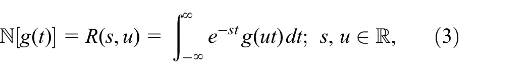
Definition 3.1. Suppose $H\left(t\right)$ is the Heaviside function. Consider a real-valued function, where the natural transform ${\mathbb{N}}^{+}$ is well-defined on the half plane $s>\mathrm{bu}$ for some $b>0$ . Let $g\left(t\right)$ be continuous on $\mathbb{R}$ . Let $K,b>0$ , then we define

$$B=\{g(t):|g(t)|<K{e}^{b\left|t\right|}H\left(t\right)+K{e}^{-b\left|t\right|}H(-t)\}.$$

Definition 3.2. The natural transform of the function $g(t)$ for $t\in \mathbb{R}$ is given by ³⁸ :

$$\mathbb{N}[g(t)]=R(s,u)={\int }_{-\infty }^{\infty }{e}^{-\mathrm{st}}g(\mathrm{ut})\mathrm{dt};s,u\in \mathbb{R},$$

(3)

where $\mathbb{N}[g(t)]$ is the natural transform of $g(t)$ .

Note that equation (3) can be written in the form ³⁸

$$\mathbb{N}[g(t)]=R^{-}(s,u)+R^{+}(s,u).$$

Definition 3.3. Suppose that $g(t)H(t)$ is defined on ${\mathbb{R}}^{+}$ , and $s,u,t\in {\mathbb{R}}^{+}$ , where $g(t)\in B$ . Then, we define the N-transform as

$$\mathbb{N}[g(t)H(t)]={\mathbb{N}}^{+}[g(t)]=R^{+}(s,u)={\int }_0^{\infty }{e}^{-\mathrm{st}}g(\mathrm{ut})\mathrm{dt}.$$

(4)

Consequently, if $u=1$ we obtain the Laplace transform and if $s=1$ , we get the Sumudu transform. Also, one can find most of the properties of the N-transforms in Rawashdeh ³⁰ and Belgacem and Silambarasan. ³⁸ For example, ${\mathbb{N}}^{+}\left[1\right]=\frac{1}{s}$ and ${\mathbb{N}}^{+}\left[t^{\gamma }\right]=\frac{\gamma !u^{\gamma }}{s^{\gamma +1}}$ , where $\gamma >-1$ .

The methodology of FDM

In this section, we give the methodology of the FDM which also can be found in Rawashdeh ³⁰ and Rawashdeh and Darweesh. ³⁵

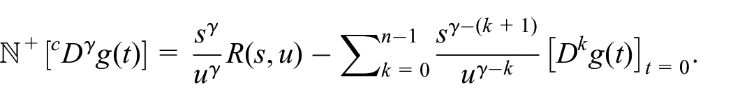
Theorem 4.1. If $m\in {\mathbb{Z}}^{+}$ , where $m-1\le \gamma <m$ and ${\mathbb{N}}^{+}[g(t)]=R^{+}(s,u)$ , then the natural transform of ${{}^{c}D}^{\gamma }g(t)$ is given by

$${\mathbb{N}}^{+}[{{}^{c}D}^{\gamma }g(t)]=\frac{s^{\gamma }}{u^{\gamma }}R(s,u)-{\sum }_{k=0}^{n-1}\frac{s^{\gamma -(k+1)}}{u^{\gamma -k}}{[D^{k}g(t)]}_{t=0}.$$

For the sake of explanation of the method algorithm, let us consider a nonlinear fractional system in the general form:

$$\begin{array}{c}{D}_t^{\gamma }v(x,t)+L_{1}v(x,t)+N_1(w,v)=g(x,t),\hfill \\ D_t^{\beta }w(x,t)+L_{2}v(x,t)+N_2(w,v)=h(x,t),\hfill \end{array}$$

(5)

along with the following initial conditions

$$\begin{array}{c}v(x,0)=g_1(x),\hfill \\ w(x,0)=g_2(x),\hfill \end{array}$$

(6)

where $D_t^{\gamma }w(x,t)$ and $D_t^{\beta }v(x,t)$ is the Caputo fractional derivative of the function $w(x,t)$ and $v(x,t)$ respectively, $L_1$ and $L_2$ are the linear differential operators, $g(x,t)$ and $h(x,t)$ are the non-homogeneous terms and $N_1(w,v)$ , $N_2(w,v)$ represent the nonlinear differential operators.

Now, by applying the ${\mathbb{N}}^{+}$ to equation (5) and theorem (4.1), we have

$$\begin{array}{c}V(x,s,u)=\frac{u^{\gamma }}{s^{\gamma }}\sum _{k=0}^{n-1}\frac{s^{\gamma -(k+1)}}{u^{\gamma -k}}{\left[D^{k}v\right]}_{t=0}\hfill \\ +\frac{u^{\gamma }}{s^{\gamma }}{\mathbb{N}}^{+}[h(x,t)]-\frac{u^{\gamma }}{s^{\gamma }}{\mathbb{N}}^{+}[L_{1}v(x,t)]-\frac{u^{\gamma }}{s^{\gamma }}{\mathbb{N}}^{+}\left[N_2(w,v)\right].\hfill \\ W(x,s,u)=\frac{u^{\beta }}{s^{\beta }}\sum _{k=0}^{n-1}\frac{s^{\beta -(k+1)}}{u^{\beta -k}}{\left[D^{k}w\right]}_{t=0}\hfill \\ +\frac{u^{\beta }}{s^{\beta }}{\mathbb{N}}^{+}[g(x,t)]-\frac{u^{\beta }}{s^{\beta }}{\mathbb{N}}^{+}[L_{2}w(x,t)]-\frac{u^{\beta }}{s^{\beta }}{\mathbb{N}}^{+}\left[N_1(w,v)\right],\hfill \end{array}$$

(7)

Thus, we apply ${\mathbb{N}}^{-1}$ to the above equation and we get

$$\begin{array}{c}\multicolumn{1}{c}{v(x,t)=K(x,t)-{\mathbb{N}}^{-1}\left[\frac{u^{\gamma }}{s^{\gamma }}{\mathbb{N}}^{+}[L_{1}v(x,t)]\right]}\\ -{\mathbb{N}}^{-1}\left[\frac{u^{\gamma }}{s^{\gamma }}{\mathbb{N}}^{+}\left[N_1(w,v)\right]\right],\hfill \\ \multicolumn{1}{c}{w(x,t)=M(x,t)-{\mathbb{N}}^{-1}\left[\frac{u^{\beta }}{s^{\beta }}{\mathbb{N}}^{+}[L_{2}w(x,t)]\right]}\\ -{\mathbb{N}}^{-1}\left[\frac{u^{\beta }}{s^{\beta }}{\mathbb{N}}^{+}\left[N_2(w,v)\right]\right].\hfill \end{array}$$

(8)

In equation (8), we have $K(x,t)$ and $M(x,t)$ are counted for both the non-homogeneous and initial conditions.

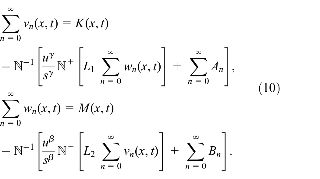
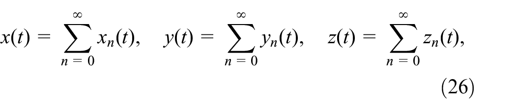
So, consider the series solutions

$$v(x,t)=\sum _{n=0}^{\infty }{v}_n(x,t);w(x,t)=\sum _{n=0}^{\infty }{w}_n(x,t).$$

(9)

From the above equation, then equation (8) becomes:

$$\begin{array}{c}\sum _{n=0}^{\infty }{v}_n(x,t)=K(x,t)\hfill \\ -{\mathbb{N}}^{-1}[\frac{u^{\gamma }}{s^{\gamma }}{\mathbb{N}}^{+}[L_1\sum _{n=0}^{\infty }{w}_n(x,t)]+\sum _{n=0}^{\infty }{A}_n],\hfill \\ \sum _{n=0}^{\infty }{w}_n(x,t)=M(x,t)\hfill \\ -{\mathbb{N}}^{-1}[\frac{u^{\beta }}{s^{\beta }}{\mathbb{N}}^{+}[L_2\sum _{n=0}^{\infty }{v}_n(x,t)]+\sum _{n=0}^{\infty }{B}_n].\hfill \end{array}$$

(10)

Looking at both sides of equation (10), one can obtain

$$\begin{array}{c}{v}_0(x,t)=K(x,t),w_0(x,t)=M(x,t),\hfill \\ v_1(x,t)=-{\mathbb{N}}^{-1}\left[\frac{u^{\gamma }}{s^{\gamma }}{\mathbb{N}}^{+}[L_1{v}_0(x,t)+A_0]\right],\hfill \\ w_1(x,t)=-{\mathbb{N}}^{-1}\left[\frac{u^{\beta }}{s^{\beta }}{\mathbb{N}}^{+}[L_2{w}_0(x,t)+B_0]\right],\hfill \\ v_2(x,t)=-{\mathbb{N}}^{-1}\left[\frac{u^{\gamma }}{s^{\gamma }}{\mathbb{N}}^{+}[L_1{v}_1(x,t)+A_1]\right],\hfill \\ w_2(x,t)=-{\mathbb{N}}^{-1}\left[\frac{u^{\beta }}{s^{\beta }}{\mathbb{N}}^{+}[L_2{w}_1(x,t)+B_1]\right].\hfill \end{array}$$

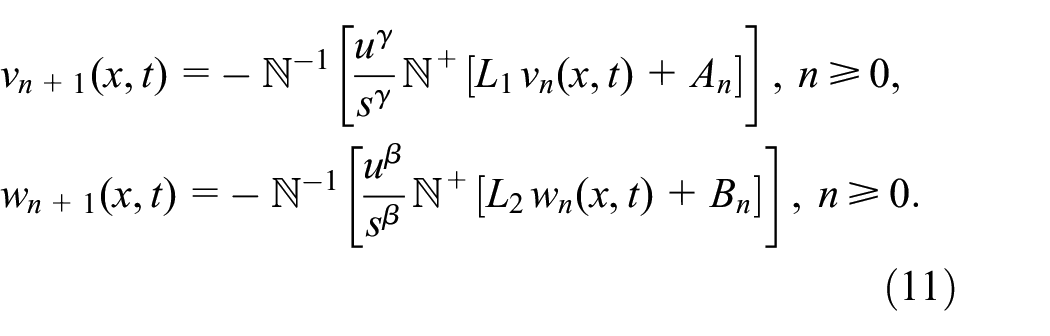
If we proceed as before one can obtain this recursive relation

$$\begin{array}{c}{v}_{n+1}(x,t)=-{\mathbb{N}}^{-1}\left[\frac{u^{\gamma }}{s^{\gamma }}{\mathbb{N}}^{+}[L_1{v}_n(x,t)+A_n]\right],n\ge 0,\hfill \\ w_{n+1}(x,t)=-{\mathbb{N}}^{-1}\left[\frac{u^{\beta }}{s^{\beta }}{\mathbb{N}}^{+}[L_2{w}_n(x,t)+B_n]\right],n\ge 0.\hfill \end{array}$$

(11)

Hence, our intended approximate solutions are as follows:

$$v(x,t)=\sum _{n=0}^{\infty }{v}_n(x,t);w(x,t)=\sum _{n=0}^{\infty }{w}_n(x,t).$$

Numerical examples

It has been demonstrated that the FDM deals efficiently with the fractional nonlinear system of differential equations when compared with the other methods that exist in literature. ³⁵ This section provides some applications of nonlinear coupled time-fractional PDEs using the FDM, including coupled Boussinesq–Burger equations which is an application of dynamical system. ³⁹

Example 1. Consider the coupled time-fractional Boussinesq–Burger equation:

$$\begin{array}{c}{D}_t^{\gamma }w(x,t)+v_x(x,t)+w(x,t)w_x(x,t)=0,(0<\gamma \le 1),\hfill \\ D_t^{\gamma }v(x,t)+{\left(w(x,y)v(x,t)\right)}_x+w_{\mathrm{xxx}}(x,t)=0,(0<\gamma \le 1),\hfill \end{array}$$

(12)

along with the I.C’s

$$w(x,0)=1+\tanh \left(\frac{x}{2}\right);v(x,0)=\frac{1}{2}-\frac{1}{2}{\tanh }^2\left(\frac{x}{2}\right).$$

(13)

According to the FDM algorithm, one can get:

$$\begin{array}{c}{\mathbb{N}}^{+}[D_t^{\gamma }w(x,t)]+{\mathbb{N}}^{+}\left[v_x(x,t)\right]+{\mathbb{N}}^{+}\left[w(x,t)w_x(x,t)\right]=0,\hfill \\ {\mathbb{N}}^{+}[D_t^{\gamma }v(x,t)]+{\mathbb{N}}^{+}\left[{\left(w(x,t)v(x,t)\right)}_x\right]+{\mathbb{N}}^{+}\left[w_{\mathrm{xxx}}(x,t)\right]=0.\hfill \end{array}$$

(14)

So equation (14) becomes

$$\begin{array}{c}\frac{s^{\gamma }}{u^{\gamma }}{\mathbb{N}}^{+}\left[w\right]-\sum _{k=0}^{n-1}\frac{s^{\gamma -(k+1)}}{u^{\gamma -k}}{\left[D^{k}w\right]}_{t=0}+{\mathbb{N}}^{+}\left[v_x\right]+{\mathbb{N}}^{+}\left[w{w}_x\right]=0,\hfill \\ \frac{s^{\gamma }}{u^{\gamma }}{\mathbb{N}}^{+}\left[v\right]-\sum _{k=0}^{n-1}\frac{s^{\gamma -(k+1)}}{u^{\gamma -k}}{\left[D^{k}v\right]}_{t=0}+{\mathbb{N}}^{+}\left[{\left(\mathrm{wv}\right)}_x\right]+{\mathbb{N}}^{+}\left[w_{\mathrm{xxx}}\right]=0.\hfill \end{array}$$

(15)

Plug equation (13) into equation (14) to conclude

$$\begin{array}{c}{\mathbb{N}}^{+}\left[w(x,t)\right]=\frac{1}{s}+\frac{1}{s}\tanh \left(\frac{x}{2}\right)-\frac{u^{\gamma }}{s^{\gamma }}{\mathbb{N}}^{+}\left[v_x\right]-\frac{u^{\gamma }}{s^{\gamma }}{\mathbb{N}}^{+}\left[w{w}_x\right],\hfill \\ {\mathbb{N}}^{+}\left[v(x,t)\right]=\frac{1}{2s}-\frac{1}{2s}{\tanh }^2\left(\frac{x}{2}\right)-\frac{u^{\gamma }}{s^{\gamma }}{\mathbb{N}}^{+}\left[{\left(\mathrm{wv}\right)}_x\right]\hfill \\ -\frac{u^{\gamma }}{s^{\gamma }}{\mathrm{N}}^{+}\left[w_{\mathrm{xxx}}\right].\hfill \end{array}$$

(16)

Now, taking the ${\mathbb{N}}^{-1}$ of the above equation, we get

$$\begin{array}{c}\multicolumn{1}{c}{w(x,t)=1+\tanh \left(\frac{x}{2}\right)-{\mathrm{N}}^{-1}\left[\frac{u^{\gamma }}{s^{\gamma }}{\mathbb{N}}^{+}\left[v_x\right]\right]}\\ -{\mathbb{N}}^{-1}\left[\frac{u^{\gamma }}{s^{\gamma }}{\mathbb{N}}^{+}\left[w{w}_x\right]\right],\hfill \\ \multicolumn{1}{c}{v(x,t)=\frac{1}{2}-\frac{1}{2}{\tanh }^2\left(\frac{x}{2}\right)-{\mathbb{N}}^{-1}\left[\frac{u^{\gamma }}{s^{\gamma }}{\mathbb{N}}^{+}\left[{\left(\mathrm{wv}\right)}_x\right]\right]}\\ -{\mathbb{N}}^{-1}\left[\frac{u^{\gamma }}{s^{\gamma }}{\mathbb{N}}^{+}\left[w_{\mathrm{xxx}}\right]\right].\hfill \end{array}$$

(17)

Consequently, let us assume the infinite series solutions of the unknown functions $w(x,t)$ , $v(x,t)$ and the nonlinear terms $w{w}_x$ , $\mathrm{wv}$ can be expanded in the forms

$$\begin{array}{c}w(x,t)=\sum _{n=0}^{\infty }{w}_n(x,t),v(x,t)=\sum _{n=0}^{\infty }{v}_n(x,t),\hfill \\ \multicolumn{1}{c}{w{w}_x=\sum _{n=0}^{\infty }{A}_n(x,t),\mathrm{wv}=\sum _{n=0}^{\infty }{B}_n(x,t).}\end{array}$$

(18)

From equations (17) and (18), we conclude that

$$\begin{array}{c}\sum _{n=0}^{\infty }{w}_n(x,t)=1+\tanh \left(\frac{x}{2}\right)-{\mathbb{N}}^{-1}\left[\frac{u^{\gamma }}{s^{\gamma }}{\mathbb{N}}^{+}\left[\sum _{n=0}^{\infty }{v}_{\mathrm{nx}}\right]\right]\hfill \\ -{\mathbb{N}}^{-1}\left[\frac{u^{\gamma }}{s^{\gamma }}{\mathbb{N}}^{+}\left[\sum _{n=0}^{\infty }{A}_n\right]\right],\hfill \\ \sum _{n=0}^{\infty }{v}_n(x,t)=\frac{1}{2}-\frac{1}{2}{\tanh }^2\left(\frac{x}{2}\right)-{\mathbb{N}}^{-1}\left[\frac{u^{\alpha }}{s^{\alpha }}{\mathbb{N}}^{+}\left[\sum _{n=0}^{\infty }{B}_{\mathrm{nx}}\right]\right]\hfill \\ -{\mathbb{N}}^{-1}\left[\frac{u^{\gamma }}{s^{\gamma }}{\mathbb{N}}^{+}\left[\sum _{n=0}^{\infty }{w}_{\mathrm{nxxx}}\right]\right].\hfill \end{array}$$

(19)

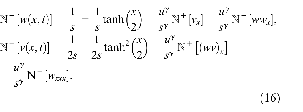
Now if we look at both sides of above equation, one can come up with:

$$\begin{array}{c}{w}_0(x,t)=1+\tanh \left(\frac{x}{2}\right),\hfill \\ v_0(x,t)=\frac{1}{2}-\frac{1}{2}{\tanh }^2\left(\frac{x}{2}\right),\hfill \\ w_1(x,t)=-{\mathbb{N}}^{-1}\left[\frac{u^{\gamma }}{s^{\gamma }}{\mathbb{N}}^{+}\left[v_{0x}\right]\right]-{\mathbb{N}}^{-1}\left[\frac{u^{\gamma }}{s^{\gamma }}{\mathbb{N}}^{+}\left[A_0\right]\right],\hfill \\ v_1(x,t)=-{\mathbb{N}}^{-1}\left[\frac{u^{\gamma }}{s^{\gamma }}{\mathbb{N}}^{+}\left[B_{0x}\right]\right]-{\mathbb{N}}^{-1}\left[\frac{u^{\gamma }}{s^{\gamma }}{\mathbb{N}}^{+}\left[w_{0\mathrm{xxx}}\right]\right].\hfill \end{array}$$

Thus, we have

$$\begin{array}{c}\multicolumn{1}{c}{w_1(x,t)=-{\mathbb{N}}^{-1}\left[\frac{u^{\gamma }}{s^{\gamma }}{\mathbb{N}}^{+}\left[v_{0x}\right]\right]-{\mathbb{N}}^{-1}\left[\frac{u^{\gamma }}{s^{\gamma }}{\mathbb{N}}^{+}\left[A_0\right]\right]}\\ \multicolumn{1}{c}{=-{\mathbb{N}}^{-1}[\frac{u^{\gamma }}{s^{\gamma }}{\mathbb{N}}^{+}(\frac{-1}{2}\sec {\mathrm{h}}^2\left(\frac{x}{2}\right)\tanh \left(\frac{x}{2}\right)}\\ -\frac{1}{2}\sec {\mathrm{h}}^2\left(\frac{x}{2}\right)+\frac{1}{2}\sec {\mathrm{h}}^2\left(\frac{x}{2}\right)\tanh \left(\frac{x}{2}\right))]\hfill \\ =-\frac{\sec {\mathrm{h}}^2\left(\frac{x}{2}\right)y^{\gamma }}{2\mathrm{\Gamma }(\gamma +1)},\hfill \end{array}$$

$$\begin{array}{c}\multicolumn{1}{c}{v_1(x,t)=-{\mathbb{N}}^{-1}\left[\frac{u^{\gamma }}{s^{\gamma }}{\mathbb{N}}^{+}\left[B_{0x}\right]\right]-{\mathbb{N}}^{-1}\left[\frac{u^{\gamma }}{s^{\gamma }}{\mathbb{N}}^{+}\left[w_{0\mathrm{xxx}}\right]\right]}\\ \multicolumn{1}{c}{=\frac{\sec {\mathrm{h}}^2\left(\frac{x}{2}\right)\tanh \left(\frac{x}{2}\right)y^{\gamma }}{2\mathrm{\Gamma }(\gamma +1)}-\frac{\sec {\mathrm{h}}^2\left(\frac{x}{2}\right)y^{\gamma }}{4\mathrm{\Gamma }(\gamma +1)}}\\ +\frac{\sec {\mathrm{h}}^2\left(\frac{x}{2}\right){\tanh }^2\left(\frac{x}{2}\right)y^{\gamma }}{4\mathrm{\Gamma }(\gamma +1)}+\frac{\sec {\mathrm{h}}^4\left(\frac{x}{2}\right)y^{\gamma }}{4\mathrm{\Gamma }(\gamma +1)}\hfill \\ \multicolumn{1}{c}{=\frac{4\csc {\mathrm{h}}^3\left(x\right){\sinh }^4\left(\frac{x}{2}\right)y^{\gamma }}{\mathrm{\Gamma }(\gamma +1)},}\end{array}$$

$$\begin{array}{c}\multicolumn{1}{c}{w_2(x,t)={\mathbb{N}}^{-1}\left[\frac{u^{\gamma }}{s^{\gamma }}{\mathbb{N}}^{+}\left[v_{1x}\right]\right]-{\mathbb{N}}^{-1}\left[\frac{u^{\gamma }}{s^{\gamma }}{\mathbb{N}}^{+}\left[A_1\right]\right]}\\ =\frac{8\csc {\mathrm{h}}^3\left(x\right){\sinh }^4\left(\frac{x}{2}\right)y^{2\gamma }}{\mathrm{\Gamma }(2\gamma +1)},\hfill \end{array}$$

and

$$v_2(x,t)=\frac{(\cosh \left(x\right)-2){\sinh }^4\left(\frac{x}{2}\right)t^{2\gamma }}{4\mathrm{\Gamma }(2\gamma +1)}.$$

By continuing in the same way, we conclude:

$$\begin{array}{c}w(x,t)=\sum _{n=0}^{\infty }{w}_n(x,t)\hfill \\ =w_0(x,t)+w_1(x,t)+w_2(x,t)+...\hfill \\ =-\frac{\sec {\mathrm{h}}^2\left(\frac{x}{2}\right)y^{\gamma }}{2\mathrm{\Gamma }(\gamma +1)}+\frac{8\csc {\mathrm{h}}^3\left(x\right){\sinh }^4\left(\frac{x}{2}\right)t^{2\gamma }}{\mathrm{\Gamma }(2\gamma +1)}+...\hfill \\ =1+\tanh \left(\frac{x-\frac{t^{\gamma }}{\gamma }}{2}\right),\hfill \end{array}$$

and

$$\begin{array}{c}\multicolumn{1}{c}{v(x,t)=\sum _{n=0}^{\infty }{v}_n(x,t)}\\ \multicolumn{1}{c}{=v_0(x,t)+v_1(x,t)+v_2(x,t)+...}\\ \multicolumn{1}{c}{=\frac{4\csc {\mathrm{h}}^3\left(x\right){\sinh }^4\left(\frac{x}{2}\right)t^{\gamma }}{\mathrm{\Gamma }(\gamma +1)}}\\ +\frac{(\cosh \left(x\right)-2){\sinh }^4\left(\frac{x}{2}\right)y^{2\gamma }}{4\mathrm{\Gamma }(2\gamma +1)}+...\hfill \\ \multicolumn{1}{c}{=\frac{1}{2}-\frac{1}{2}{\tanh }^2\left(\frac{x-\frac{t^{\gamma }}{\gamma }}{2}\right).}\end{array}$$

With the help of Taylor expansion, the intended approximate solutions for $\gamma =1$ are given by

$$\begin{array}{c}w(x,t)=1+\tanh \left(\frac{x-t}{2}\right),v(x,t)=\frac{1}{2}-\frac{1}{2}{\tanh }^2\left(\frac{x-t}{2}\right),\hfill \end{array}$$

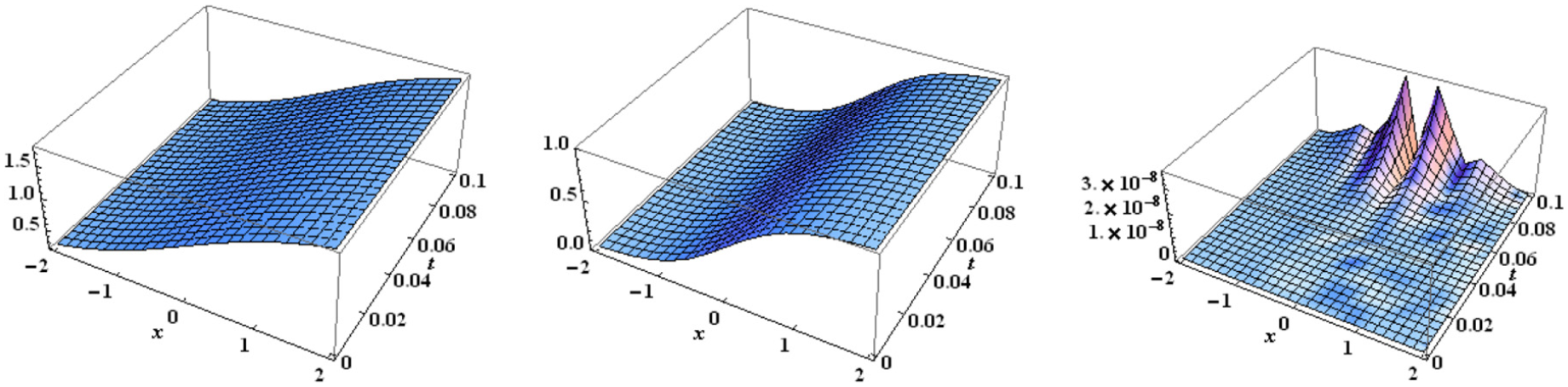
which coincides with the exact solutions of coupled time-fractional Boussinesq–Burger equations (12). In order for us, to see our proposed method (FDM) is reliable and efficient, the fractional behaviour of the approximate solutions $\{w_n(x,t),v_n(x,t)\}$ of Example 5.1 above is discussed when $n=5$ by utilizing the 2D and 3D graphs as follows: The 3D plots of $w(x,t)$ and approximate solutions $w_n(x,t)$ together with absolute error are presented in Figure 1. While the behaviour of approximate solution $w_n(x,t)$ are plotted in Figure 2 for different values of fractional order $\gamma$ such that $\gamma \in \{0.6,0.75,0.9\}$ . The 2D graphs of fractional levels of approximate solution $w_n(x,y)$ are presented in Figure 3. Similar graphical representations of approximate solution $v_n(x,t)$ are provided in Figures 4 to 6. From these graphs, it can be seen that the FDM approximations are in closed agreement with each other for various values of $\gamma$ and with exact solution.

Figure 1.

3D plots of approximate $w_5(x,t)$ , exact $w(x,t)$ and error solutions for Example 5.1.

Figure 2.

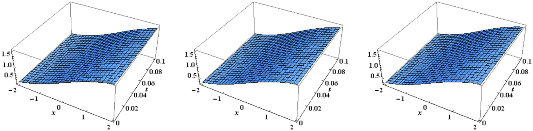
3D plots of approximate solution $w_5(x,t)$ for Example 5.1 at $\gamma =0.6$ , $\gamma =0.75$ and $\gamma =0.9$ .

Figure 3.

Fractional curves of $w_5(x,t)$ for $t=1$ , $x\in (-2,2)$ (left) and $x=2$ , $t\in [0,1]$ (right).

Figure 4.

3D plots of approximate $v_5(x,t)$ , exact $v(x,t)$ and error solutions for Example 5.1.

Figure 5.

3D plots of approximate solution $\gamma =0.75$ and $\gamma =0.9$ .

Figure 6.

Fractional curves of $v_5(x,t)$ for $t=1$ , $x\in (-2,2)$ (left) and $x=2$ , $t\in [0,1]$ (right).

Further, we can illustrate the validity of the FDM by looking at both, the exact and approximate solutions for different values of fractional order. In Tables 1 and 2, some numerical results of the approximate solutions $w(x,t)$ and $v(x,t)$ are considered at various values of $x$ and $t$ such that $x=\{-5,0,5\}$ and $t=\{0.01,0.03,0.05\}$ .

Table 1.

Numerical results of $w(x,t)$ for Example 5.1 for various values of $\gamma$ .

$x$	$t$	Exact $w(x,t)$	$w_n(x,t)$ $\gamma =1$	$\gamma =0.9$	$\gamma =0.75$	Absolute error $\gamma =1$
−5	0.01	−74.94903259	−74.94903262	−75.4373	−76.8133	$3.0980\times {10}^{-8}$
	0.03	−76.46323442	−76.46323694	−77.5719	−80.3246	$2.5195\times {10}^{-6}$
	0.05	−78.00800806	−78.00802758	−75.4373	−76.8133	$1.9519\times {10}^{-5}$
0	0.01	−0.010000166	−0.010000166	−0.01648	−0.03442	$8.3334\times {10}^{-13}$
	0.03	−0.030004500	−0.030004500	−0.04431	−0.07858	$2.0250\times {10}^{-10}$
	0.05	−0.050020833	−0.050020836	−0.07022	−0.11551	$2.6043\times {10}^{-9}$
5	0.01	73.46480888	73.46480892	72.9914	71.7047	$3.0856\times {10}^{-8}$
	0.03	72.00996962	72.00997211	70.9951	68.6619	$2.4894\times {10}^{-6}$
	0.05	70.58392112	70.58394026	69.1937	66.2551	$1.9132\times {10}^{-5}$

Table 2.

Numerical results of $v(x,t)$ for Example 5.1 for various values of $\gamma$ .

$x$	$y$	Exact $v(x,t)$	$v_n(x,t)$ $\gamma =1$	$\gamma =0.9$	$\gamma =0.75$	Absolute error $\gamma =1$
−5	0.01	74.95570350	74.95570353	75.4439	76.8199	$3.0983\times {10}^{-8}$
	0.03	76.46977323	76.46977575	77.5784	80.3309	$2.5197\times {10}^{-6}$
	0.05	78.01441739	78.01443691	79.6219	83.4055	$1.9520\times {10}^{-5}$
0	0.01	1.000050000	1.000050000	1.00015	1.00075	$4.1667\times {10}^{-10}$
	0.03	1.000450000	1.000450034	1.00108	1.00391	$3.3751\times {10}^{-8}$
	0.05	1.001250000	1.001250260	1.00271	1.00841	$2.6044\times {10}^{-7}$
5	0.01	73.47161455	73.47161458	72.9982	71.7117	$3.0859\times {10}^{-8}$
	0.03	72.01691277	72.01691526	71.0022	68.6692	$2.4896\times {10}^{-6}$
	0.05	70.59100453	70.59102367	69.2009	66.2627	$1.9134\times {10}^{-5}$

Example 2. Consider the fractional system below:

$$\begin{array}{c}{D}^{\alpha }x\left(t\right)=2y^2\left(t\right),0<\alpha \le 1,\hfill \\ D^{\beta }y\left(t\right)=tx\left(t\right),0<\beta \le 1,\hfill \\ D^{\gamma }z\left(t\right)=y\left(t\right)z\left(t\right),0<\gamma \le 1,\hfill \end{array}$$

(20)

along with the I.C’s

$$x\left(0\right)=0;y\left(0\right)=1;z\left(0\right)=1.$$

(21)

Employ the fractional N-transform algorithm on equation (20), one can conclude:

$$\begin{array}{c}{\mathbb{N}}^{+}\left[D^{\alpha }x\left(t\right)\right]=2{\mathbb{N}}^{+}\left[y^2\left(t\right)\right],\hfill \\ {\mathbb{N}}^{+}\left[D^{\beta }y\left(t\right)\right]={\mathbb{N}}^{+}\left[tx\left(t\right)\right],\hfill \\ {\mathbb{N}}^{+}\left[D^{\gamma }z\left(t\right)\right]={\mathbb{N}}^{+}\left[y\left(t\right)z\left(t\right)\right].\hfill \end{array}$$

(22)

So equation (22) becomes

$$\begin{array}{c}\frac{s^{\alpha }}{u^{\alpha }}{\mathbb{N}}^{+}\left[x\left(t\right)\right]-\sum _{k=0}^{n-1}\frac{s^{\alpha -(k+1)}}{u^{\alpha -k}}{\left[D^{(k)}x\left(t\right)\right]}_{t=0}=2{\mathbb{N}}^{+}\left[y^2\left(t\right)\right],\hfill \\ \frac{s^{\beta }}{u^{\beta }}{\mathbb{N}}^{+}\left[y\left(t\right)\right]-\sum _{k=0}^{n-1}\frac{s^{\beta -(k+1)}}{u^{\beta -k}}{\left[D^{(k)}y\left(t\right)\right]}_{t=0}={\mathbb{N}}^{+}\left[tx\left(t\right)\right],\hfill \\ \frac{s^{\gamma }}{u^{\gamma }}{\mathbb{N}}^{+}\left[z\left(t\right)\right]-\sum _{k=0}^{n-1}\frac{s^{\gamma -(k+1)}}{u^{\gamma -k}}{\left[D^{(k)}z\left(t\right)\right]}_{t=0}={\mathbb{N}}^{+}\left[y\left(t\right)z\left(t\right)\right].\hfill \end{array}$$

(23)

Combine equations (23) and (21), to accomplish

$$\begin{array}{c}{\mathbb{N}}^{+}\left[x\left(t\right)\right]=\frac{2u^{\alpha }}{s^{\alpha }}{\mathbb{N}}^{+}\left[y^2\left(t\right)\right],\hfill \\ {\mathbb{N}}^{+}\left[y\left(t\right)\right]=\frac{1}{s}+\frac{u^{\beta }}{s^{\beta }}{\mathbb{N}}^{+}\left[tx\left(t\right)\right],\hfill \\ {\mathbb{N}}^{+}\left[z\left(t\right)\right]=\frac{1}{s}+\frac{u^{\gamma }}{s^{\gamma }}{\mathbb{N}}^{+}\left[y\left(t\right)z\left(t\right)\right].\hfill \end{array}$$

(24)

Now, we take the ${\mathbb{N}}^{-1}$ of the above equation to obtain

$$\begin{array}{c}x\left(t\right)=2{\mathbb{N}}^{-1}\left[\frac{u^{\alpha }}{s^{\alpha }}{\mathbb{N}}^{+}\left[y^2\left(t\right)\right]\right],\hfill \\ y\left(t\right)=1+{\mathbb{N}}^{-1}\left[\frac{u^{\beta }}{s^{\beta }}{\mathbb{N}}^{+}\left[tx\left(t\right)\right]\right],\hfill \\ z\left(t\right)=1+{\mathbb{N}}^{-1}\left[\frac{u^{\gamma }}{s^{\gamma }}{\mathbb{N}}^{+}\left[y\left(t\right)z\left(t\right)\right]\right].\hfill \end{array}$$

(25)

Consequently, let us assume the infinite series solutions for $x(t)$ , $y(t)$ and $z(t)$ which can be written in the forms

$$x(t)=\sum _{n=0}^{\infty }{x}_n(t),y(t)=\sum _{n=0}^{\infty }{y}_n(t),z(t)=\sum _{n=0}^{\infty }{z}_n(t),$$

(26)

and the nonlinear terms $y^2\left(t\right)$ and $y\left(t\right)z\left(t\right)$ as

$$y^2\left(t\right)=\sum _{n=0}^{\infty }{A}_n(t),y\left(t\right)z\left(t\right)=\sum _{n=0}^{\infty }{B}_n(t).$$

(27)

If we combine equations (26) and (27), then equation (25) implies

$$\begin{array}{c}\sum _{n=0}^{\infty }{x}_n\left(t\right)=2{\mathbb{N}}^{-1}\left[\frac{u^{\alpha }}{s^{\alpha }}{\mathbb{N}}^{+}[\sum _{n=0}^{\infty }{A}_n(t)]\right],n\ge 0,\hfill \\ \sum _{n=0}^{\infty }{y}_n\left(t\right)=1+{\mathbb{N}}^{-1}\left[\frac{u^{\beta }}{s^{\beta }}{\mathbb{N}}^{+}\left[\sum _{n=0}^{\infty }t{x}_n\left(t\right)\right]\right],n\ge 0,\hfill \\ \sum _{n=0}^{\infty }{z}_n\left(t\right)=1+{\mathbb{N}}^{-1}\left[\frac{u^{\gamma }}{s^{\gamma }}{\mathbb{N}}^{+}[\sum _{n=0}^{\infty }{B}_n(t)]\right],n\ge 0.\hfill \end{array}$$

(28)

Now looking at equation (28), one can come up with the recursive relation

$$x_0\left(0\right)=0,y_0\left(0\right)=1,z_0\left(0\right)=1.$$

Thus,

$$\begin{array}{c}\multicolumn{1}{c}{x_1\left(t\right)=2{\mathbb{N}}^{-1}\left[\frac{u^{\alpha }}{s^{\alpha }}{\mathbb{N}}^{+}\left[A_0\left(t\right)\right]\right]=2{\mathbb{N}}^{-1}\left[\frac{u^{\alpha }}{s^{\alpha }}{\mathbb{N}}^{+}\left[{\left(y_0\right)}^2\right]\right]}\\ =\frac{2t^{\alpha }}{\mathrm{\Gamma }(\alpha +1)},\hfill \\ \multicolumn{1}{c}{y_1\left(t\right)={\mathbb{N}}^{-1}\left[\frac{u^{\beta }}{s^{\beta }}{\mathbb{N}}^{+}\left[t{x}_0\left(t\right)\right]\right]=0,}\\ \multicolumn{1}{c}{z_1\left(t\right)={\mathbb{N}}^{-1}\left[\frac{u^{\gamma }}{s^{\gamma }}{\mathbb{N}}^{+}\left[B_0\left(t\right)\right]\right]={\mathbb{N}}^{-1}\left[\frac{u^{\gamma }}{s^{\gamma }}{\mathbb{N}}^{+}\left[y_0{z}_0\right]\right]}\\ =\frac{t^{\gamma }}{\mathrm{\Gamma }(\gamma +1)},\hfill \end{array}$$

and

$$\begin{array}{c}\multicolumn{1}{c}{x_2\left(t\right)=2{\mathbb{N}}^{-1}\left[\frac{u^{\alpha }}{s^{\alpha }}{\mathbb{N}}^{+}\left[A_1\left(t\right)\right]\right]=2{\mathbb{N}}^{-1}\left[\frac{u^{\alpha }}{s^{\alpha }}{\mathbb{N}}^{+}\left[2y_0{y}_1\right]\right]=0,}\\ \multicolumn{1}{c}{y_2(t)={\mathbb{N}}^{-1}\left[\frac{u^{\beta }}{s^{\beta }}{\mathbb{N}}^{+}\left[t{x}_1\left(t\right)\right]\right]={\mathbb{N}}^{-1}\left[\frac{u^{\beta }}{s^{\beta }}{\mathbb{N}}^{+}\left[\frac{2t^{\alpha +1}}{\mathrm{\Gamma }(\alpha +1)}\right]\right]}\\ =\frac{2(\alpha +1)t^{\alpha +\beta +1}}{\mathrm{\Gamma }(\alpha +\beta +2)},\hfill \\ \multicolumn{1}{c}{z_2(t)={\mathbb{N}}^{-1}\left[\frac{u^{\gamma }}{s^{\gamma }}{\mathbb{N}}^{+}\left[B_1\left(t\right)\right]\right]={\mathbb{N}}^{-1}\left[\frac{u^{\gamma }}{s^{\gamma }}{\mathbb{N}}^{+}[y_1{z}_0+y_0{z}_1]\right]}\\ ={\mathbb{N}}^{-1}\left[\frac{u^{\gamma }}{s^{\gamma }}{\mathbb{N}}^{+}\left[\frac{t^{\gamma }}{\mathrm{\Gamma }(\gamma +1)}\right]\right]=\frac{t^{2\gamma }}{\mathrm{\Gamma }(2\gamma +1)}.\hfill \end{array}$$

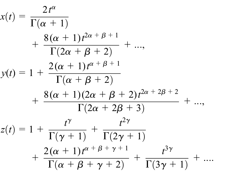
Subsequently, the 3rd approximate solutions can be obtained as

$$\begin{array}{c}{x}_3\left(t\right)=\frac{8(\alpha +1)t^{2\alpha +\beta +1}}{\mathrm{\Gamma }(2\alpha +\beta +2)},\hfill \\ y_3(t)=0,\hfill \\ z_3(t)=\frac{2(\alpha +1)t^{\alpha +\beta +\gamma +1}}{\mathrm{\Gamma }(\alpha +\beta +\gamma +2)}+\frac{t^{3\gamma }}{\mathrm{\Gamma }(3\gamma +1)}.\hfill \end{array}$$

Proceeding in this way, one comes up with these approximate solutions

$$\begin{array}{c}\multicolumn{1}{c}{x\left(t\right)=\frac{2t^{\alpha }}{\mathrm{\Gamma }(\alpha +1)}}\\ +\frac{8(\alpha +1)t^{2\alpha +\beta +1}}{\mathrm{\Gamma }(2\alpha +\beta +2)}+...,\hfill \\ \multicolumn{1}{c}{y(t)=1+\frac{2(\alpha +1)t^{\alpha +\beta +1}}{\mathrm{\Gamma }(\alpha +\beta +2)}}\\ +\frac{8(\alpha +1)(2\alpha +\beta +2)t^{2\alpha +2\beta +2}}{\mathrm{\Gamma }(2\alpha +2\beta +3)}+...,\hfill \\ \multicolumn{1}{c}{z\left(t\right)=1+\frac{t^{\gamma }}{\mathrm{\Gamma }(\gamma +1)}+\frac{t^{2\gamma }}{\mathrm{\Gamma }(2\gamma +1)}}\\ +\frac{2(\alpha +1)t^{\alpha +\beta +\gamma +1}}{\mathrm{\Gamma }(\alpha +\beta +\gamma +2)}+\frac{t^{3\gamma }}{\mathrm{\Gamma }(3\gamma +1)}+....\hfill \end{array}$$

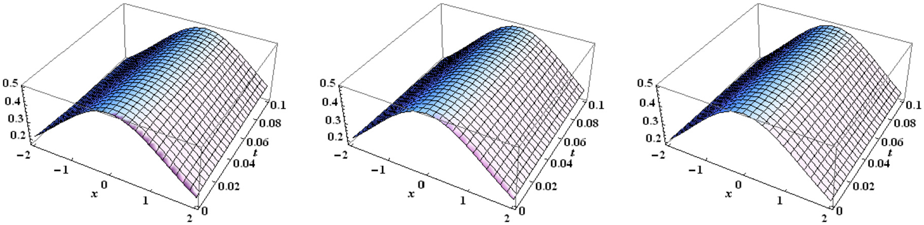
For graphical representation, 2D plots of approximate solutions $x(t)$ , $y(t)$ and $z(t)$ are respectively presented in Figures 7 to 9 for $0\ge t\ge 1.5$ and different fractional order $\alpha ,\beta ,\gamma =\{0.6,0.75,0.9,1\}$ .

Figure 7.

Fractional curves for $x(t)$ in Example 2.

Figure 8.

Fractional curves for $y(t)$ in Example 2.

Figure 9.

Fractional curves for $z(t)$ in Example 2.

Clearly, from Figures 7 to 9, the FDM exact and approximation solutions are in close agreement for various values of fractional order. Hence, the approximate solution is convergent fast enough to the exact solution.

Conclusion

We successfully employed the The fractional decomposition method and we obtained analytical approximate and exact solutions for two time-fractional order nonlinear systems. We were being able to find exact solutions to nonlinear system of coupled time-fractional Boussinesq–Burger equation. To the best of our knowledge, we are the first to find such exact solutions for the proposed systems. Since the exact solutions of most FDE’s cannot be found easily, then analytical and numerical methods like (FDM) can be used more often. In all cases, the (FDM) provided us with exact solutions in the case when $\gamma =1$ . The results showed that (FDM) is simple and easy mathematical technique to accomplish exact and numerical solutions of nonlinear time-fractional equations. Finally, one can conclude the FDM can be employ to investigate and study numerous applications of fractional differential equations which usually shows up in many areas of Physics and engineering.

References

1.
MandelbrotB. The fractal geometry of nature. San Francisco: Freeman, 1982.
2.
MillerKSRossB. An introduction to the fractional calculus and fractional differential equations. New York, NY: John Wiley and Sons Inc., 1993.
Al-SmadiMAbu ArqubOHadidS. Approximate solutions of nonlinear fractional Kundu-Eckhaus and coupled fractional massive thirring equations emerging in quantum field theory using conformable residual power series method. Phys Scr2020; 95(10): 105205.
5.
EidRMuslihSIBaleanuD, et al. On fractional Schrödinger equation in -dimensional fractional space. Nonlinear Anal Real World Appl2009; 10(3): 1299–1304.
6.
Al-SmadiMAbu ArqubOHadidS. An attractive analytical technique for coupled system of fractional partial differential equations in shallow water waves with conformable derivative. Commun Theor Phys2020; 72(8): 085001.
7.
TalafhaAGAlqaralehSMAl-SmadiM, et al. Analytic solutions for a modified fractional three wave interaction equations with conformable derivative by unified method. Alex Eng J2020; 59(5): 3731–3739.
BaleanuDFernandezA. On some new properties of fractional derivatives with Mittag-Leffler kernel. Commun Nonlinear Sci Numer Simul2018; 59: 444–462.
10.
BaleanuDMachadoJATLuoAC. Fractional dynamics and control. Berlin: Springer, 2012.
11.
Al-SmadiMAbu ArqubOGaithM. Numerical simulation of telegraph and Cattaneo fractional-type models using adaptive reproducing kernel framework. Math Methods Appl Sci. Epub ahead of print 3December2020. DOI: 10.1002/mma.6998.
12.
GuoSMeiLLiY, et al. The improved fractional sub-equation method and its applications to the space-time fractional differential equations in fluid mechanics. Phys Lett A2012; 376: 407–411.
13.
ZhangSZongQ-ALiuD, et al. A generalized exp-function method for fractional Riccati differential equations. Commun Fract Calc2010; 1: 48–51.
14.
LuB. The first integral method for some time fractional differential equations. J Math Anal Appl2012; 395: 684–693.
15.
ZhengB. -expansion method for solving fractional partial differential equations in the theory of mathematical physics. Commun Theor Phys2012; 58: 623–630.
16.
HasanSEl-AjouAHadidS, et al. Atangana-Baleanu fractional framework of reproducing kernel technique in solving fractional population dynamics system. Chaos Solitons Fractals2020; 133: 109624.
17.
Al-SmadiMAbu ArqubO. Computational algorithm for solving fredholm time-fractional partial integrodifferential equations of dirichlet functions type with error estimates. Appl Math Comput2019; 342: 280–294.
18.
Al-SmadiM. Simplified iterative reproducing kernel method for handling time-fractional BVPs with error estimation. Ain Shams Eng J2018; 9(4): 2517–2525.
19.
AbassyTA. New treatment of adomian decomposition method with compaction equations. Stud Nonlinear Sci2010; 1(2): 41–49.
20.
AbdulazizOHashimIMomaniS. Solving systems of fractional differential equations by homotopy-perturbation method. Phys Lett A2008; 37(4): 451–459.
21.
PandeyRKMishraHK. Homotopy analysis Sumudu transform method for time-fractional third order dispersive partial differential equation. Adv Comput Math2017; 43: 365–383.
22.
Al-SmadiMAbu ArqubOMomaniS. Numerical computations of coupled fractional resonant Schrödinger equations arising in quantum mechanics under conformable fractional derivative sense. Phys Scr2020; 95(7): 075218.
23.
FreihetAHasanSAl-SmadiM, et al. Construction of fractional power series solutions to fractional stiff system using residual functions algorithm. Adv Differ Equ2019; 2019: 95.
24.
HasanSAl-SmadiMFreihetA, et al. Two computational approaches for solving a fractional obstacle system in Hilbert space. Adv Differ Equ2019; 2019: 55.
25.
FreihetAShathaHAlaroudM, et al. Toward computational algorithm for time-fractional Fokker-Planck models. Adv Mech Eng2019; 11(10): 1–10.
26.
KazemS. Exact solution of some linear fractional differential equations by laplace transform. Int J Nonlinear Sci2013; 16: 3–11.
27.
RawashdehM. A new approach to solve the fractional harry dym equation using the FRDTM. Int J Pure Appl Math2014; 95(4): 553–566.
28.
Al-SmadiMFreihatAKhalilA, et al. Numerical multistep approach for solving fractional partial differential equations. Int J Comput Methods2017; 14(3): 1750029.
29.
RawashdehM. A reliable method for the space-time fractional Burgers and time-fractional Cahn-Allen equations via the FRDTM. Adv Differ Equ2017; 2017: 99.
30.
RawashdehM. An Efficient approach for time-fractional Damped Burger and time-Sharma-Tasso-Olver equations using the FRDTM. Appl Math Inf Sci2015; 9(3): 1239–1246.
31.
RawashdehM. The fractional natural decomposition method: theories and applications. Math Methods Appl Sci2017; 40(7): 2362–2376.
32.
KhanHChuYMShahR, et al. Exact solutions of the Laplace fractional boundary value problems via natural decomposition method. Open Phys2020; 18(1): 1178–1187.
33.
HasanSAl-SmadiMEl-AjouA, et al. Numerical approach in the Hilbert space to solve a fuzzy Atangana-Baleanu fractional hybrid system. Chaos Solitons Fractals2021; 143: 110506.
34.
EltayebHAbdallaYTBacharI, et al. Fractional telegraph equation and its solution by natural transform decomposition method. Symmetry2019; 11(3): 334.
35.
RawashdehMSDarweeshAH. A novel approach for finding approximate solutions of fractional systems of linear partial differential equations using the fractional natural decomposition method. Int J Multiscale Comput Eng2019; 17(5): 507–527.
36.
RawashdehMAl-JammalH. New approximate solutions to fractional nonlinear systems of partial differential equations using the FNDM. Adv Differ Equ2016; 2016: 235.
37.
RawashdehMAl-JammalH. Numerical solutions for systems of nonlinear fractional ordinary differential equations using the FNDM. Mediterr J Math2016; 13: 4661–4677.
38.
BelgacemFBMSilambarasanR. Theory of natural transform. Math Eng Sci Aerosp2012; 3: 99–124.
39.
KhaterMMAKumarD. New exact solutions for the time fractional coupled Boussinesq-Burger equation and approximate long water wave equation in shallow water. J Ocean Eng Sci2017; 2(3): 223–228.