Sage Journals: Discover world-class research

Abstract

Fault diagnosis is of great significance to improve the production efficiency and accuracy of industrial robots. Compared with the traditional gradient descent algorithm, the extreme learning machine (ELM) has the advantage of fast computing speed, but the input weights and the hidden node biases that are obtained at random affects the accuracy and generalization performance of ELM. However, the level-based learning swarm optimizer algorithm (LLSO) can quickly and effectively find the global optimal solution of large-scale problems, and can be used to solve the optimal combination of large-scale input weights and hidden biases in ELM. This paper proposes an extreme learning machine with a level-based learning swarm optimizer (LLSO-ELM) for fault diagnosis of industrial robot RV reducer. The model is tested by combining the attitude data of reducer gear under different fault modes. Compared with ELM, the experimental results show that this method has good stability and generalization performance.

Keywords

Industrial robots fault diagnosis extreme learning machine level-based learning swarm optimizer attitude sensors

Introduction

In recent years, the number and use time of industrial robots have continuously increased, leading to an increase in fault frequency. For continuous production systems, it is of great significance to carry out the fault diagnosis of industrial robots to improve their reliability.¹ The rapid identification of fault types is beneficial to the improvement of production efficiency of industrial robots in the field of application, loading and unloading.

Many researchers have focused on the application of machine learning methods such as support vector machines,² convolutional neural networks,³ deep belief networks,⁴ and sparse autoencoders⁵ in the field of fault diagnosis. Wu et al.⁶ proposed a convolutional neural network algorithm for end-to-end fault diagnosis. Zhang et al.⁷ proposed deep fuzzy echo state networks and a deep hybrid state network for machinery fault diagnosis. Isham et al.⁸ put forward a parameter optimization method for variational mode decomposition using a differential evolution algorithm for multi-fault identification. Wang et al.⁹ combined transient modelling and parameter identification to detect the fault characteristics of rotating machines. Luo et al.¹⁰ presented a hybrid system for the fault diagnosis of rolling element bearings. Zhang et al.¹¹ proposed a residual learning algorithm to improve the network training for the fault diagnosis of rotating machinery. Li et al.¹² combined variational mode decomposition and a deep neural network for the fault diagnosis of planetary gears. Zheng et al.¹³ established a variable prediction model for rolling bearing fault feature classification.

In terms of the fault diagnosis of industrial robots, Jaber et al.¹⁴ used a time-frequency signal analysis method based on the discrete wavelet transform to extract the most significant features related to faults and used an artificial neural network to perform fault classification. Freyermuth¹⁵ proposed a method for the early diagnosis of mechanical faults in industrial robots in the form of nonlinear differential equations. Anand et al.¹⁶ proposed a method for the fault detection and isolation of industrial robots based on hybrid intelligence.

Because gradient learning algorithms with a complex iterative process are used to train neural networks, the training speed of deep neural networks is generally low. To address this problem, Huang et al.¹⁷ proposed the extreme learning machine (ELM), which uses the Moore-Penrose generalized inverse to calculate the output weights after random selection of the input weights and hidden biases. It has a good learning speed performance¹⁸ and can overcome disadvantages such as local minimization, an inappropriate learning rate, and the overfitting of traditional feedforward neural networks. However, compared with the traditional gradient descent algorithm, the ELM uses many hidden nodes.¹⁹

The use of an ELM for fault diagnosis faces two major challenges: (1) random network parameters lead to poor generalization performance, (2) the model falls into overfitting due to the existence of redundant hidden nodes.²⁰ Evolutionary algorithms have been used in many studies to improve the conditions of ELM parameters. Gao et al.²¹ proposed a method for the mechanical fault diagnosis of high-voltage circuit breakers based on hybrid feature extraction and integrated ELM (IELM). Chen et al.²² used a summation wavelet ELM (SW-ELM) for fault classification and location estimation. Rodriguez et al.²³ combined an ELM and stationary wavelet transform to perform rolling bearing fault diagnosis. Chen et al.²⁴ used complementary ensemble empirical mode decomposition and an ELM to propose a fault diagnosis method suitable for engineering applications.

ELMs have been optimized with algorithms including particle swarm optimization (PSO),²⁵ competitive swarm optimization (CSO),²⁶ and differential evolution (DE).²⁷ Xu and Shu²⁸ proposed an ELM model based on PSO evolution. Eshtay et al.²⁹ presented a CSO-ELM, which uses CSO to optimize the parameters of the classical ELM and a regularized ELM for medical classification problems. Zhu et al.³⁰ put forward a new ELM that uses DE to select input weights and shows a good generalization performance. Cao et al.³¹ proposed an improved crow search algorithm to optimize the extreme learning machine. Wen³² put forward ant colony optimization algorithm and extreme learning machine network for wind turbine.

The fault diagnosis of industrial robot RV reducer is a complex problem, and ELMs require a large number of parameters to solve problems. However, for ELMs with a complex network structure, there are still problems such as slow learning speeds and poor stability. In this paper, the main contributions of this work include: (1) this work adopts low-cost attitude sensor for data acquisition; (2) a new method of level-based learning swarm optimizer with extreme learning machine (LLSO-ELM), which uses LLSO to quickly obtain the optimal input weights and hidden biases of ELM; (3) compared with ELM algorithm, this method has high prediction accuracy and generalization performance for attitude data of industrial robots under different fault modes.

The remainder of the paper is organized as follows. Section 2 introduces the proposed LLSO-ELM algorithm, Section 3 describes the experimental setup and data processing, Section 4 discusses the experimental results, and Section 5 summarizes the findings.

Methods

Extreme learning machine

ELMs are fast learning algorithms for single hidden layer feedforward neural networks.³³ Different from the back propagation algorithm based on neural networks, ELMs randomly select the input weights and hidden biases and then calculate the output weights using the Moore-Penrose generalized inverse; hence ELMs have a faster training speed. Their architecture is shown in Figure. 1.

Figure 1.

The ELM framework.

For a classification problem, it is assumed that an n-dimensional dataset has N samples, which can be divided into m categories. The training sample is set to $(X, T) = {(x_{i}, t_{i})} (i = 1, \dots, N)$ , which is input to the neural network; x_i ( $x_{i} = {[x_{i 1}, x_{i 2}, \dots, x_{in}]}^{T}$ , i = 1,…, N) is the ith input data; and t_i ( $t_{i} = {[t_{i 1}, t_{i 2}, \dots, t_{im}]}^{T}$ , i = 1,…, N) is the ith target data. The output model of the ELM neural network is as follows:

Y_{i} = \sum_{i = 1}^{L} G_{i} (X) \cdot β_{l}

(1)

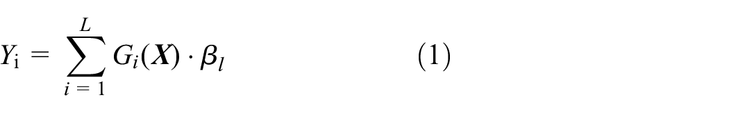
where L is the number of hidden neurons, and β _l ( $β_{l} = {[β_{l 1}, β_{l 2}, \dots, β_{lm}]}^{T}$ ) is the weight parameters vector between the lth hidden node and the output layer. G _i is the feature map, which actually maps the data from the N-dimensional input space to the L-dimensional hidden layer feature space G. The function of G _i is as follows:

G_{i} (x) = g (w_{l} x_{i} + b_{l})

(2)

where g is an activation function, w_l ( $w_{l} = {[w_{l 1}, w_{l 2}, \dots, w_{\ln}]}^{T}$ ) is the weight parameters vector connecting the nodes of the input layer and the lth hidden layer, and b _l is the node bias of the lth hidden layer. It should be noted that w_l and b _l are randomly generated. For high-precision models, Y_i = t_i can be generally considered. Then, according to Figure 1, the output matrix of the network can be obtained as

H β = T

(3)

H = {[\begin{matrix} g (α_{1} x_{1} + b_{1}) & \dots & g (α_{L} x_{1} + b_{L}) \\ ⋮ & ⋱ & ⋮ \\ g (α_{1} x_{N} + b_{1}) & \dots & g (α_{L} x_{N} + b_{L}) \end{matrix}]}_{N \times L}

(4)

β = {[β_{1} \dots β_{L}]}_{L \times m}^{T}

(5)

T = {[t_{1} \dots t_{N}]}_{N \times m}^{T}

(6)

The loss function can be described as below:

‖ H β^{'} - T ‖ = \min ‖ H β - T ‖

(7)

Because the input weight α and the hidden layer node bias b have been randomly determined, the output weight matrix $β'$ can be calculated use the least square method, as expressed below:

β' = {(H^{T} H)}^{- 1} H^{T} T

(8)

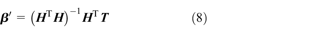
where H is the hidden layer output matrix, and T is the target matrix.

Level-based learning swarm optimizer algorithm

When solving large-scale optimization problems, optimization algorithms are prone to fall into local optimality and premature convergence. The LLSO proposed in 2017 can effectively search for the global optimal solution for large-scale problems.³⁴ The LLSO has two main ideas, namely, a level-based learning (LL) strategy and paradigm selection. The particles in the social learning particle swarm optimization (SL-PSO) algorithm³⁵ are sorted according to their fitness values and then divided into NL levels using the LL strategy. The better particles have higher levels, and their corresponding levels have smaller subscripts. If L_i represents the ith layer, L₁ is the highest layer containing the best particles. Higher-level particles may contain more useful information, which can be used to guide the lower-level particles to search for the global optimal region. Assuming that the size of the particle swarm is NP, the number of particles per layer is LS, then the total number of layers is NL = NP/LS, and the dimension is D. The architecture for the LL strategy is shown in Figure 2. First the particle swarm is sorted in ascending order of fitness, then the particle swarm is divided into NL levels, and finally particles of level L_i ( $2 \leq i \leq NL - 1$ ) are updated by learning from the particles of levels L₁ to L_i-1.

Figure 2.

Schematic architecture of the LL strategy.

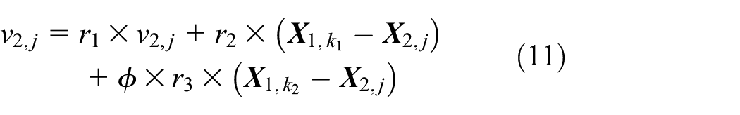
Low-level particles need to learn from high-level particles. A key problem is how to select two paradigms at higher levels. The paradigm selection strategy provides a method for selecting paradigms and considers the exploration and exploitation of particles, which are two key evaluation indicators of large-scale optimization.³⁶ The process of paradigm selection for particles of level L_i is summarized as follows: (1) randomly select rl₁ and rl_2, where $r l_{1}, r l_{2} \in [1, i - 1]$ ; (2) if $r l_{1} > r l_{2}$ , exchange their values; (3) randomly select k₁ and k₂, $k_{1}, k_{2} \in [1, LS]$ ; (4) return the k₁th particle in level rl ( $X_{r l_{1}, k_{1}}$ ) and the k₂th particle in level rl₂ ( $X_{r l_{2}, k_{2}}$ ). In the learning process, the paradigms ${X_{r l_{1}}}_{,_{k_{1}}}$ and ${X_{r l_{2}}}_{, k_{2}}$ will guide the evolution of particles in level L_i. Therefore, the updating particle X_{i, j} in the LLSO is as follows:

\begin{matrix} v_{i, j} = r_{1} \times v_{i, j} + r_{2} \times (X_{r l_{1}, k_{1}} - X_{i, j}) \\ + ϕ \times r_{3} \times (X_{r l_{2}, k_{2}} - X_{i, j}) \end{matrix}

(9)

X_{i, j} = X_{i, j} + v_{i, j}

(10)

where X_{i, j} is the jth particle in L_i, and v_{i, j} is its velocity. ${X_{r l_{1}}}_{,_{k_{1}}}$ and ${X_{r l_{2}}}_{, k_{2}}$ are determined by the paradigm selection strategy. The parameters r₁, r₂, and r₃ are randomly selected within [0, 1]. ϕ is a control parameter that determines the influence of the second paradigm, and its value is also within the range of [0, 1]. When the particle in L₂ is updated, both examples are selected from L₁, and the formula for particle updating in L₂ is as follows:

\begin{matrix} v_{2, j} = r_{1} \times v_{2, j} + r_{2} \times (X_{1, k_{1}} - X_{2, j}) \\ + ϕ \times r_{3} \times (X_{1, k_{2}} - X_{2, j}) \end{matrix}

(11)

X_{2, j} = X_{2, j} + v_{2, j}

(12)

The particles in L₁ contains the best solutions in the swarm, so they directly enter the next generation swarm. In the LLSO algorithm, good particles are retained to be learned, and bad particles are allowed to explore, which not only maintains the diversity but also accelerates the convergence of the particles and achieves large-scale optimization.

As the simplicity of particle swarm optimization algorithm is maintained in LLSO, the time complexity of LLSO calculation is very simple. First it takes O (NPlog(NP)+NP) to sort the swarm and divide the swarm into NL levels for each generation. It takes O (NP×D) to update particles in all levels except those in the first level that go directly to the next generation. In terms of space complexity, LLSO requires much less space than PSO because it does not store a personal optimal position for each particle, which takes O (NP×D) space. In conclusion, compared with the classical particle swarm optimization algorithm, LLSO maintains a higher computational efficiency in both time and space.

LLSO-ELM algorithm

In ELMs, the input weights and hidden biases are randomly selected. Random parameters can lead to more hidden neurons and poorer generalization performance. Therefore, we propose a hybrid LLSO-ELM method, which is achieved by using the LLSO to search for the optimal parameters of the ELM. Because of the full connection mode between the input layer and the hidden layer in the ELM, weight and bias optimization are a large-scale optimization problem. The LLSO has been convincingly verified in solving large-scale optimization problems.

Particle encoding and fitness are two key issues in the optimization of the ELM parameters by the LLSO. In the LLSO-ELM, particles are composed of the weight vector of the input layer and the bias vector of the hidden neurons. A particle P can be expressed as

P = [w_{11}, w_{12}, \dots, w_{1 L}, \dots w_{n 1}, \dots w_{nL}, b_{1}, \dots b_{L}]

(13)

where L is the number of hidden neurons, and n is the dimension of the input dataset. The length of the particle, LenOfParticle, can be expressed as

LenofParticle = (n + 1) \times L

(14)

Fitness is used to evaluate the quality of particles. The smaller the value, the better the classification effect. For classification problems, the fitness value can be calculated by the following formula:

Fitness = 1 - Acc

(15)

where Acc refers to the ratio between the number of correctly classified samples and the total number of samples obtained by using ELM algorithm classification after the LLSO algorithm seeks for the optimal parameters.

Basic flowchart of the LLSO-ELM algorithm

The specific flowchart of the LLSO-ELM algorithm is shown in Figure 3. The overall steps are as follows:

Step 1. Random initialization of the particle swarm of the LLSO. Each particle is composed of the input weight and the hidden bias and is valuated in the range of [−1, 1].

Step 2. Calculate the fitness value of each particle. The ELM is constructed using the correlation variables of the particles, and then the output weights are calculated to obtain the corresponding Acc.

Step 3. Update the low-level particle swarm and repeat Steps 2 and 3 according to the predetermined number of iterations.

Step 4: The optimal particles generated in the ELM in the above steps are input to the experimental data, to obtain the prediction accuracy of the proposed method.

Figure 3.

Flowchart of the LLSO–ELM algorithm.

Experiment and data processing

To verify the effectiveness of the proposed LLSO-ELM algorithm, the RV reducer gear of the industrial robot is selected to work under different fault conditions, and attitude sensors are used to collect data from the industrial robot. The experimental setup is shown in Figure 4. An industrial robot (BRTIRUS1510A) with an RV reducer gear (Qinchuan) was used in the experiment.

Figure 4.

Experimental setup.

The industrial robot is mainly used in the industrial fields of loading and unloading and injection moulding, which has a maximum load capacity of 10 kg and a maximum arm length of 1500 mm. The robot has six degrees of freedom and is composed of a pedestal, upper arms, elbows, and forearms. An RV reducer gear is installed at each joint for drive. On axis J2, the RV reducer gear is connected to the pedestal and upper arm of the robot, respectively. The sun gear is connected to the motor on one end and meshed with the planetary gear on the other end, so that the motor drives the rotation of the forearm. Similarly, the reduction gear on axis J3 is installed in the same way as that on axis J2.

The attitude data of the six-axis industrial robot is collected through attitude sensors, which can measure three-axis acceleration, three-axis angular velocity, three-axis magnetic field, and three-axis angle signals and can operate at 40–80°C. The attitude sensors have an acceleration resolution of 0.01 g, an angular velocity stability of 0.05°/s, and a sampling frequency of 100 Hz. The attitude sensors are installed on axes J1 and J6 of the robot, respectively.

The fault components of the industrial robot are the gears of the J2 and J3 axis reduction gears. The most common faults during the gear drive process are pitting faults, broken tooth faults, and crack faults. In our scheme, to simulate different fault modes, the sun gear and planetary gear on axes J2 and J3 of the industrial robot were preset with different faults, which were used as failure modes, as shown in Figure 5. Table 1 lists a total of six failure modes that were set in this study, including normal, broken tooth of the sun gear on axis J2, crack of the planetary gear on axis J2, broken tooth of the planetary gear on axis J2, pitting of the sun gear on axis J3, broken tooth of the sun gear on axis J3, and crack of the planetary gear on axis J3.

Figure 5.

Fault modes of the RV reduction gear: (a) normal planetary gear, (b) planetary gear with crack, (c) planetary gear with broken tooth, (d) normal sun gear, (e) sun gear with broken tooth, and (f) sun gear with pitting.

Table 1.

Failure modes setting the experiment.

Pattern no.	Fault axis	Fault situation	Degree of fault
A	Normal	Normal	Normal
B	J2	Sun gear	Full broken tooth
C	J2	Planetary gear	Crack (width 0.5 mm, depth 0.5 mm)
D	J2	Planetary gear	Full broken tooth
E	J3	Sun gear	Moderate pitting
F	J3	Sun gear	Full broken tooth
G	J3	Planetary gear	Crack (width 0.5 mm, depth 0.5 mm)

In the experiment, the robot was set up with a fixed trajectory using a teach pendant, with the rotation set to a low speed (600 r/min) and the load set to a heavy load (9.6 kg). In each experiment, the coordinates of the industrial robot were first zeroed. Each axis was then moved back and forth three times within a set range of angles in turn, and each experiment was repeated 10 times. To better analyse and compare the effectiveness of the proposed algorithm, different fault modes were combined. To compare the classification effects of different fault types, the classification patterns are described as follows. There are three types of ABC pattern (defined as C3), four types of ADEF pattern (defined as C4), five types of ABCDE pattern (defined as C5), and seven types of ABCDEFG pattern (defined as C7). At the end of an experiment, the data from the attitude sensors at the six axis ends were simply processed, that is, one data point was taken every 200 points. Finally, a total of 6480 samples were collected for each pattern, with nine channels of data for each sample. In the subsequent fault diagnosis experiment, the entire dataset was divided into two parts: the training dataset (80%) and the test dataset (20%).

Experimental results and discussion

Each type of dataset was trained and tested nine times. Through parameter setting experiments, the parameters of the LLSO-ELM were set as NP = 100, NL = 10, LS = 10, MAX_FIT = 4510, ϕ = 0.5, and L = 80. The prediction accuracy of each dataset is shown in Table 2 and Figure 6. As seen, the LLSO-ELM has a higher prediction accuracy than the ELM for most of the datasets and a lower accuracy only for very few cases, but the difference between the two is very small. Therefore, the LLSO-ELM method has a high classification accuracy and a stable performance.

Table 2.

Prediction accuracy comparison of the LLSO-ELM and ELM methods for each dataset.

Method	Dataset	Running order									Mean	Variance
Method	Dataset	1st	2st	3st	4st	5st	6st	7st	8st	9st	Mean	Variance
LLSO–ELM	C3	0.958	0.958	0.958	0.900	0.967	0.967	0.967	0.983	0.958	0.957	0.023
	C4	0.894	0.913	0.956	0.906	0.931	0.925	0.925	0.919	0.963	0.926	0.022
	C5	0.835	0.910	0.835	0.890	0.870	0.910	0.875	0.870	0.920	0.879	0.031
	C7	0.789	0.825	0.846	0.832	0.804	0.811	0.789	0.793	0.804	0.810	0.020
ELM	C3	0.950	0.925	0.925	0.933	0.942	0.925	0.925	0.958	0.942	0.936	0.013
	C4	0.897	0.889	0.902	0.884	0.881	0.884	0.878	0.880	0.892	0.887	0.008
	C5	0.820	0.785	0.810	0.785	0.815	0.800	0.880	0.775	0.835	0.812	0.010
	C7	0.629	0.636	0.682	0.679	0.643	0.671	0.671	0.632	0.714	0.662	0.029

Figure 6.

Result comparison of the LLSO–ELM and ELM methods for each dataset.

To demonstrate the superiority of the proposed LLSO-ELM, we compared it with the ELM. There is no empirical rule for setting the number of hidden neurons in an ELM. For comprehensive comparison, we conducted experiments by changing the number of hidden neurons in the LLSO-ELM and the ELM. In the experiment, each algorithm started with 50 hidden neurons, and 10 more hidden neurons were added each time until the number of hidden neurons reached 100, when the experiment ended. Both algorithms were run in the same operating environment as described above. Figure 7 shows the average prediction accuracies of the LLSO-ELM and the ELM with different numbers of hidden neurons for each dataset. It can be seen that the proposed LLSO-ELM outperforms the ELM for each number of hidden nodes. In addition, the prediction accuracy of the LLSO-ELM exceeds 78%, so the LLSO-ELM has a more stable performance.

Figure 7.

The average prediction accuracies of the LLSO–ELM and the ELM with different hidden neurons for each dataset: (a) C3, (b) C4, (c) C5, and (d) C7.

Conclusion

The LLSO-ELM method has been proposed in this study for the mechanical fault diagnosis of industrial robot reducer gear. To further improve the generalization performance of ELMs, we have designed the LLSO-ELM model and used the LLSO to optimize the input weights and hidden layer biases of the ELM. The experimental setup consisted of a six-axis industrial robot, attitude sensors, and other components and was mainly used to collect the attitude data of the industrial robot in different working modes. Furthermore, these attitude data were combined into a variety of datasets to analyse the performance of the LLSO-ELM and compare it with that of the ELM. The experimental results have shown that the proposed LLSO-ELM algorithm has a high prediction accuracy for the fault diagnosis of reducer gear in six-axis industrial robots, and it also has a stable performance when set up with different numbers of hidden neurons, which is of great significance for further research on other parts of industrial robots.

In the future research, we will further combine the ELM algorithm with other metaheuristic algorithms for comparison, such as ant colony, monarch butterfly optimization (MBO), earthworm optimization algorithm (EWA) and other optimized extreme learning machines.

Footnotes

Handling Editor: James Baldwin

Declaration of conflicting interests

The author(s) declared no potential conflicts of interest with respect to the research, authorship, and/or publication of this article.

Funding

The author(s) disclosed receipt of the following financial support for the research, authorship, and/or publication of this article: This work is supported in part by the National Natural Science Foundation of China (51975121), and the Postdoctoral Science Foundation of China (2019M652881), and the Department of Education of Guangdong in China (2018KTSCX224).

ORCID iDs

Jianwen Guo

Shaohui Zhang

References

. Perspective for smart factory in petrochemical industry. Comput Chem Eng 2016; 91: 136–148.

Abdeljaber

Avci

Kiranyaz

, et al. Real-time vibration-based structural damage detection using one-dimensional convolutional neural networks. J Sound Vibrat 2017; 388: 154–170.

Sun

Shao

Zhao

, et al. A sparse auto-encoder-based deep neural network approach for induction motor faults classification. Measurement 2016; 89: 171–178.

Zhong

Gong

, et al. Learning to diversify deep belief networks for hyperspectral image classification. IEEE Trans Geosci Remote Sens 2017; 55: 3516–3530.

Zeng

Zhang

Song

, et al. Facial expression recognition via learning deep sparse autoencoders. Neurocomputing 2018; 273: 643–649.

Jiang

Ding

, et al. Intelligent fault diagnosis of rotating machinery based on one-dimensional convolutional neural network. Comput Ind 2019; 108: 53–61.

Zhang

Sun

Wang

, et al. Deep fuzzy echo state networks for machinery fault diagnosis. IEEE Trans Fuzzy Syst 2019; 28: 1205–1218.

Isham

Leong

Lim

, et al. Intelligent wind turbine gearbox diagnosis using VMDEA and ELM. Wind Energy 2019; 22: 813–833.

Wang

Huang

Zhu

. Transient modeling and parameter identification based on wavelet and correlation filtering for rotating machine fault diagnosis. Mech Syst Signal Process 2011; 25: 1299–1320.

10.

Luo

Zhang

, et al. Compound feature selection and parameter optimization of ELM for fault diagnosis of rolling element bearings. ISA Trans 2016; 65: 556–566.

11.

Zhang

Ding

. Deep residual learning-based fault diagnosis method for rotating machinery. ISA Trans 2018; 95: 295–305.

12.

Cheng

Liu

, et al. Study on planetary gear fault diagnosis based on variational mode decomposition and deep neural networks. Measurement 2018; 130: 94–104.

13.

Zheng

Jiang

Pan

. Sigmoid-based refined composite multiscale fuzzy entropy and t-SNE based fault diagnosis approach for rolling bearing. Measurement 2018; 129: 332–342.

14.

Jaber

Bicker

. Fault diagnosis of industrial robot gears based on discrete wavelet transform and artificial neural network. Insight Nondestruct Test Cond Monitor 2016; 58: 179–186.

15.

Freyermuth

. An approach to model based fault diagnosis of industrial robots. In: Proceedings IEEE international conference on robotics and automation, 1991, pp.1350–1351. Sacramento, CA: IEEE.

16.

Anand

Selvaraj

Kumanan

, et al. A hybrid fuzzy logic-artificial neural network algorithm-based fault detection and isolation for industrial robot manipulators. Int J Manuf Res 2007; 2: 279–302.

17.

Huang

Zhu

Siew

. Extreme learning machine: a new learning scheme of feedforward neural networks. In: 2004 IEEE international joint conference on neural networks (IEEE Cat. No. 04CH37541), 2004, vol. 2, pp.985–990. Budapest, Hungary: IEEE.

18.

Han

Yao

Ling

. An improved evolutionary extreme learning machine based on particle swarm optimization. Neurocomputing 2013; 116: 87–93.

19.

Huang

. A clustering method based on extreme learning machine. Neurocomputing 2018; 277: 108–119.

20.

Zhang

Liu

, et al. A multiobjective optimization-based sparse extreme learning machine algorithm. Neurocomputing 2018; 317: 88–100.

21.

Gao

Wai

Qiao

, et al. Mechanical faults diagnosis of high-voltage circuit breaker via hybrid features and integrated extreme learning machine. IEEE Access 2019; 7: 60091–60103.

22.

Chen

Fink

Sansavini

. Combined fault location and classification for power transmission lines fault diagnosis with integrated feature extraction. IEEE Trans Ind Electron 2017; 65: 561–569.

23.

Rodriguez

Lagos

Cabrera

, et al. Extreme learning machine based on stationary wavelet singular values for bearing failure diagnosis. Stud Inf Control 2017; 26: 287–294.

24.

Chen

Zhou

Lyu

, et al. An integrated method based on CEEMD-SampEn and the correlation analysis algorithm for the fault diagnosis of a gearbox under different working conditions. Mech Syst Signal Process 2018; 113: 102–111.

25.

Kennedy

Eberhart

. Particle swarm optimization. In: Proceedings of ICNN’95-international conference on neural networks, 1995, pp.1942–1948. Perth, WA, Australia: IEEE.

26.

Cheng

Jin

. A competitive swarm optimizer for large scale optimization. IEEE Trans Cybern 2014; 45: 191–204.

27.

Price

. Differential evolution. In: Zelinka

Snášel

Abraham

(eds.) Handbook of optimization, intelligent systems reference library, 2013, pp.187–214. Berlin, Heidelberg: Springer.

28.

Shu

. Evolutionary extreme learning machine-based on particle swarm optimization. In: Wang

Zurada

, et al. (eds.) Advances in neural networks, lecture notes in computer science, 2006, pp.644–652. Berlin, Heidelberg: Springer.

29.

Eshtay

Faris

Obeid

. Improving extreme learning machine by competitive swarm optimization and its application for medical diagnosis problems. Exp Syst Appl 2018; 104: 134–152.

30.

Zhu

Qin

Suganthan

, et al. Evolutionary extreme learning machine. Pattern Recogn 2005; 38: 1759–1763.

31.

Cao

Yue

Zhang

, et al. Improved crow search algorithm optimized extreme learning machine based on classification algorithm and application. IEEE Access 2021; 9: 20051–20066.

32.

Wen

. Modeling and performance evaluation of wind turbine based on ant colony optimization-extreme learning machine. Appl Soft Comput 2020; 94: 106476.

33.

Zhang

, et al. An effective hierarchical extreme learning machine based multimodal fusion framework. Neurocomputing 2018; 322: 141–150.

34.

Yang

Chen

Da Deng

, et al. A level-based learning swarm optimizer for large-scale optimization. IEEE Trans Evolut Comput 2017; 22: 578–594.

35.

Cheng

Jin

. A social learning particle swarm optimization algorithm for scalable optimization. Inform Sci 2015; 291: 43–60.

36.

Mohapatra

Das

Roy

. A modified competitive swarm optimizer for large scale optimization problems. Appl Soft Comput 2017; 59: 340–362.

Fault diagnosis of industrial robot reducer by an extreme learning machine with a level-based learning swarm optimizer

Abstract

Keywords

Introduction

Methods

Extreme learning machine

Level-based learning swarm optimizer algorithm

LLSO-ELM algorithm

Basic flowchart of the LLSO-ELM algorithm

Experiment and data processing

Experimental results and discussion

Conclusion

Footnotes

Declaration of conflicting interests

Funding

ORCID iDs

References