
Abstract
The dynamic model of the front double wishbone suspension and the rear multi-link suspension of the vehicle are established. On the basis of detailed analysis of suspension kinematics, calculation method of wheel alignment angle and force calculation of suspension bushing, the influence mechanism of suspension bushing on the vehicle transient state is clarified, and the vehicle transient characteristic index is derived from the vehicle three-free dynamic model. The sensitivity analysis of the suspension bushing is carried out, and the bushing stiffness which has a great influence on the transient state of the vehicle is obtained. The bushing stiffness scale factor is used as the optimization variable, the vehicle transient characteristic index is used as the optimization target, and the NSGA-II optimization algorithm is used for multi-objective optimization. After optimization, one Pareto solution is selected to compare with the original vehicle, the comparison results show that the yaw rate gain, resonance frequency and delay time of yaw rate in the vehicle transient characteristic index are all improved, other optimization targets change less. In the steady-state comparison, the understeer tendency of the vehicle increases, and the roll angle of the vehicle increases but is within an acceptable range.
Keywords
Introduction
The K (Kinematics) characteristic and C (Compliance) characteristic of the suspension are important performances of the suspension, which largely determines the handling stability of the vehicle. During the movement of the vehicle, the suspension and the suspension bushing play an important role. The deformation of the bushing will affect the wheel alignment angle of the vehicle’s suspension, and will also affect the force of the vehicle’s tires, and ultimately affect the vehicle’s dynamic characteristics. It is of great significance to carry out research on suspension and bushing, especially the optimization of the stiffness of the suspension bushing. At present, many experts and scholars have carried out a lot of research on suspension bushing, suspension movement and suspension force.
García et al. studied the frequency and amplitude dynamics of a commercial bushing with carbon black filled rubber bushings in the axial and radial directions. Based on the measured data, the axial and radial dynamic stiffness models of the rubber bushing are established. The accuracy of the new engineering model describing the axial and radial dynamic characteristics of carbon black filled rubber bushing is verified by experiments. This work allows the bushing characteristics in a complex system to be calculated quickly and easily. 1 Gibanica proposed a new method of calculating the stiffness of the bushing. In the experiment, four bushings were used for comparative analysis to quantify the uncertainty of the bushing parameters, and an uncertainty quantization method based on bootstrapping linear alternative model within parameters was proposed. For three identical rear subframes, finally a model update program using damping equalization has been successfully used to update all bushes of the rear subframe and find the optimal parameters of the bushes. 2 Plagge et al. proposed a model that is based on physical ideas and reasonable assumptions about the microstructure of materials and is designed for high efficiency and robustness in finite element applications. 3 Sedlaczek et al., proposed an advanced phenomenological Daimler model of rubber bushings. The modeling complexity of this model can be easily adapted to the specific problem requirements of various simulation tasks. Examples of two typical chassis bushings under durable load conditions demonstrate the practical applicability and superior performance of the modular and adaptable Daimler model. The modular approach allows the basic building blocks of a specific combination of problems, representing stiffness, static friction and frequency-dependent dynamics. They can be easily parameterized using Excel’s graphical preprocessing, and the achievable model accuracy can be directly checked and adjusted to current requirements. In order to overcome the problem of low accuracy due to the limitation of expressing the frequency-dependent dynamic characteristics of the vibration isolator. 4 Aydemir and Sendur 5 developed and proposed a simplified transfer function model that varies with frequency, by generating complex stiffness and damping varying with frequency from the horizontal measurement of the vehicle. The proposed method has been verified on a heavy commercial truck, and the accuracy of the proposed model is better than that of Voigt modeling method. Zenglian et al. first derives the mathematical equations of the Berg model and Dzierzek model, and discusses the theoretical methods of parameter identification. Secondly, the static and dynamic characteristics of the rubber sleeve were tested, and the parameters of the two models were determined based on the experimental data, and the prediction accuracy of the two models was analyzed. On the basis of detailed analysis of dynamic stiffness and damping, a new empirical model is established using Berg model and Dzierzek model. The model can achieve a reasonable compromise between prediction accuracy, identification difficulty and calculation amount, and is an ideal tool for vehicle chassis dynamics simulation and analysis. 6 Sancibrian et al. use a spatial synthesis method to design the kinematics of the vehicle’s double wishbone suspension system, using a multi-angle synthesis technology to establish the RSSR-SS spatial link, and express it through a constraint equation. Numerical examples show that this method can effectively improve the design of double wishbone suspension system and has good robustness. This study can achieve high accuracy in the definition of functional parameters during suspension movement, and provides a better reference for suspension design. 7 Balike et al. proposed a comprehensive power quarter vehicle model to study the kinematics and dynamics of the link suspension and the influence of link geometry on selected performance measures. Combined with the kinematics of the double wishbone suspension, a plane two-degree-of-freedom model was established. 8
The above experts combined different bushing structures and materials to put forward an equivalent model of bushing stiffness, and analyzed the characteristics of the bushing. From different perspective, use the different methods to study vehicle suspension. However, the above experts still have some problems that have not been solved. First of all, experts did not analysis the relationship between bushing deformation and force in detail, and did not calculate the amount of bushing deformation and force during suspension movement. Secondly, the experts did not analysis the impact of suspension kinematics characteristics on the transient and steady-state characteristics of the vehicle, and the impact of the suspension compliance characteristics caused by the deformation of the suspension bush on the transient and steady-state characteristics of the vehicle. The experts did not conduct sensitivity analysis on the stiffness of the suspension bushings, and did not find the bushes that have a greater impact on the transient characteristics of the vehicle. The third is that the experts did not match and optimize the bushing stiffness to improve the transient performance of the vehicle.
Aiming at the problems that experts have not solved yet, this article will start our research from three aspects. The first will analysis the impact of suspension movement on the wheel alignment angle and calculate the value of the wheel alignment angle, and analysis the displacement and force of the specific suspension, especially the displacement and force analysis of the multi-link suspension. In addition, the deformation and force of the bushing during suspension motion will be calculated, and the influence of bushing deformation on the compliance of the suspension will be analyzed in detail. The second aspect will analysis the impact of the bushing on the transient characteristics of the vehicle, focusing on explaining the influence mechanism of the bushing on the transient and steady-state characteristics of the vehicle. Suspension bushings will be analyzed for sensitivity, and suspension bushings that have a greater impact on the vehicle’s transient conditions will be selected. In the third aspect, the selected bushing stiffness is used as the optimization variable, and the frequency characteristic index of the vehicle under the sine swept steering input is used as the optimization target to match and optimize the suspension bushing, thereby improving the dynamic characteristics of the vehicle.
Establish vehicle suspension model and calculation of rubber bushing’s stiffness
In order to analysis the kinematics characteristics and compliance characteristics of the vehicle suspension and the influence of the suspension bushings on the suspension performance, the multi-body dynamic model of the vehicle suspension was established according to a real vehicle, 9 as shown in Figure 1.

Multi-body dynamic model of vehicle’s suspension: (a) front double wishbone suspension and (b) rear multi-link suspension.
The rubber bushing is a rubber metal piece composed of metal and rubber, the outer cylinder and the inner cylinder are composed of metal, and the rubber material is in the middle, the rubber bushing is integrated after vulcanization. In order to accurately analysis the dynamic characteristics of the vehicle suspension system, the mechanical properties of the rubber components need to be analyzed accurately. The structure diagram of the cylindrical rubber bushing is shown in Figure 2.

Schematic diagram of rubber bushing’s structure.
The rubber bushing is fixed on the metal inner sleeve, and a radial (

Schematic diagram of bushing mechanical model.

Diagram of rubber bush’s stiffness.
The radial stiffness coefficient of the bushing is defined as:

Among them,
The approximate calculation formula of radial stiffness coefficient is:

among them,

When the rubber bush is subjected to an axial (

The calculation of torsional stiffness (around the x-axis) is:

Kinematics analysis of vehicle’s suspension
The influence from suspension’s movement on the vehicle’s handling stability is specifically reflected in the influence on the wheel alignment angle. Controlling the change of the wheel alignment angle within a reasonable range can maintain good dynamic characteristics of the vehicle during the movement. After reasonable simplification of the suspension, the wheel alignment angle of the suspension can be obtained through geometric relation and vector calculation of suspension.
Analysis and calculation of vector
In order to calculate the wheel alignment angle of the suspension, the vectors

Schematic diagram of double wishbone suspension.
First consider the RSSR closed-loop connection rod composed of OABCO. The ball hinge position at
Usually the displacement equation of the RSSR connecting rod is:

among them,

For a given set of lower control arm angle
among them,

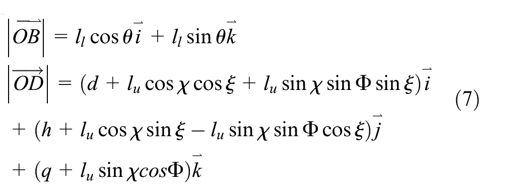
The position vector of the wheel knuckle can be defined as:

The unit vector of the lower control arm can be defined as:

By formulas (10)–(13), a point position can be obtained when the
Analysis and calculation of vector
In order to calculate vector

The second constraint is that the length of the steering arm remains constant for each position of the mechanism, so there is:

among them,

The third constraint is that for each position of the mechanism, the steering arm vector and the steering knuckle vector are perpendicular to each other
In equation (17), it can get:

among them,

In equations (17)–(19), the unknown parameters


Vector transformation: (a) schematic diagram of wheel static surface position vector, (b) schematic diagram of Angle change of vector ek, and (c) schematic diagram of the rotation of wheel knuckle relative to ek.
In order to get the any position of the vector on the wheel knuckle, the rotation matrix can be used and take the following steps: starting from the initial position of the steering arm, determine the rotation matrix of the unit vector of the steering arm from


The second rotation analysis requires a complete analysis of the rotation of wheel knuckle with respect to the unit vector

The matrix with a rotation angle of

Because of the related rotation matrix has obtained, the unit vector

Calculation of wheel alignment angle
In order to analysis and calculate the wheel alignment angle of the double wishbone suspension, the double wishbone suspension is simplified to obtain a schematic diagram as shown in Figure 7. The camber angle, caster angle, kingpin angle, and toe angle in Figure 7 can all be calculated by vectors. 12

Schematic diagram of wheel alignment angle of double wishbone suspension.
In Figure 7,

The camber angle shown in Figure 7 can be calculated by vectors

The caster angle shown in Figure 7 can be calculated by vectors

among them,

The kingpin angle of the suspension system can be calculated by vector
among them,

After analyzing the influence of the suspension motion on the wheel alignment angle, the opposite travel simulation on the front suspension and the rear suspension was carried out, the changes of toe angle and camber angle with wheel travel as shown in Figures 8 and 9 were obtained.

Variation diagram of toe angle with wheel travel.
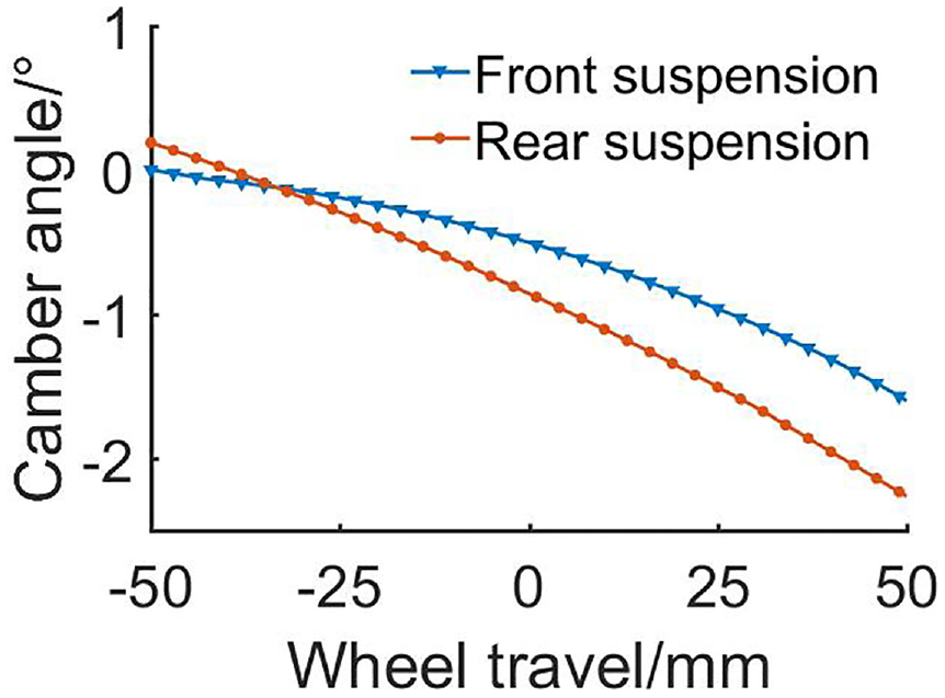
Variation diagram of camber angle with wheel travel.
In Figure 8, during the wheel travel downward, the toe angle of the front suspension wheel (the inner wheel when turning) increases in the positive direction, and the toe angle of the rear suspension wheel (the inner wheel when turning) increases in the negative direction. The toe angle of the corresponding outer wheel of the front suspension increases negatively, and the toe angle of the outer wheel of the rear suspension increases positively. For the front suspension, the toe angle of the inner wheel increases positively, and the toe angle of the outer wheel increases negatively, which will increase the understeer characteristics of the vehicle. For the rear suspension, the toe angle of the inner wheel increases negatively, and the toe angle of the outer wheel increases positively, which will also increase the understeer characteristics of the vehicle.
In Figure 9, when the wheel travels downward, the camber angle of the front and rear suspension wheel (the inner wheel when turning) increases in the positive direction. When the wheel travels upward, the camber angle of the wheel (the outer wheel when turning) of the front suspension and the rear suspension both increases in the negative camber direction. In terms of adhesion, the front suspension’s and the rear suspension’s outer wheel camber angle increase in the negative camber direction, the tire’s adhesion will be improved. For the perspective of understeer characteristics of the vehicle, when the vehicle is turning, the camber angle of the front suspension’s outer wheel increases to the negative camber direction, the understeer characteristic of the vehicle will decrease, and the camber angle of the rear suspension’s outer wheel increases to the negative camber direction, the understeer characteristics of the vehicle will increase.
Statics analysis of double wishbone suspension
When the wheels of the double wishbone suspension are excited by the road and jump, the hinge point of the suspension link and the link rod will move with the travel of the wheel, so the position of each hinge point will change accordingly. Through the theory of coordinate transformation, after selecting a reference point, the coordinates of other hinge points can be calculated accordingly. The force balance and torque balance equations can be used to calculate the force of the vehicle suspension hinge points and bushing.
Displacement analysis of double wishbone suspension’s connecting point
The schematic diagram of the double wishbone suspension is shown in Figure 10. In order to analysis the force and moment of suspension’s ball joint and bushing, firstly, the position transformation of each connection point of the double wishbone suspension is analyzed. 13 The double wishbone suspension is composed of upper control arm, lower control arm, wheel knuckle, springs, shock absorbers and tie rods. The four bushes A1 and A2, A3 and A4 in Figure 10 connect the upper and lower control arms to the vehicle body respectively. The ball joint D and the ball joint G respectively connect the wheel knuckle with the upper and lower control arms. The two ends of the coil spring and the shock absorber are installed between the lower control arm and the vehicle’s body, which are installed between the ball joints C and E, respectively.

Schematic diagram of double wishbone suspension system.
If an object rotates from one position to another without displacement, the coordinates of the object in the global coordinate system


When the rigid body rotates and moves at the same time, select point
The

In the same way, taking point


Calculate the forces and moments acting on the bushing
If a static external force

Superscript


The upper control arm is in a balanced state under the action of the reaction force and the reaction moment of the bushing, the spring, and the ball joint of the wheel knuckle. Therefore, the sum of each force component of all forces, as well as the sum of each force and each moment component of the connection point D in the global coordinate system is zero. According to this principle, the static balance equation of the upper control arm can be obtained and expressed as:


Take the lateral force in the interval

The force in the x direction of the rubber bushing.

The moment of the rubber bushing around the x-axis.
Statics analysis of multi-link suspension
When an external load acts on the contact point between the tire and the ground, the wheels, wheel knuckle and connection rods will move to new position due to the elastic deformation of the bushes and springs in the suspension. In this way, a new static equilibrium is reached. The new position of each bush in this load can then be calculated.
Displacement analysis of multi-link suspension’s connection point
The schematic diagram of the multi-link suspension is shown in Figure 13.

Schematic diagram of multi-link suspension.
For the wheel knuckle, when point
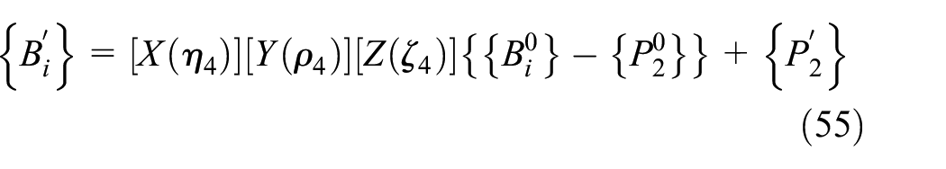
For connection rod
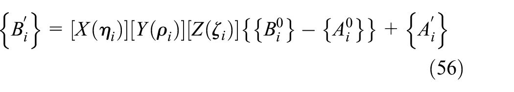
Where
According to equations (55) and (56), when external force acts on the suspension, the new position and displacement of each bush can be obtained.
Calculate the forces and moments acting on the rubber bushing
When an external force is applied to the wheel knuckle, the bushing will rotate and translate.
15
For the bushing

The superscript


Mark the forces and moments on the hinge points
Force balance and moment balance analysis
Under the action of the reaction force and moment of the hinge point

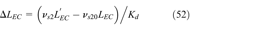
The initial length, deformed length and displacement of the spring satisfy the following formula:

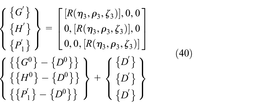
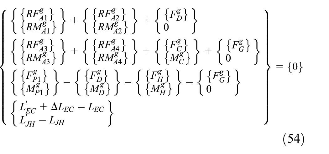
On the basis of the above analysis, the balance equations of the suspension system can be obtained. By combining the balance equation of the wheel knuckle (equation (61)), the balance equation of the rod (equation (62) and the constraint equation of spring (equation (63)), the equation of the multi-link suspension is expressed as:

Figure 14 shows the change of the force on the rear multi-link suspension bushing with the lateral force on the wheels. Figure 15 shows the change of the torque on the rear multi-link suspension bushing with the lateral force on the wheels.

The change of the bush’s force in the x-direction with the lateral force of the wheel.

The torque of the bushing around the x-axis changes with the lateral force of the wheel.
Analysis of the influence of suspension kinematics and compliance characteristic on vehicle dynamics
The actual deformation of the rubber bush during the movement of the suspension is more complicated, including the axial movement of the inner ring (metal inner surface) relative to the outer ring (metal outer surface), the movement of the inner and outer rings in different radial directions, and the rotation of the inner and outer rings around the axis etc. The suspension kinematics characteristic is the change characteristic of the wheel alignment angles caused by the geometric movement of the suspension. The kinematics characteristic of the suspension include wheel bouncing in the same direction and opposite direction. The kinematics characteristics of the suspension are analyzed in Figures 8 and 9. The characteristic of the tire force and the change of the wheel alignment angle caused by the deformation of the elastic elements such as the bushing in the suspension is called the compliance characteristic of the suspension. The compliance characteristic of the suspension includes the characteristic of the tires subjected the same direction lateral force, reverse lateral force, longitudinal force, same direction align torque, and reverse align torque. The impact of the bushing on the dynamic characteristic of the vehicle is mainly in two aspects, one is that due to the deformation of the bushing, when the tire is subjected to lateral force, longitudinal force and align torque, it will cause the wheel to produce additional steering angle, which will affect the steering characteristic of the vehicle. At the same time, the bushing will affect the force on the vehicle wheels, that is, it affects the dynamic characteristic of the vehicle by influencing the tire force.
The influence of suspension motion and bushing on the change of toe Angle and camber Angle
From the analysis of the front two parts, it can be seen that the force of the vehicle wheel will cause the deformation of the suspension bushing, and the deformation of the bushing will cause the change of the wheel alignment angle. Based on the force analysis about front double wishbone suspension and the rear multi-link suspension, the compliance characteristic simulation analysis of the double wishbone suspension and the rear multi-link suspension of the vehicle is carried out, the changes of the toe angle and the camber angle of the wheel with the lateral force and the longitudinal force as shown in Figures 16 to 19 are obtained.

The toe angle and camber angle of the front double wishbone suspension vary with the lateral force of the wheel.
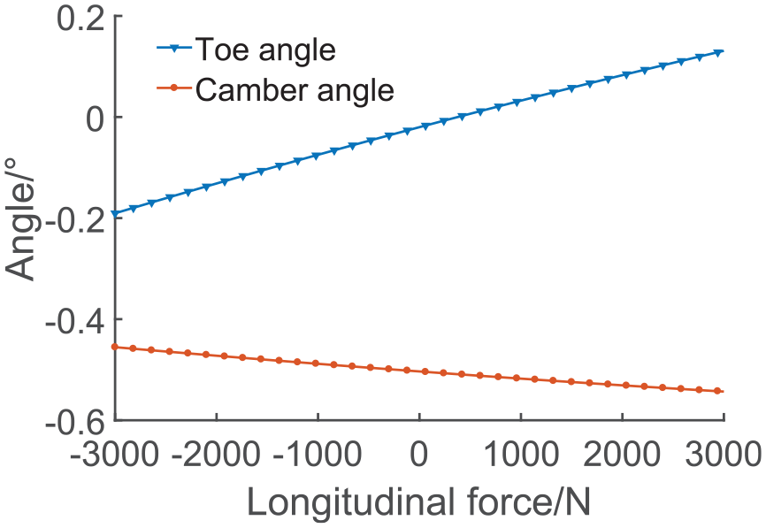
The toe angle and camber angle of the front double wishbone suspension vary with the longitudinal force of the wheel.

Changes in toe angle and camber angle of rear multi-link suspension with wheel’s lateral force.

Changes in toe angle and camber angle of rear multi-link suspension with wheel’s longitudinal force.
Figure 16 shows the change of toe angle and camber angle of the front double wishbone suspension with the lateral force of the wheel. In Figure 16, both the toe angle and the camber angle increase in the positive direction as the reverse lateral force increases. The toe angle and camber angle both increase in the negative direction as the positive lateral force increases. Figure 17 shows the change of toe angle and camber angle of the front double wishbone suspension with the longitudinal force of the wheel. In Figure 17, when the longitudinal force received by the wheels is the braking force, the toe angle increases in the negative direction with the increase of the braking force, and the camber angle increases in the positive direction with the increase of the braking force. When the longitudinal force received by the wheels is the driving force, the toe angle increases in the positive direction as the driving force increases, and the camber angle decreases in the negative direction as the driving force increases.
Figure 18 shows the change of the toe angle and camber angle of the rear multi-link suspension with the lateral force received by the wheels. In Figure 18, when the lateral force received is the reverse lateral force, the toe angle of the wheels changes less, and the camber angle increases in the positive direction as the reverse lateral force increases. When the lateral force received by the vehicle is a positive lateral force, the toe angle of the wheels changes less, and the camber angle increases in the negative direction. Figure 19 shows the change of the toe angle and camber angle of the rear multi-link suspension wheels when subjected to longitudinal force. In Figure 19, whether the wheel receives the driving force or the braking force, the toe angle changes little. For the camber angle, when the wheel receives the braking force, the camber angle increases in the negative direction, when the wheel receives the driving force, the camber angle of the wheel increases in the positive direction.
Effect of toe angle change caused by suspension movement and bushing deformation on tire side slip stiffness
When there is toe angle of the wheel, the side slip angle of the outer wheel is

The effect of toe angle on wheel’s side slip angle.
The average side slip stiffness of the inner and outer wheels is denoted as

The toe angle of the wheel itself and the change of the toe angle will affect the tire side slip angle. The change of the wheel’s toe angle caused by the wheel lateral force, longitudinal force and align torque is expressed as

For the toe angle, when designing the suspension, it requires to increase the side slip angle of the wheel during the change of the toe angle of the front axle caused by the deformation of the bushing, the toe angle of the rear axle wheels requires to reduce the wheel’s side slip angle during the change of the toe angle of the rear axle, so that the vehicle tends to understeer.
The effect of suspension motion and the change of camber caused by bushing on vehicle’s steering characteristic
The variation characteristics of wheel’s side slip Angle with relative centripetal acceleration are shown in Figure 21. When the camber is positive, the side slip angle is greater than when there is no camber, and when the camber is negative, it is smaller than when there is no camber. The understeer/oversteer trend of the vehicle will be affected by changes in camber as the function of centripetal acceleration (or the function of roll or the function of lateral force). When the centripetal acceleration is low, the front wheel’s camber changes in positive direction/rear wheel no change, or front wheel’s camber no change/rear wheel’s camber change in negative direction, the understeer tendency of the vehicle will increase; otherwise, the understeer will decrease. When the lateral acceleration is high, the front wheels have negative camber/the rear wheels have no camber, there is a slight oversteer of the vehicle; while the front wheels without camber/the rear wheels have a positive camber, there is a strong oversteer characteristic of the vehicle.

Effect of camber on understeer/oversteer characteristic.
The camber of the wheel will have an effect on the side slip angle of the wheel. The change of camber angle caused by the lateral force, longitudinal force and the align torque of the wheel is expressed as

When designing the suspension, for the wheel’s camber angle, when the centripetal acceleration is low, the deformation of the bushing is required to make the front wheel camber change in positive direction/rear wheel no change, or front wheel camber no change/rear wheel’s camber changes in negative direction, which will increase the understeer tendency of the vehicle. When the lateral acceleration is high, let the front wheels have negative camber/the rear wheels have no camber, so that the vehicle has a slight oversteer to avoid strong oversteer characteristic.
Lateral force on vehicle’s tires
During the vehicle’s movement, the lateral force received by a vehicle’s tire can be calculated by two parts, one is the product of the tire’s side slip stiffness and the cornering angle, and the other is the product of the lateral camber thrust coefficient and the camber angle. The side slip angle and camber angle of the tire are obtained by the suspension movement and suspension bushing deformation. The force obtained by the product of the tire side slip stiffness and the tire side slip angle is:
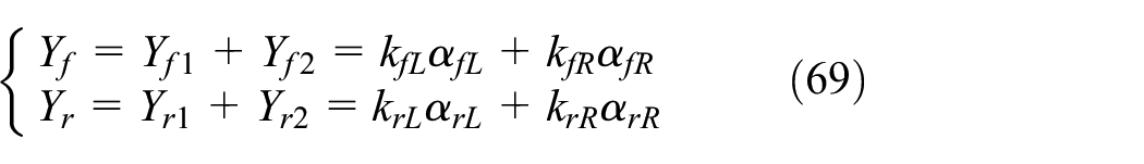
The lateral force obtained by product of the tire’s lateral thrust coefficient and the camber angle is:
The total lateral force produced by the suspension movement and the bushing’s deformation is:

Multi-objective optimization of vehicle’s handling stability
There are multiple evaluation parameters for the transient characteristics of vehicle. In order to explain these evaluation parameters in the form of formulas, the three degree of freedom vehicle dynamics model is used. Since there are multiple optimization targets and multiple optimization variables in the optimization, therefore, optimizing the bushing of the suspension based on the sine swept input to improve the transient dynamics of the vehicle requires multi-objective optimization. Therefore, on the basis of the three degree of freedom vehicle’s dynamics, the optimization targets of vehicle’s transient characteristic are derived, the multi-objective optimization program are established.
Optimize objective function
For parameter-oriented vehicle’s dynamics models, the three degree of freedom vehicle dynamics model is mostly used at present, because the three degrees of freedom vehicle’s dynamic model is simpler than other dynamic models, but it can describe the main motion characteristic and force characteristic of the vehicle. The vehicle’s three degree of freedom model considers the vehicle’s lateral, yaw and roll these three degrees of freedom. For the transient characteristic of the vehicle, the three degree of freedom vehicle dynamics model is also easy to describe the frequency characteristic. The main parameters such as gain and delay time can also be derived with the help of the three degree of freedom vehicle dynamics model. Because the sine swept steering input simulation is used in this article, the vehicle’s roll, lateral and yaw these three degrees of freedom are also mainly considered. The three degree of freedom vehicle dynamics model is:

After Laplace transform of equation (72), the characteristic equation is:

Based on the formula (73), the objective function based on the sine swept steering input simulation is:
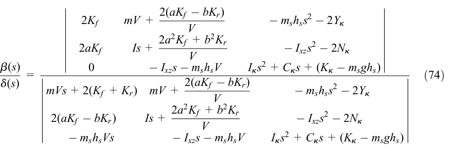


In equations (74)–(76),

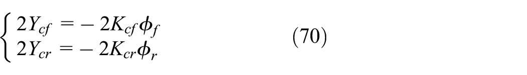
In equation (72), the side slip stiffness
In equations (74)–(76), make

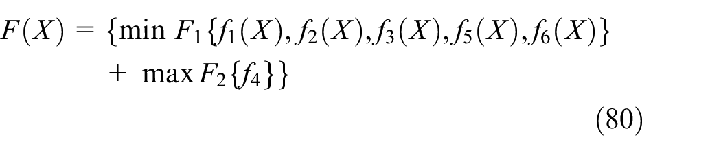
The overall optimization objective functions are:

Sensitivity analysis of the influence of suspension bushing’s stiffness on vehicle handling stability
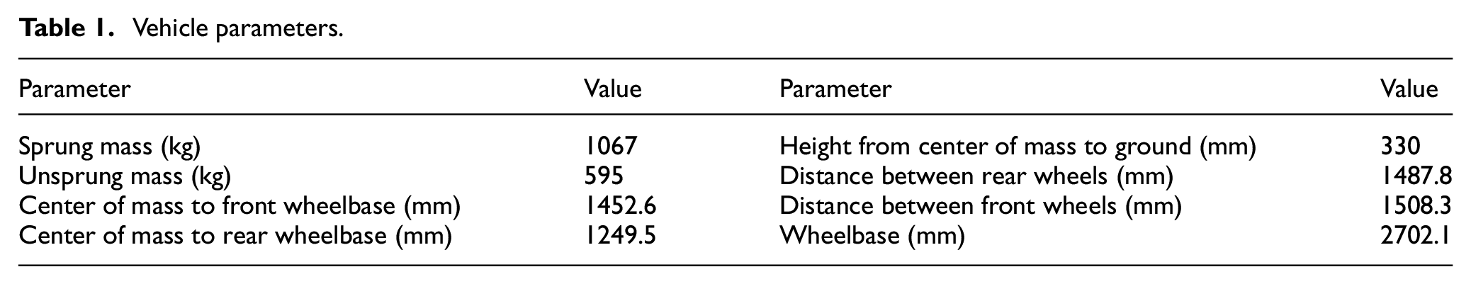
The vehicle’s parameters used in the optimization are shown in Table 1:
Vehicle parameters.
There are eight bushings connecting the connection rods and the vehicle body in Figures 10 and 13, four for the front suspension and four for the rear suspension, and each bushing has stiffness in six directions. Taking the upper rear control arm on the front suspension as an example, the bushing is named
There are eight bushings in Figures 10 and 12, so there are 48 stiffness values, but some stiffness values have little effect on the handling stability of the vehicle, and some stiffness values have a greater influence on the handling stability of the vehicle. In order to find out the bushing stiffness values that have a greater impact on the handling stability of the vehicle, the sensitivity analysis of these 48 stiffness values is carried out first, and then several stiffness values with higher sensitivity are selected for optimization analysis. After the sensitivity analysis, five stiffness values with greater sensitivity are selected as shown in Table 2.
Bushing stiffness with larger sensitivity value.

Optimization algorithm
By optimizing the stiffness of the suspension bushing to improve the handling stability of the vehicle, the multi-objective optimization method and algorithm are adopted. The NSGA-II algorithm is a relatively successful algorithm used in multi-objective optimization algorithms. 16 In non-dominated sorting, individuals close to the Pareto frontier are selected, which enhances Pareto’s forward ability. Combined with the analysis of section 7.2, the mathematical expression of multi-objective optimization is as follows:

The mutation operation in generating sub-individuals according to the SBX method is:


At present, the optimization objective function used in the optimization of vehicle handling stability is mainly realized by vehicle dynamic parameter modeling. In the process of establishing parameter model, some secondary factors and degrees of freedom of the vehicle are often ignored, which leads to the optimized model compared with the actual vehicle, the error is larger. In order to make the vehicle’s model as close as possible to the real vehicle model, this paper adopts the multi-body dynamics model, that is, the multi-objective optimization of vehicle’s handling stability is carried out for the multi-body dynamics model.
Since the sine swept steering input test is used in this paper to evaluate the handling stability of a vehicle, the parameters of the sine swept steering input simulation to evaluate the vehicle’s handling stability are taken as the optimization objectives, and the suspension bushing stiffness with higher sensitivity are taken as the optimization variables to perform multi objective optimization. After the multi objective optimization of the whole vehicle, the optimization iterative diagram of the optimization targets is shown in Figures 22 to 27.

Iterative diagram of the maximum gain value of the yaw rate relative to the steering wheel angle.
Iterative graph of yaw rate gain at 0.5 Hz relative to the steering wheel angle.

Iterative diagram of resonance frequency.
Iteration diagram of roll angle gain relative to the lateral acceleration.

Iterative diagram of lateral acceleration delay time.
Iterative diagram of yaw rate delay time.
Figures 22 and 23 are iterative graphs of yaw rate gain with the steering wheel angle. Figure 22 is the maximum value of the yaw rate gain relative to the steering wheel angle, and Figure 23 is the yaw rate gain value at 0.5 Hz relative to the steering wheel angle. In the performance of the frequency characteristics of the vehicle, the smaller the maximum gain value of the yaw rate relative to the steering wheel angle, the more stable the vehicle. Therefore, it is hoped that the maximum gain value of the yaw rate relative to the steering wheel angle will be minimized during optimization. The change trend of the iterative graphs in Figures 22 and 23 meets the requirements of the optimization goal.
Figure 24 is an iterative diagram of the resonance frequency. The larger the resonance frequency, the more stable the vehicle. The resonance frequency in Figure 24 is continuously increasing as the optimization progresses, which meets the requirements of the optimization goal. Figure 25 shows the roll angle gain relative to the lateral acceleration. In Figure 25, the roll angle gain relative to the lateral acceleration is increased compared to the original vehicle, but the increased value is small, so it has little effect on the handling stability of the vehicle.
Figures 26 and 27 show the delay time of lateral acceleration relative to the steering wheel angle and the delay time of yaw rate relative to lateral acceleration. The smaller the delay time, the faster the response of the vehicle. Figures 26 and 27 reflect that the delay time is decreasing, which is beneficial to improve the response speed of the vehicle, indicating that the optimization is carried out in accordance with the required target.
Optimization results
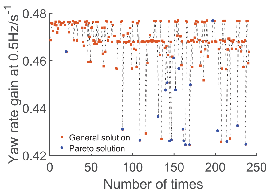
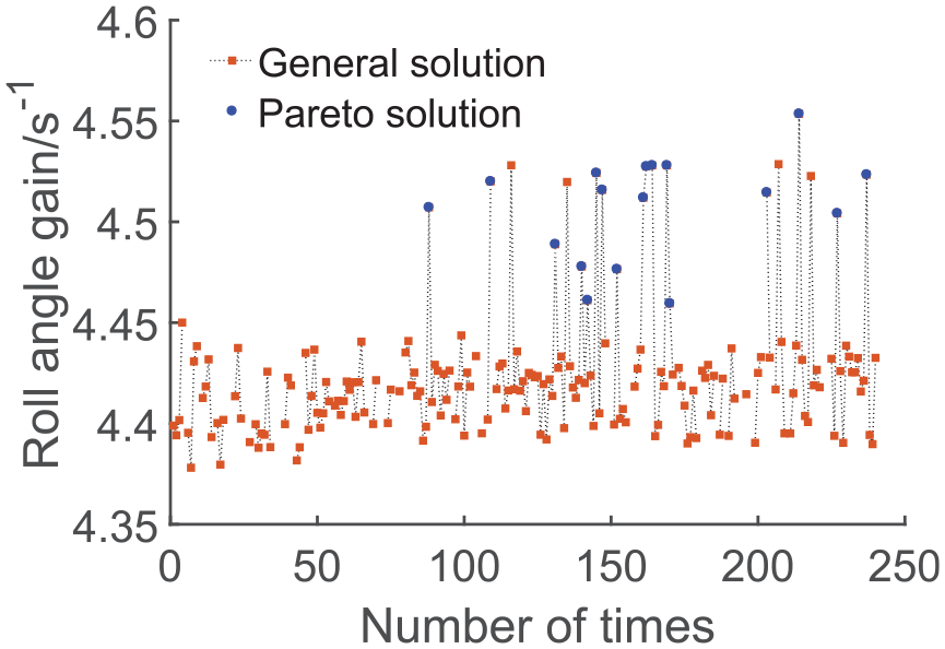
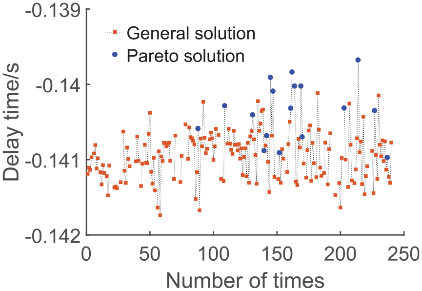
After the multi-objective optimization for the transient characteristic of the vehicle, the corresponding Pareto solution sets are obtained, as shown in Figures 28 to 33. Among them, the black point represents the general solution, the blue point represents the Pareto solution, and the green point represents the relatively optimal solution. Delay time 1 refers to the delay time of the lateral acceleration relatives to the steering wheel angle, and delay time 2 refers to the delay time of yaw rate relatives to the lateral acceleration.

Pareto solution sets of yaw rate gain at 0.5 Hz with resonance frequency.

Pareto solution sets of roll angle gain at 0.5 Hz relative to yaw rate gain at 0.5 Hz.

Pareto solution sets of delay time 1 with yaw rate gain at 0.5 Hz.
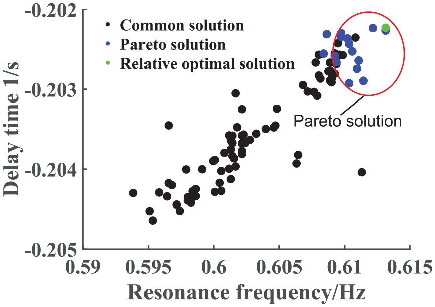
Pareto solution sets of delay time 1 relative to resonance frequency.

Pareto solution sets of delay time 1 relative to delay time 2.

Pareto solution sets of delay time 2 relative to yaw rate gain.
Through optimization analysis, Pareto solution sets and relative optimal solution are finally obtained. The comparison of parameters before and after optimization of the vehicle are shown in Table 3.
Comparison of parameters before and after optimization.

Comparative analysis of optimization results of vehicle handling and stability
In order to analysis the optimization effect, a Pareto solution is selected from the optimization results and compared with original vehicle. In order to ensure that the handling stability of the vehicle is optimized and improved, comparisons are made from two aspects of the vehicle’s transient characteristics and steady-state characteristics.
Comparative analysis of vehicle’s transient characteristics
Bring the selected Pareto solution into the original vehicle for simulation analysis, and compare the results with the original vehicle, the result comparison chart in Figures 34 to 39 are obtained. Figure 34 shows the yaw rate gain relative to the steering wheel angle. In Figure 34, in the range of 0 to 1 Hz, especially at 0.5 Hz, the curve of the optimized yaw rate gain relative to the steering wheel angle is smaller than that of the original vehicle, which meets the requirements of the optimization goal. When the frequency exceeds 1 Hz, the difference of the yaw rate gain before and after optimization is not obvious. Since the frequency of the driver in the process of driving the vehicle rarely exceeds the range of 1 Hz, the high frequency range is not considered.

Yaw rate gain relative to the steering wheel angle.

Delay time of yaw rate relatives to the lateral acceleration.

Roll angle gain relative to the lateral acceleration.

An enlarged view of roll angle gain relative to the lateral acceleration.

Delay time of lateral acceleration relative to the steering wheel angle.

The enlarged view of the lateral acceleration’s delay time relative to the steering wheel angle.
Figure 35 is the delay time of yaw rate relatives to the lateral acceleration. In Figure 35, at 0.5 Hz, the difference to the delay time of yaw rate between optimized and original vehicle is obvious, and it is reduced after optimization compared with the original vehicle, which meets the requirements of optimization goals. Between 0 and 1 Hz, the optimized delay time of yaw rate is basically smaller than the original vehicle. When the frequency exceeds 1 Hz, the difference of yaw rate delay time between the optimized vehicle and the original vehicle is small. Since the frequency rarely reaches above 1 Hz during the operation of the vehicle, the situation above 1 Hz will not be discussed too much.
Figure 36 shows the roll angle gain relative to the lateral acceleration. In Figure 36, from low frequency to high frequency, as the frequency increases, the difference of roll angle gain between the optimized vehicle and original vehicle is relatively small. After enlarging the curve at 0.5 Hz, the situation shown in Figure 37 is obtained. In Figure 37, the roll angle gain relative to the lateral acceleration after optimization is increased than original vehicle, but the increased value is relatively small and within an acceptable range. Because it is a multi-objective optimization, it is normal for individual optimization objectives to fail to reach the optimum.
Figure 38 shows the delay time of the lateral acceleration relative to the steering wheel angle, and after enlarging the range around 0.5 Hz in Figure 38, the delay time of the lateral acceleration around 0.5 Hz relative to the steering wheel angle as shown in Figure 39 is obtained.
In Figures 38 and 39, the absolute value of the lateral acceleration’s delay time of the optimized vehicle is reduced, but in general, the difference of the lateral acceleration’s delay time between the optimized vehicle and original vehicle in the entire frequency range is smaller. Because it is a multi-objective optimization, it is difficult to achieve all the optimization objectives to reach the optimal state, the lateral acceleration’s delay time after optimizing didn’t significantly reduced but it is acceptable.
Comparison and analysis of steady state with constant radius cornering simulation
In order to further verify the improvement of the vehicle’s dynamics characteristics after the vehicle optimization, the constant radius cornering simulation of the whole vehicle before and after the optimization is compared and analyzed. The curve of the steering wheel angle with the lateral acceleration shown in Figure 40 and the curve of the roll angle with the lateral acceleration shown in Figure 41 are obtained.

The curve of steering wheel angle with the lateral acceleration.

The curve of roll angle with the lateral acceleration.
In Figure 40, at the same lateral acceleration, the steering wheel angle of the optimized vehicle is larger, indicating that the understeer characteristic of the vehicle is increased, and the vehicle tends to be more stable. In Figure 41, under the same lateral acceleration, the optimized vehicle’s roll angle has increased, but the increase value is not much and within in the acceptable range.
Conclusion
The stiffness calculation of vehicle suspension bushing is analyzed and the multi-body dynamic model of vehicle’s front and rear suspension is established according to the actual vehicle. The influence mechanism of the bushing on the suspension wheel alignment angle and the suspension force is analyzed in detail and systematically. Through sensitivity analysis, five bushes that have a greater impact on the transient characteristics of the vehicle are selected, and multi-objective optimization is performed for the selected bushings. The specific conclusions obtained are:
Through the calculation of the vector, the link position and link angle during the movement of the double wishbone suspension are analyzed in detail, and the wheel alignment angle of the double wishbone suspension is finally calculated. Through the simulation calculation of the multi-body dynamics model, the toe angle and camber angle change with the wheel travel are obtained.
The bushing deformation and bushing force of double wishbone suspension and multi-link suspension are analyzed, and the relationship between bushing deformation and suspension compliance characteristics is explained.
Sensitivity analysis shows that for the double wishbone suspension, the torsional stiffness of the lower front control arm bushing around the z axis, the translational stiffness of the lower rear control arm bushing along the y direction, and the translational stiffness of upper front control arm bushing along the z direction have a greater impact on the vehicle’s transient characteristic. For the rear multi-link suspension, the stiffness of the lower front control arm bushing along the z direction and the torsional stiffness of the lower rear control arm bushing around the z-axis have a greater impact on the vehicle’s transient characteristics.
For the front suspension, when the torsional stiffness of the lower front control arm bushing around the z axis increases by 31%, the translational stiffness of the lower rear control arm bushing along the y direction is reduced by 99.9%, and the translational stiffness of the upper front control arm bushing in the z direction is reduced by 97%. For the rear suspension, when the stiffness of the lower front control arm bushing along the z direction is reduced by 82% and the torsional stiffness of the lower rear control arm bushing around the z axis is reduced by 79%, the yaw rate gain at 0.5 Hz is reduced by 6.4%, and the roll angle gain is increased by 2.7%, the delay time of yaw rate is reduced by 15%, the delay time of roll angle is unchanged, and the resonance frequency is increased by 31.7%. From the perspective of steady-state conditions, the understeer trend of the vehicle increases, and the roll angle increases slightly, but it is within an acceptable range.
Footnotes
Appendix
Handling Editor: James Baldwin
Declaration of conflicting interests
The author(s) declared no potential conflicts of interest with respect to the research, authorship, and/or publication of this article.
Funding
The author(s) disclosed receipt of the following financial support for the research, authorship, and/or publication of this article: This project was supported by National Natural Science Foundation of China (NSFC) (No.51965026), Yunnan Province Applied Basic Research Foundation (No. 2018FB097) and Scientific Research Fund Project of Yunnan Provincial Education Department (No. 2018JS022). The authors are greatly appreciated for the financial support.