Sage Journals: Discover world-class research

Abstract

In order to realize the active and compliant motion of the robot, it is necessary to eliminate the impact caused by processing contact. A hybrid control strategy for grinding and polishing robot is proposed based on adaptive impedance control. Firstly, an electrically driven linear end effector is designed for the robot system. The macro and micro motions control model of the robot is established, by using impedance control method, which based on the contact model of the robot system and the environment. Secondly, the active compliance method is adopted to establish adaptive force control and position tracking control strategies under impact conditions. Finally, the algorithm is verified by Simulink simulation and experiment. The simulation results are as follows: The position tracking error does not exceed 0.009 m, and the steady-state error of the force is less than 1 N. The experimental results show that the motion curve coincides with the surface morphology of the workpiece, and the contact force is stable at 10 ± 3 N. The algorithm can realize more accurate position tracking and force tracking, and provide a reference for the grinding and polishing robot to realize surface processing.

Keywords

Grinding and polishing robot force and position hybrid control adaptive impedance control

Introduction

With the development of large fan blades, aircraft turbine blades, and propellers, the surface quality requirements of complex curved workpieces are constantly increasing, and the machining process requires higher precision. The grinding and polishing process requires high precision. However, the current manual grinding and polishing operation is inefficient, time-consuming, and processing accuracy cannot be guaranteed. In addition, the polishing operation environment is noisy and dusty, which can easily cause occupational diseases and even personal injury.¹ Industrial robots have the advantages of low price, large working space, and strong flexibility. In order to solve the shortcomings of manual polishing and the advantages of applying industrial robots, the development of grinding and polishing robot systems and other types of automatic polishing equipment has received extensive attention.² Grinding and polishing are typical contact processing, which is different from non-contact operations such as spraying. The contact between the end effector and the surface of the workpiece will generate force, which affects the contact stress between the polishing tool and the workpiece. The contact stress has an important influence on the surface quality of the workpiece.³ When it is too large, it will cause a large amount of removal, but when it is too small, it will reduce the grinding and polishing efficiency.⁴ Therefore, the constant force and compliant motion control of the grinding and polishing robot have become the main research direction to improve the quality of grinding and polishing.

The compliant control method can be roughly divided into two categories: direct method and indirect method. The direct method refers to the direct control of force and motion respectively, while the indirect method refers to the control of the dynamic relationship between force and motion to achieve compliant motion. The most representative way to directly control motion and force is the force/position hybrid control method proposed by Raibert and Craig.⁵ This method uses the orthogonal and complementary characteristics of the robot position subspace and the force subspace during interaction to perform decoupling control of force and position.⁶ It is mainly used in fields where precise force control is required. The prerequisite for its application is that the force and position trajectories required for the contact process are known, and it is not suitable for interactive collaboration in an unstructured environment. The indirect method controls the relationship between the external force and the motion state of the robot, satisfies the characteristics of the compliant motion, and realizes the compliant control of the robot. Common methods include impedance control,⁷ admittance control⁸ and stiffness control.⁹

The method proposed by Hogan¹⁰ to realize the compliant motion control of the robot based on the indirect method is called impedance control. Impedance control can ensure that the robot moves in a constrained environment and maintains appropriate interaction forces. It has strong robustness to some uncertain factors and external interference, and has less calculation amount in application. It is widely used in the compliant motion control of robots. However, there are still many difficulties in impedance control. On the one hand, the kinematics and dynamics of the robot itself have time-varying, strong coupling and nonlinear characteristics, and only using impedance control cannot solve the problems in engineering applications.¹¹ On the other hand, impedance control has disadvantages such as poor trajectory tracking ability, and the expectation force cannot be accurately controlled.¹² Therefore, in the practical application of impedance control, the traditional structure should be changed or integrated with other control methods. For example, impedance control is combined with adaptive control, fuzzy control, neural network and learning control.¹³

In order to realize robot constant force processing, there are currently two methods for using robots to perform active and compliant motion of processing tools through force feedback: straight arm system and arm-around system. In the straight arm robot system, the contact stress is controlled by the constrained motion of each joint. Because of the large size and weight of the robot, the dynamic response is usually slow in the control process. At the same time, the large inertia of the robot will have a great impact on the tool and the workpiece, and it is easy to damage the tool or the workpiece. Therefore, the system becomes unstable under high bandwidth.¹⁴ However, the grinding and polishing process requires dynamic high-frequency adjustment of the contact stress to adapt to sudden changes in the surface curvature of the workpiece. The arm-around system realizes contact stress control by externally adding active end effector movement, which is the most commonly used method in active compliance movement. This is also called the macro-micro robot system method. Industrial robots are called macro robots, which mainly provide surface path tracking of workpieces, and end effectors are called micro robots, which realize tool posture and contact force adjustment.⁴ Compared with the straight arm system, the active compliance method of the macro-micro robot system can effectively adapt to the high bandwidth and high precision requirements in the processing operation.¹⁵

The research on using the macro-micro robot system for active compliant motion control to improve the performance of the robot mainly focuses on the structure design of the micro robot and its control method. Mohammad et al.¹⁶ proposed an active end effector, this design reduced the undesirable vibration in the automatic grinding and polishing process through the limited inertia effect. Tol et al.¹⁷ proposed a macro-micro robot system that integrates parallel kinematics (PKM) and 2-DOF micro-robots into an automatic deburring and finishing system, which improved the force control performance of the robot. The system relies on an accurate model of the workpiece geometry. Jamisola et al.¹⁸ proposed the use of a force/position hybrid control algorithm to realize the compliant motion of macro and micro robots. Since the algorithm is limited to the position and force control on the same axis, there will be problems when processing complex workpieces with large geometric errors. Duan et al.¹⁹ combined impedance control and force/position hybrid control to achieve the process of tracking the contour of the workpiece in an uncertain environment, but did not consider using active end effector to improve response speed.

The above algorithms have disadvantages such as poor adaptability for machining uncertain surface contours and slow response speed. A hybrid active compliant control strategy for grinding and polishing robots based on adaptive impedance control is proposed. It meets the requirements of high-bandwidth and high-precision machining of complex curved surfaces and reduces the impact caused by sudden changes in contact force. In the control strategy, the industrial robot performs macro position control, and the end effector switches between micro position control and force control. Force control adopts adaptive impedance control and force/position hybrid control method. Finally, the effectiveness of the algorithm is verified by the constant force active compliant motion control simulation.

System modeling

Structural design

The grinding and polishing robot system is a system that connects the end effector to the end of the industrial robot through series connection. The end effector is connected by the arm-around method to realize the contact stress control during the grinding and polishing process. The structure of the grinding and polishing robot is shown in Figure 1. The six-degree-of-freedom industrial robot in the figure is used as a macro robot, and the end effector driven by a voice coil motor is used as a micro robot. The system has the characteristics of large working space, fast response speed and high precision.

Figure 1.

Structure diagram of grinding and polishing robot.

Figure 2 is a structural diagram of the end effector. The end effector includes a connecting flange, a voice coil motor module, a mounting flange, a force sensor and a polishing module. The voice coil motor module includes a linear voice coil motor, a linear guide and a bracket. The polishing module includes electric spindle or high-speed motor, tool holder and grinding head. In the voice coil motor module, the linear voice coil motor is composed of a stator and a mover. The stator is fixedly connected to the end of the industrial robot through a connecting flange to ensure a rigid connection of the linear voice coil motor during operation. On the linear guide rail, the mover moves along the axial direction in the stator to prevent the coil from deflection around the axis. The grating displacement sensor detects the mover position in real time. The voice coil motor module and the grinding module are connected through a force sensor, which is used to detect the torque and grinding force of the grinding module in real time. The polishing module provides the rotating movement of the grinding head through the electric spindle, and the designed tool holder is used to facilitate the replacement of the grinding head.

Figure 2.

End effector structure diagram.

In the grinding and polishing robot system, the industrial robot is used for coarse adjustment of the macro position. The end effector processes the displacement sensor signal and the force sensor signal through the controller to form a dual-loop control of the force position, thereby realizing fine position adjustment. The position control loop is controlled by the displacement sensor to control the stroke and position accuracy. The force control loop feeds back the contact force signal to the controller, and converts it into a position signal through the controller. The force sensor measures the actual contact force signal of the polishing module and converts it into the driving signal of the voice coil motor module and the posture adjustment signal of the industrial robot. It is used for real-time adjustment of the end effector to realize the closed-loop control of the contact stress of the workpiece.

The traditional design uses the electric motor as the power source and transmits the grinding force through shafts, gears and other components. In this design, a voice coil motor is used to provide driving force for the end effector and an electric spindle is used to provide grinding force. This reduces the load required for the motion state while satisfying the robot polishing process. The scheme using the motor and the shaft has a relatively high load. On the one hand, the end effector needs to output more force, which will increase the weight of the end effector and require high-load industrial robots. On the other hand, the movement of the motor and the shaft may cause high noise and high vibration of the end effector, which will reduce the control performance. In addition, the electric spindle can output force to meet the grinding requirements under the light weight condition, which reduces the overall quality of the end effector. Therefore, the weight of the end effector can be reduced by using a voice coil motor and an electric spindle. This design realizes the horizontal or vertical installation of the electric spindle by changing the clamping method of the tool holder. In this way, the overall size of the end effector can be adjusted, the working range of the robot and the processing direction of the grinding and polishing head can be changed to meet the use of more occasions.

Robot macro motion control

As industrial robots have the characteristics of wide working range, fast movement speed and large displacement, the algorithm that controls the movement of the grinding and polishing robot system in a large range is called robot macro motion control. The industrial robot joint 1 to joint 3 and joint 4 to joint 6 consider the position motion process control and end effector posture control, respectively.

Industrial robot joints select speed closed loop for motion control. The RMRC (Resolved Motion Rate Control) algorithm is simple and easy to provide speed commands to industrial robot controllers, so it is chosen as the control algorithm of industrial robots.²⁰ The RMRC algorithm uses the robot kinematics differential to convert the joint speed into the end working space speed, which can be computed as follow:

\overset{\cdot}{x} = J (θ) \overset{\cdot}{θ}

(1)

where J(θ) is the Jacobian matrix; $\overset{\cdot}{x}$ is the task velocity vector; $\dot{θ}$ is the joint velocity vector. Find the inverse solution of equation (1) and obtain the value $\overset{\cdot}{θ}$ .

\overset{\cdot}{θ} = J^{+} (θ) \overset{\cdot}{x} + (I - J^{+} (θ) J (θ)) b

(2)

where J⁺(θ) is the pseudo-inverse matrix of the Jacobian matrix. For J (θ) is non square matrix, its inverse matrix is not defined. Moore-Penrose inverse matrix can guarantee the uniqueness of solution. Thereby, Moore-Penrose pseudo-inverse is used in (2). b is the zero-space vector of J; I is the identity matrix. Considering the multi-joint robot, the dynamic characteristics of the system can be described by the second-order nonlinear differential equation as:²¹

M (θ) \overset{\cdot\cdot}{θ} + C (θ, \overset{\cdot}{θ}) + τ_{fric} (\overset{\cdot}{θ}) + g (θ) = Γ_{macro}

(3)

Through the model of formula (3), taking $\overset{\cdot}{θ}$ in formula (2) as the control input of the system, the control law is

Γ_{macro} = k_{p} e_{m} + k_{d} {\overset{\cdot}{e}}_{m} + τ_{fric} (\overset{\cdot}{θ}) + g (θ)

(4)

e_{m} = θ_{r} - θ

(5)

where M(θ) is the positive definite inertia matrix; $C (θ, \overset{\cdot}{θ})$ is the Centrifugal force and Coriolis force; τ_fric(θ) is the friction vector; g(θ) is the gravity vector; θ_r and θ are the expected angular displacement of the joint and the actual joint angle displacement, respectively; e_m is the tracking error; k_p and k_d are the proportional and differential coefficients of PD control, respectively.

Robot micro motion control

The end effector has a small working space, but has the characteristics of fast response speed and high precision. The algorithm that controls the small-scale movement of the grinding and polishing robot system on the surface of the workpiece is called robot micro-motion control. This section mainly considers the position control of the end effector.

Because of the complexity of the robot dynamic model, it is considered to simplify the control algorithm design. Firstly, in the process of modeling and controlling the macro micro robot system, Zheng Ma considered that the operation process was low-speed motion and only considered gravity compensation.²² In the experiment, the moving speed of the robot is set at 6–20 mm/s, and the desired contact force control is achieved. Secondly, in the actual grinding and polishing process, the robot movement speed is 10–40 mm/s, which can obtain the desired processing quality. Finally, through the above, it is considered that the robot operation in this paper is mainly low-speed motion, which meets the requirements of the dynamic model to simplify the dynamic model by ignoring the speed and acceleration terms when the joint speed and acceleration are small. In the follow-up simulation and experiment, the other coefficients of dynamics are taken as 0 to simplify the model and design the control algorithm. There are two control algorithms for the end effector and the workpiece from no contact to a stable contact process:

PD control

In this paper, the robot operation is mainly low-speed motion, ignoring errors such as Coriolis force, and mainly studying gravity errors. In robot force control operations, the external force reading of the sensor is usually reset to zero for accuracy. When the robot is in an unloaded state, the sensor installed between the end effector of the robot and the workpiece does not read zero, so the end effector needs to be compensated for gravity. The influence of gravity is removed from the sensor reading, so that the compensated sensor reading is always zero when it is not affected by external forces. The position control method using PD with gravity compensation, the control law is:

Γ_{mi} = k_{pmi} e_{mi} + k_{dmi} \dot{e_{mi}} + g_{mi} (θ)

(6)

e_{mi} = θ_{rmi} - θ_{mi}

(7)

where g_mi(θ) is the n × 1 order gravity vector; θ_rmi and θ_mi are the n × 1 order end effector joint expected angle vector and joint angle vector; e_mi is the tracking error; k_p and k_d are the proportions and the differential coefficient of PD control, respectively. n is the number of end effector joints. In this article, the end effector has 1 degree of freedom, so the value of n is 1.

The force sensor on the end effector is connected to the polishing module. The force information collected by the sensor includes the weight information of the polishing module, and the force information needs to be processed to obtain the gravity compensation amount. The gravity direction of the grinding head is the negative direction of the Z-axis of the robot base coordinate system, and the corresponding gravity vector is set to $g_{o} = [\begin{matrix} 0 & 0 & G \end{matrix}]$ . When solving the grinding process g_mi(θ), the tool gravity vector needs to be projected to the robot end coordinate system.

During the grinding and polishing process of the robot, the end posture is constantly changing. Set the transformation matrix of the robot end as R. At the initial position of the robot, the three coordinate axis vectors of the force sensor information collection coordinate system are expressed as ${\vec{x}}_{0}$ , ${\vec{y}}_{0}$ , ${\vec{z}}_{0}$ . With the transformation process of the robot’s end posture, the direction vectors of the force information collection system’s coordinate axis under the base frame are $\vec{x}$ , $\vec{y}$ , $\vec{z}$ :

{\begin{matrix} \vec{x} = R \cdot \vec{x_{0}} \\ \vec{y} = R \cdot \vec{y_{0}} \\ \vec{z} = R \cdot \vec{z_{0}} \end{matrix}

(8)

The conversion matrix R_a from the base coordinate system to the force sensor information collection coordinate system is,

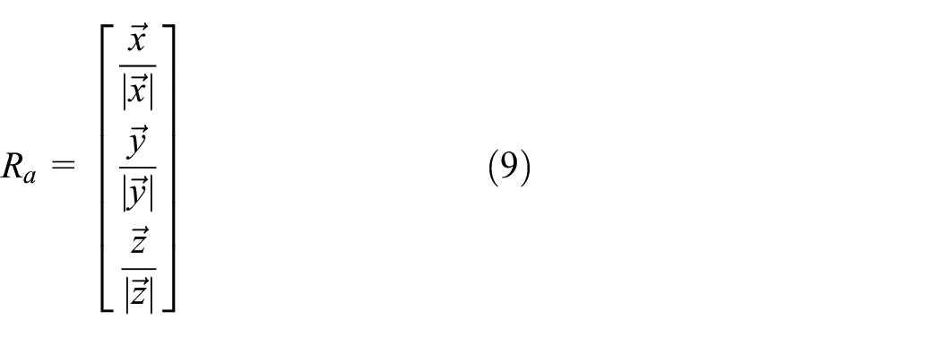
R_{a} = [\begin{matrix} \frac{\vec{x}}{| \vec{x} |} \\ \frac{\vec{y}}{| \vec{y} |} \\ \frac{\vec{z}}{| \vec{z} |} \end{matrix}]

(9)

The gravity vector $g_{o} = [\begin{matrix} 0 & 0 & G \end{matrix}]$ under the base frame is projected to the force sensor information collection frame.

g_{mi} (θ) = R_{a} \cdot \vec{g_{0}}

(10)

Adaptive impedance control

For the grinding and polishing process, the adaptive impedance control method is adopted for force control. The algorithm is as follows:

According to the definition of impedance control, it can be described as a second-order model:

{\begin{matrix} m Δ \overset{\cdot\cdot}{x} + b Δ \overset{\cdot}{x} + k Δ x = - e \\ Δ x = x - x_{r} \\ e = f_{e} - f_{r} \end{matrix}

(11)

where m, b, and k are the inertia, damping, and stiffness of the end effector; x and x_r are the actual position and the desired position; f_e and f_r are the actual contact force and the desired contact force.

Simplify the contact force model between the end effector and the workpiece to a spring model:

f_{e} = {\begin{matrix} k_{e} (x - x_{e}) x > x_{e} \\ 0 x < x_{e} \end{matrix}

(12)

where k_e is the environmental stiffness, and x_e is the environmental position.

The expected position in impedance control is a fixed value. When the actual contact position deviates from the expected position, a large contact force will appear, causing inaccurate position tracking. The following content will analyze the conditions of accurate position tracking in impedance control.

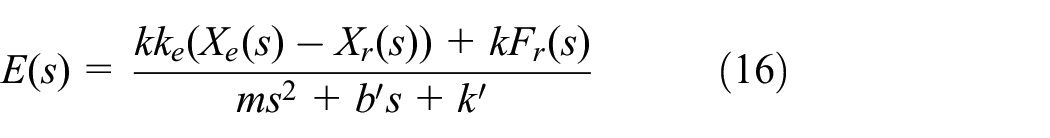
During the grinding and polishing process, the contact between the end effector and the workpiece will cause a sudden change or jitter of the axial force. Impedance control is not sensitive to changes in the end contact force, which makes it impossible to adjust the axial contact force more quickly. In order to improve the accuracy of the axial position tracking of the grinding and polishing robot, formula (11) can be rewritten as:

m \overset{\cdot\cdot}{x} + b \overset{\cdot}{x} + k (x - x_{r}) = - (k_{p} e + k_{d} \overset{\cdot}{e})

(13)

With the impedance model equation (11), the proportional-derivative control of the contact force is introduced. k_p and k_d are the coefficients corresponding to the contact force and the change speed of the contact force. Adjusting k_p can reduce the tracking error, and adjusting k_d can change the sensitivity of the model to changes in contact force, thereby improving the overall position tracking performance of the model. Due to the slow axial movement speed during the machining process, the desired position is regarded as a constant in the analysis.

From the environmental contact model equation (12), the actual position x can be expressed as:

x = \frac{f_{e}}{k_{e}} + x_{e} = \frac{1}{k_{e}} (f_{r} - e) + x_{e}

(14)

Substituting formula (14) into formula (13),

m \overset{\cdot\cdot}{e} + b' \overset{\cdot}{e} + k' e = k f_{r} + k k_{e} x_{e} - k k_{e} x_{r})

(15)

where, $b' = b - k_{d} k_{e}$ , $k' = k - k_{p} k_{e}$ .

Laplace transform on equation (12):

E (s) = \frac{k k_{e} (X_{e} (s) - X_{r} (s)) + k F_{r} (s)}{m s^{2} + b' s + k'}

(16)

when the expected force is constant, $F_{r} (s) = f_{r} / s$ , $X_{e} (s) = x_{e} / s$ . The steady-state error of contact force tracking is:

e_{ss} = lim_{s \to 0} sE (s) = lim_{s \to 0} \frac{k}{k'} [s k_{e} X_{r} (s) - k_{e} x_{e} - f_{r}]

(17)

when the force steady-state error $e_{ss} = 0$ , the expected position x_r is a fixed value. It will satisfy the following formulas:

x_{r} = \frac{f_{r}}{k_{e}} + x_{e}

(18)

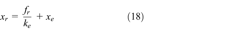
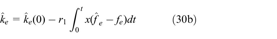
where the parameter f_r is set according to the actual contact situation. Therefore, the key to achieving a tracking target with zero force steady-state error is to be able to estimate or measure the environmental position x_e and environmental stiffness k_e in real time. The environmental position and stiffness are estimated online in real time, eliminating the environmental parameter errors mentioned above.

This will obtain a new reference trajectory for real-time tracking of the desired contact force.

As shown in Figure 3, using the indirect adaptive control method.²³ The desired position x_r is defined as:

x_{r} = \frac{f_{r}}{{\hat{k}}_{e}} + {\hat{x}}_{e}

(19)

where ${\hat{x}}_{e}$ and ${\hat{k}}_{e}$ are the real-time estimated values of x_e and k_e respectively.

Figure 3.

Diagram of adaptive impedance control model.

From the environmental contact model equation (12), we know

f_{e} = k_{e} (x - x_{e}) = k_{e} x - k_{h}

(20)

where $k_{h} = k_{e} x_{e}$ . According to ${\hat{x}}_{e}$ and ${\hat{k}}_{e}$ , the real-time estimated value of contact force ${\overset{⌢}{f}}_{e}$ is

{\hat{f}}_{e} = {\hat{k}}_{e} (x - {\hat{x}}_{e}) = {\hat{k}}_{e} x - {\hat{k}}_{h}

(21)

where ${\hat{k}}_{h}$ is the estimated value of k_h. Given $ϕ_{e} = {\hat{k}}_{e} - k_{e}$ , $ϕ_{h} = {\hat{k}}_{h} - k_{h}$ , and $ϕ = {[\begin{matrix} ϕ_{e} & ϕ_{h} \end{matrix}]}^{T}$ . From equations (20) and (21), we can see

ϕ = {[\begin{matrix} ϕ_{e} & ϕ_{h} \end{matrix}]}^{T}

(22)

when ${\hat{f}}_{e} = f_{e}$ , we can see from equations (19) and (21)

f_{e} = {\hat{k}}_{e} x - {\hat{k}}_{e} {\hat{x}}_{e} = {\hat{k}}_{e} (x - x_{r}) + f_{r}

(23)

Then

x - x_{r} = \frac{e}{{\hat{k}}_{e}}

(24)

Substituting equation (21) into the impedance model equation (8), we know

m \overset{\cdot\cdot}{e} + (b + k_{d} \hat{k_{e}}) \overset{\cdot}{e} + (k + k_{p} \hat{k_{e}}) e = 0

(25)

In the steady state, from equation (25), it can be seen that the condition of $(k + k_{p} {\hat{k}}_{e}) e = 0$ is e→0 or $(k + k_{p} {\hat{k}}_{e}) \to 0$ , According to the environmental stiffness $k_{e} > 0$ and ${\hat{k}}_{e} > 0$ , $(k + k_{p} {\hat{k}}_{e}) > 0$ is obtained. Since the force tracking error is $e = f_{e} - f_{r} = 0$ , where ${\hat{f}}_{e} \to f_{e}$ , $f_{e} \to f_{r}$ , the position tracking with zero force steady-state error is realized.

Using Lyapunov stability theory, design update algorithm of ${\hat{x}}_{e}$ and ${\hat{k}}_{e}$ to realize ${\hat{f}}_{e} \to f_{e}$ . Define the Lyapunov function as

V = ϕ^{T} Γ ϕ

(26)

where Γ is the second-order diagonal positive constant value matrix, $Γ = [\begin{matrix} 1 / r_{1} & 0 \\ 0 & \frac{1}{r_{2}} \end{matrix}]$ , r₁ and r₂ are positive scalar constant values.

According to the Lyapunov stability principle, to satisfy $\overset{\cdot}{V}$ is a negative definite. Define $\overset{\cdot}{ϕ}$ as

\overset{\cdot}{ϕ} = - Γ^{- 1} [\begin{matrix} x \\ - 1 \end{matrix}] (\hat{f_{e}} - f_{e})

(27)

then the derivative of the Lyapunov function along the direction $\overset{\cdot}{ϕ}$ is

\overset{\cdot}{V} = 2 ϕ^{T} Γ \overset{\cdot}{ϕ} = - 2 ϕ^{T} [\begin{matrix} x \\ - 1 \end{matrix}] (\hat{f_{e}} - f_{e}) = - 2 (\hat{f_{e}} - f_{e})

(28)

when the estimation error ϕ changes in the direction given by equation (27), the system converges near the equilibrium state. When $t \to \infty$ , ${\hat{f}}_{e} \to f_{e}$ , thus $f_{e} \to f_{r}$ .

Combining the definition of ϕ and formula (27), we can get

{\begin{matrix} \dot{\hat{k_{e}}} = - r_{1} x (\hat{f_{e}} - f_{e}) \\ \dot{\hat{x_{e}}} = \frac{\hat{f_{e}} - f_{e}}{\hat{k_{e}}} (r_{1} x \hat{x_{e}} + r_{2}) \end{matrix}

(29)

In summary, the adaptive controller for the desired position x_r is designed as follows

x_{r} = \frac{f_{r}}{{\hat{k}}_{e}} + {\hat{x}}_{e}

(30a)

{\hat{k}}_{e} = {\hat{k}}_{e} (0) - r_{1} \int_{0}^{t} x ({\hat{f}}_{e} - f_{e}) dt

(30b)

{\hat{x}}_{e} = {\hat{x}}_{e} (0) + \int_{0}^{t} \frac{{\hat{f}}_{e} - f_{e}}{{\hat{k}}_{e}} (r_{1} x {\hat{x}}_{e} + r_{2}) dt

(30c)

{\hat{f}}_{e} = {\hat{k}}_{e} (x - {\hat{x}}_{e})

(30d)

Control strategy

The industrial robot is combined with the end effector motion control, based on the adjustment of the contact force of the end effector and the control position of the industrial robot. Aiming at the grinding and polishing robot system scheme, a compliant motion control strategy is proposed. The control strategy is divided into two parts. The first part considers the process of robot moving to the workpiece in free space, the purpose is to reduce the impact force generated when the grinding and polishing robot hits the workpiece. The second part considers the end position, posture and force control adjustment when the robot is in contact with the workpiece and performs a compliant motion.

Impact control

The impact control is aimed at the working scene of the grinding and polishing robot and the workpiece from free space to stable contact. In Figure 4, when the grinding and polishing robot moves in the free space, the end effector contacts the workpiece with the required force through the impact control scheme. The position of the end effector is adjusted according to the contact force acting on it. When the position changes, the controller provides driving instructions for the voice coil motor module. Therefore, it is necessary to consider the linear motion range of the motor during the movement of the voice coil motor module. Define the middle position of the motor stroke as the motion reference position. It is also assumed that the distance between the workpiece and the grinding and polishing robot is unknown.

Figure 4.

Block diagram of impact control.

In Figure 4, the robot macro motion control algorithm is used to control the position of the grinding and polishing robot, and the robot micro motion control algorithm is used to switch to realize the position control and force control of the end effector. An appropriate amount of speed feedback adjustment is performed at the joints of the industrial robot. By reducing the speed of the robot’s macro motion, the energy and therefore the impact force are reduced. The grinding and polishing robot detects the contact force in real time through a force sensor to determine the contact state:

When the robot is not in contact with the workpiece, the end effector selects a larger k_pmi. It carries out position control with big rigidity to keep the motor position at the middle position of the motor stroke, which is the reference position P_r. When the grinding and polishing robot moves along the contour of the workpiece, the end effector is controlled in P_r to make the robot in the best working area.

When $f_{e} - f_{r} > η_{1} f_{r}$ is in contact with the workpiece, $η_{1}$ uses aluminum-aluminum friction coefficient of 0.2.²⁴ The end effector reduces k_pmi and position control stiffness. It performs a larger position movement while applying a smaller force. By reducing the speed of the robot’s macro motion, energy and impact are reduced.

When it is $f_{e} - f_{r} > η_{2} f_{r}$ , the industrial robot will maintain its position, and the robot micro-motion control algorithm will switch to the force control of the end effector. The robot macro motion almost stops.

The above is the process from free space to stable contact between the grinding and polishing robot and the workpiece. According to the specific material and application requirements of the workpiece, a is used as a contact sign to slow down the industrial robot, and b is a sign that the end effector is converted from position control to force control. When selecting other workpieces, you can fine-tune the above coefficients to obtain a good control effect.

Compliant control

The compliant motion control considers the process of stable contact between the grinding and polishing robot and the workpiece. It includes industrial robot pose control and end effector force control. The robot macro motion control algorithm makes the industrial robot move in accordance with the planned trajectory. The end effector maintains the required posture and force. The content of the control strategy is shown in Figure 5.

Figure 5.

Block diagram of compliance control.

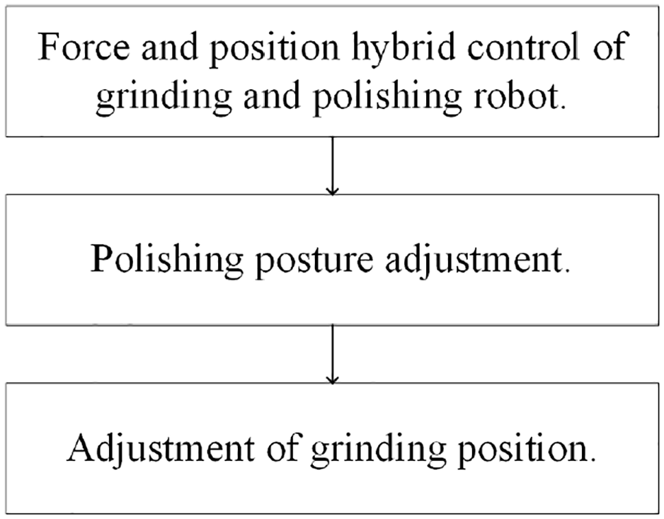
Force and position hybrid control of grinding and polishing robot

When the end effector is in contact with the workpiece, the grinding and polishing robot needs to be controlled to produce the desired motion and force. As shown in Figure 6, this paper draws on the idea of force/position hybrid control and introduces a selection matrix S to orthogonally decouple the task space into position free subspace and force constrained subspace. The axis of the force coordinate system and the position coordinate system are perpendicular, similar to the hybrid control of force/position. The industrial robot will move in the selected direction, the end effector adjusts the force applied to the workpiece through the impedance control method. The grinding and polishing robot uses force and position information for pose adjustment and end effector force control. The end effector keeps the reference position while realizing the tracking control of the complex curved surface.

Figure 6.

Control block diagram of force and position hybrid control.

In the control scheme, even if the workpiece has a large size error, the grinding and polishing robot still moves along the unknown workpiece contour without losing contact. When the changing speed of the workpiece geometry is within the bandwidth of the robot system, the ability to track the pose of the grinding and polishing robot can be achieved. Most of the time in the tracking control should be in the end effector force control to meet the requirements of rapid response.

Polishing posture adjustment

For tracking inclined surface of workpiece contour, this article adopts the idea of contact torque adjustment. It adjusts the end posture of the robot when the robot is in initial stable contact with the inclined surface. When moving along the inclined surface, only consider adjusting the attitude of the robot end relative to the inclined surface during the initial contact, and there is no need to adjust the attitude at other times.

The end force of the grinding and polishing robot is shown in Figure 7. b is the base coordinate system. v_n is the speed of the end of the robot, F_n is the normal pressure of the inclined surface. Φ₁ is the craft corner, Φ₂ is the angle of the inclined plane. Φ is the movement angle of the robot in base coordinate system, which is equal to the sum of Φ₁ and Φ₂. In the current posture, the torque generated by F_n at the end of the robot is M_n(k). Assuming that F_n can generate torque M_d at the end of the robot in the desired posture, then

e_{m} (k) = M_{d} - M_{n} (k)

(31)

Figure 7.

Contact schematic diagram of inclined surface.

The current robot end posture adjustment rotation matrix is ^TR(k+1) in the robot tool coordinate system, and the force sensor coordinate system coincides with the tool coordinate system T:

\begin{matrix} {}^{T}R (k + 1) = I + \frac{\sin θ}{‖ u ‖} S (u) + \frac{1 - \cos θ}{{‖ u ‖}^{2}} S^{2} (u) \\ k = 0, 1, 2, . . . \end{matrix}

(32)

where I is the unit matrix; u and θ are the equivalent rotation axis vector and rotation angle respectively; S(u) is the skew symmetric matrix function of the vector u.²⁵

Calculate θ(k+1) and u(k+1) according to the following expressions:

θ (k + 1) = k_{θ} | e_{m} (k) |

(33)

u (k + 1) = u (k) + k_{m} \frac{e_{m} (k)}{| e_{m} (k) |}

(34)

where k_m and k_θ are constant coefficients.

It is easy to know that ^TR(k+1) can be expressed as:

{}^{b}R (k + 1) = {}_{T}^{b}R (k)^{T} R (k + 1)

(35)

where ${}_{T}^{b}R$ is the rotation transformation matrix of the robot tool coordinate system relative to the base coordinate system, then

{}^{b}T (k + 1) = {}^{b}R (k + 1)^{b} T (k)

(36)

where ^bT(k) is the current pose matrix of the robot end. Substituting ^bT(k+1)) into the inverse kinematics solution can obtain the robot joint angular displacement value of the desired posture. The robot macro motion control algorithm realizes the desired posture of the robot end adjustment.

Adjustment of grinding position

After the end of the grinding and polishing robot adjusts its posture and makes stable contact with the inclined surface, the end effector sends its displacement information to the industrial robot during the force control process. When the displacement of the end effector is far away from the set reference position, the existing displacement error is converted into a displacement compensated by the industrial robot. This puts the end effector at the reference point position.

The displacement error of the end effector is:

e_{pos} = P_{r} - P_{mi}

(37)

e_{mi} = [\begin{matrix} 0 \\ 0 \\ e_{pos} \end{matrix}]

(38)

where P is a position vector of 1 × 1 order; P_r and P_mi are the reference point position and actual displacement of the end effector. Considering that the end effector itself has 1 degree of freedom, the position error is represented by the scalar e_pos at this time. The displacement error of the end effector in space should be represented by a position error vector of 3 × 1. Assuming that the end effector moves toward the z-axis relative to the end coordinate system of the grinding and polishing robot at this time, e_pos is transformed into e_mi. The displacement error of the end effector is compensated by the industrial robot, and we can get:

{}^{b}T (k + 1) = {}_{T}^{b}T (k) {e_{mi}}^{b} T (k)

(39)

where ${}_{T}^{b}T$ is the transformation matrix of the robot tool coordinate system relative to the base coordinate system, and ^bT(k) is the current pose matrix of the robot end. Substituting ^bT(k+1) into the inverse kinematics solution can obtain the robot joint angular displacement value, which is realized position error compensation of the end effector.

Simulation and analysis

According to the polishing process, the control strategy of the polishing robot is proposed to enhance the smooth motion performance of the polishing system. The MATLAB simulation platform is used to simulate the motion control of the grinding and polishing robot system. In the grinding process, it is usually considered to process in the normal direction of the workpiece, where the simulation processing direction is the normal direction of the workpiece. Furthermore, in the hardware part of this paper, a single degree of freedom end effector is designed. Considering the motion of the end effector, only the single direction motion is discussed. In order to verify the feasibility of the macro and micro force position hybrid control strategy for grinding and polishing robot, this paper avoid the complexity of three-dimensional posture and position simulation. The simulation assumes that the posture of the macro robot remains unchanged, and only considers the constraints such as the change of the normal position of the macro robot.

Robot micro motion control simulation

Position tracking

A single-direction position correction is performed on the micro-motion of the robot to verify whether the adaptive impedance control model can adapt to changes in the environment.²⁶ Assuming that the end position x of the robot is the same as the desired position x_r, the error caused by the robot macro motion position control system is ignored. The environmental stiffness in the simulation can be selected according to the actual processing conditions. This article selects the processed aluminum parts. Table 1 shows the specific simulation parameters.

Table 1.

Simulation parameters of adaptive impedance.

Simulation parameters	Value
m	3 kg
b	500 N/(m/s)
k	5000 N/m
k_e	7000 N/m
${\hat{k}}_{e} (0)$	5000 N/m
${\hat{x}}_{e} (0)$	0 m
r ₁	5
r ₂	10
f _r	5 N
sampling time	1 ms

Figure 8 shows the simulation of the designed adaptive control system performance in MATLAB/Simulink. Table 2 shows the simulation parameters of displacement tracking under different conditions. Because the simulation is aimed at the force control algorithm and the corresponding control strategy, the movement of the end effector is mainly simulated. In order to show the dynamic model of the end effector, the voice coil motor subsystem is added in Figure 8. According to the characteristics of voice coil motor, the voice coil motor subsystem is modeled as DC motor, and the parameters are assigned according to the actual situation. In the Figure 8, R is the resistor, l is the inductor, Km is the torque constant, Kemf is the back EMF voltage constant, Kf is the viscous friction constant, and J is the inertial load. Values have been set experimentally to the following values: R = 2; L = 0.5; Km = 0.1; Kemf = 0.1; Kf = 0.2; J = 0.02. PID (s) is set according to section 2.3.1.

Figure 8.

Simulink position tracking simulation model.

Table 2.

Position tracking working condition parameter.

Number	x _e(0) (m)	k _e(0) (N/m)	x _e(1.5 s) (m)	k _e(1.5 s) (N/m)
a	0.01	7000	0.01	7000
b	0.01	7000	0.005*sin(πt)	7000
c	0.01	7000	0.011	7000
d	0.01	7000	0.01	3000

Impedance control and adaptive impedance control are used for position tracking under different working conditions. Figure 5 shows the simulation of Simulink position tracking under different working conditions. Table 3 shows the simulation result data.

Table 3.

Simulation results of position tracking under different working conditions.

Method	Impedance control		Adaptive impedance control
Number	Average (m)	Standard deviation (m²)	Average (m)	Standard deviation (m²)
a	0.00379	0.000556	0.000907	0.000104
b	0.00127	0.000699	0.000715	0.000129
c	0.00401	0.000566	0.000903	0.00104
d	0.00469	0.000997	0.00138	0.00106

In Figure 9(a), when the environment position and stiffness remain unchanged, impedance control can achieve stable position tracking. The control system cannot accurately track the environmental position due to the error between the expected position and the environmental position. It can be seen from the average value of the two errors in Table 3 that the adaptive impedance control can achieve a smaller error tracking of the environmental position when the environmental position and stiffness are unchanged.

Figure 9.

Simulink simulation of position tracking under different working conditions: (a) constant position and rigidity, (b) continuous change in position, (c) sudden change in position, and (d) sudden change in stiffness.

In Figure 9(b), the environment position changes with a sine law. Impedance control has lost the ability to track the environment position stably, while adaptive impedance control can still better track the environment position. In Table 3, although the average value of impedance control error is only 0.00127 m, the corresponding standard deviation is relatively large, and the tracking process is unstable.

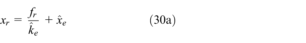
In Figure 9(c), the location of the environment changes suddenly. Compared with the standard deviations of the two methods in Table 3, the impedance control transient response is faster. In their average error comparison, the adaptive impedance control environment position tracking error is small. From equation (30a), we know that we need to pay attention to the value of the desired force f_r. If f_r is too small, it is expected that the update of the position will be slow, so that it cannot respond quickly to changes in the environmental position. This shortcoming can be solved by appropriately increasing f_r, but if f_r is too large, the system will produce tracking errors of the environmental position. The value of f_r needs to be determined according to actual requirements.²⁷

Figure 9(d) reflects the position tracking performance when the environmental stiffness changes suddenly. When the environmental stiffness changes suddenly, it can be seen from Table 3 that the response speed of adaptive impedance control is faster than impedance control, and the adjustment time is shorter. Figure 9(d) shows that the sudden change of environmental stiffness has an impact on the position tracking result of adaptive impedance control.

Position tracking

Table 2 is a parameter table of different working conditions. The adaptive impedance control simulates the contact force of the robot’s micro-motion, and the expected force $f_{r} = 5$ . Figure 10 shows the Simulink simulation model of force estimation under different working conditions, and the simulation results are shown in Figure 11. The allowable error range of the force estimation curve is 1% of the expected force. Table 4 shows the statistical results of the simulation data.

Figure 10.

Simulink force tracking simulation model.

Figure 11.

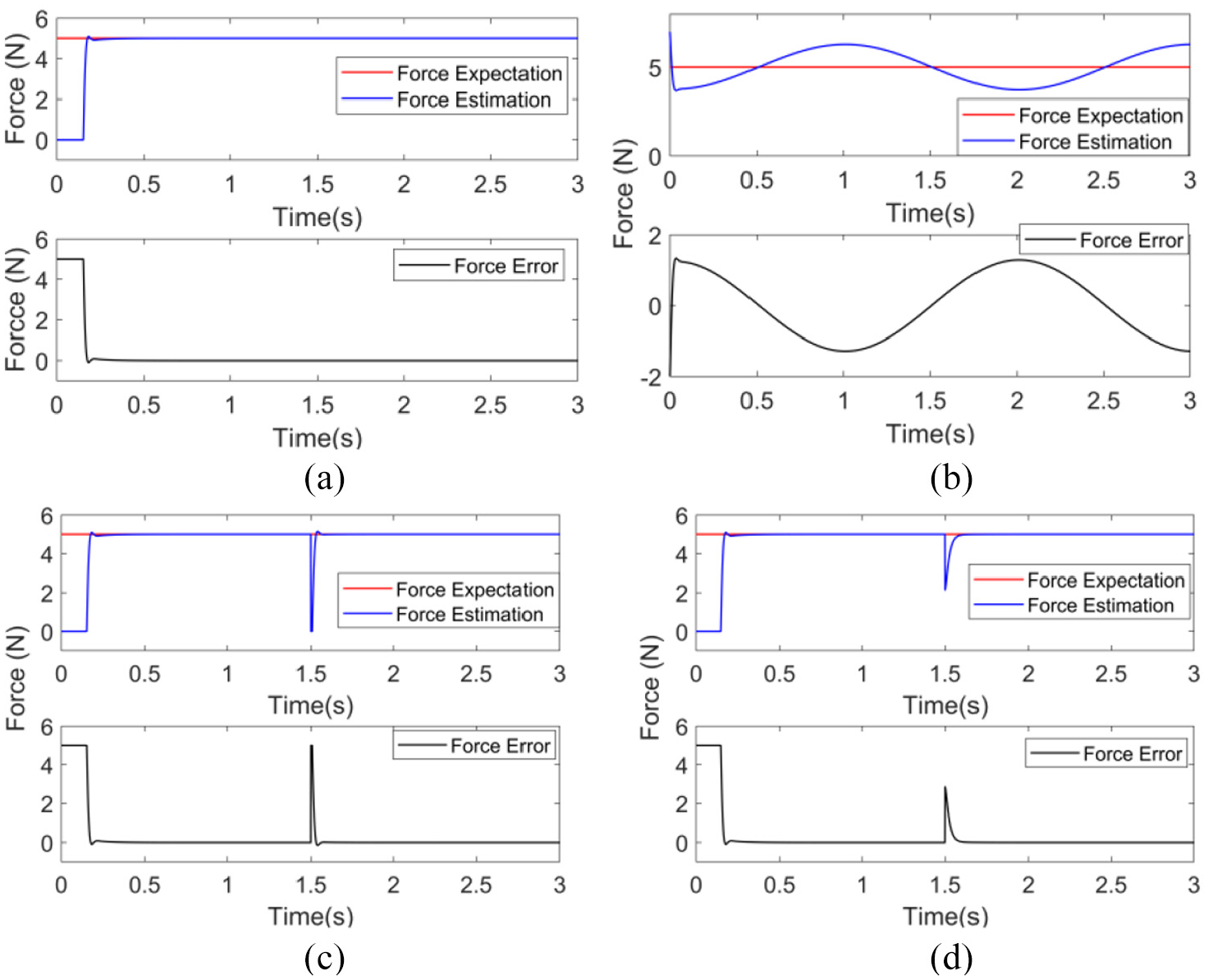
Simulink simulation results of force estimation under different working conditions: (a) constant position and rigidity, (b) continuous change in position, (c) sudden change in position, and (d) sudden change in stiffness

Table 4.

Statistics of force estimation simulation results under different working conditions.

Method	Impedance control		Adaptive impedance control
Number	Average (m)	Standard deviation (m²)	Average (m)	Standard deviation (m²)
a	4.734	1.103	5	0.269
b	5.004	0.905	1.99	–
c	4.707	1.145	5	0.192
d	4.708	1.115	2.851	0.221

In Figure 11(a), when the environment position and stiffness remain unchanged, the adaptive impedance control contact force estimate f_e converges to the desired force f_r. In Figure 11(b), when the environmental position changes in a sinusoidal law, the adaptive impedance control produces a larger force estimation error. It can be seen from equation (30a) that the force estimation error will increase with position error under the condition of constant environmental stiffness. The expected force can be estimated by reducing the position tracking error.

Figure 11(c) and (d) show that large force estimation errors will be caused, when the environment position or the environment stiffness changes suddenly. The environmental position increased from 0.01 to 0.011 m, resulting in a 10% change, corresponding to a force estimation error of 5 N. The environmental stiffness is reduced from 7000 to 3000 N/m, resulting in a 57% change, corresponding to a force estimation error of 2.851 N. The comparison shows that for a given f_r, a sudden change in the environmental position produces a greater contact force error.

Figure 11 shows that under different working conditions, f_e will convergences to f_r. This proves that the stability analysis conclusion described above is correct.

Impact control

The purpose of this experiment is to control the contact process between the grinding and polishing robot and the workpiece. In this process, through limited workpiece position information, the contact force will be controlled to the desired value and a small impact force will be generated.

It is assumed that the position control of the robot is error-free. In Figure 7, v_n is the end speed of the robot along the inclined plane, which can be equivalently replaced by the environment position change speed v_e in the control simulation. The impact force during the contact between the grinding and polishing robot and the workpiece is simulated and analyzed in Matlab/Simulink. Table 5 shows the simulation parameter table of the impact force during the robot contacting the workpiece.

Table 5.

Simulation parameter of impact force during robot contact with workpiece.

Simulation parameters	Value
x_e(0)	0.01 m
v_e	0.001 m/s
k_e(0)	0 N/m
k_e(1.5 s)	7000 N/m
f_r	5 N
Sampling time	1 ms

Figure 12 shows the simulation of the grinding and polishing robot contacting the workpiece. The maximum contact force generated by the collision was taken when environmental stiffness changes into 7000 N/m at 1.5 s, and it is 220 N. The impact force control is used to handle the larger impact force in Figure 12.

Figure 12.

Simulink simulation of impact force during robot contact with workpiece.

Table 5 shows the simulation conditions. The impact force control considers adjusting the size of the contact force, and uses the environmental stiffness change speed k_e(1.5 s) as the variable design experiment. Setting k_e(1.5 s) to the environmental stiffness 1/20, 1/10, 1/5, and 1/2 as the environmental stiffness change rate, and the values are 350, 700, 1400, and 3500 N/m/s.

In the description of impact control, $η_{1} = 0.2$ is a contact mark, and $η_{2} = 0.6$ is a mark that the end effector position control is converted to force control. v_e is changed according to the control strategy in section 2.1. When the contact force increases to (1.2 f_r) 6 N, v_e begins to decrease. When the contact force increases to (1.6 f_r) 8 N, the desired position of environment stops and v_e is zero. The Simulink simulation results of the impact force control experiment for different environmental stiffness change speeds are shown in Figure 13, and the simulation results are shown in Table 6.

Figure 13.

Simulink simulation of stiffness change speed in different environments: (a) k_e(1.5 s) = 350 N/m/s, (b) k_e(1.5 s) = 700 N/m/s, (c) k_e(1.5 s) = 1400 N/m/s, and (d) k_e(1.5 s) = 3500 N/m/s

Table 6.

Simulation results of stiffness change speed in different environments.

Number	k _e(1.5 s) (N/m/s)	Position error (m)	Maximum force error (N)	Force sdjustment time (s)
a	350	0.0873	7.57	3.079
b	700	0.0849	10.86	2.184
c	1400	0.0837	15.65	1.905
d	3500	0.0832	25.41	0.985

Figure 13(a) corresponds to 350 N/m/s for k_e(1.5 s). When the force estimation is η₁ or 6 N, the desired position curve becomes slow. When the force estimation is η₂ or 8 N, the desired position stagnates or even decreases. When the force estimation meets the desired value, the slope of the desired position curve recovers and moves according to v_e. The force estimation and position estimation finally converged to the desired value. The initial part of the force estimation curve is 0 N as the non-contact area, which satisfies the definition of contact force in equation (12). When k_e(1.5 s) increases to 700 N/m/s, it can be seen from Table 6 and Figure 13(a) and (b) that the force estimation curve becomes narrower and higher. This shortens the corresponding adjustment time and increases the force error.

Figure 13(c) and (d) show that with k_e(1.5 s) increases, the force error increases, but the corresponding environmental error is stable. It can be seen from the above that the same workpiece and the same working condition have little effect on the position error when the environmental stiffness changes.

In Table 6, k_e(1.5 s) increases and the adjustment time becomes shorter. The position error is reduced, the range is 0.041 m, and the corresponding force error gradually increases, the range is 17.84 N. In the impact control, considering the force adjustment time, the environmental stiffness change speed is selected to be 1400 N/m/s. When the environmental stiffness changes suddenly, the contact force is within the safe force range of the sensor, and the contact force can quickly remain stable. In addition, the desired position of the robot can quickly track the change of the environment position, and the error adjustment ability is strong.

Compliant control

When the contact force is stable, the robot moves on the surface of the workpiece according to the compliant control. According to the force/position hybrid motion control algorithm, the end of the industrial robot moves parallel to the surface of the workpiece, and the end effector performs force control perpendicular to the surface of the workpiece. The end effector will eventually reach the limit of its working space and lose contact force. For compliance control in section 2.2, when the end effector force control process is displaced, the industrial robot obtains the displacement value of the force control direction. The industrial robot moves perpendicular to the surface of the workpiece to keep the end effector at the reference position. During this process, the end effector maintains contact and does not lose contact force.

It is assumed that the position control of the robot is error-free. Figure 14 shows the compliant control simulation in MATLAB/Simulink, and Table 7 shows the corresponding simulation parameters.

Figure 14.

Simulink compliance control simulation.

Table 7.

Compliance control simulation parameter.

Simulation parameters	Value
x_e(0)	0.01 m
v_e	–
k_e(0)	0 N/m
k_e(1.5 s)	1400 N/m
f_r	5 N
Sampling time	1 ms

Considering the tracking of the inclined surface of the workpiece, the angle of the inclined surface is expressed by the environmental position change speed v_e. The simulation is designed with v_e as a variable, taking 0.001, 0.005, 0.01, and 0.05 m/s to simulate processing conditions. When the environment position changes in different speeds, adaptive impedance control is used to obtain the position displacement during the control process. Figure 15 shows the Simulink simulation experiment of speed compliance with different environment position changes, and Table 8 shows the simulation results.

Figure 15.

Simulink simulation of different environment position change speed: (a) v_e = 0.001 m/s, (b) v_e = 0.005 m/s, (c) v_e = 0.01 m/s, and (d) v_e = 0.05 m/s

Table 8.

Simulation results of changing speed of different environmental position.

Number	v _e (m/s)	Maximum position error (m)	Force steady state error (N)	Force adjustment time (s)
a	0.001	0.0089	0.064	1.541
b	0.005	0.0089	0.393	0.947
c	0.01	0.0089	0.804	0.807
d	0.05	0.00909	3.966	1.545

When v_e is 0.001 m/s and k_e(1.5 s) is 1400 N/m/s for compliant motion control, the force estimation and position estimation of Figure 15(a) converge on the expected value. As shown in Table 8 and Figure 15(b), when v_e increases, the position estimation curve is similar to that of Figure 15(a), and the corresponding position error is the same. However, the steady-state error of the force estimation curve becomes larger and the adjustment time becomes shorter.

As shown in Figure 15(c) and (d), during the process of increasing the speed of environmental position change, the corresponding environmental position error is stable, but the steady-state error of the force gradually increases. It can be seen from (30d) and (30b) that when the environmental position error is stable, the change of the environmental position will cause the estimation force to increase. This is in line with the situation that the force estimation in the table increases with the increase of the environment position speed.

In Table 8, when v_e increases, the force adjustment time becomes shorter. The position error does not change much, the range is 0.00019 m, and the corresponding force steady-state error range is 3.902 N. Figure 15 shows that the robot and the workpiece are in stable contact. As v_e increases, the force stabilizes in a short time, but the steady-state error of the estimated force increases. Considering that the reference force is 5 N, the maximum position error and the steady-state error of the force are in a reasonable range when the ring v_e is less than 0.01. During the machining process, the environment position change speed less than 0.01 m/s can be selected to set the grinding and polishing speed parameters.

Experiment

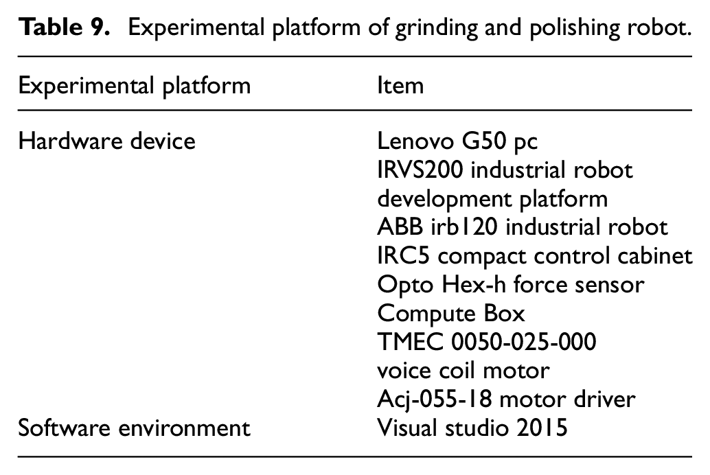
In order to verify the hybrid control method of macro and micro force and position of grinding and polishing robot, the control experiment is carried out on the system platform. As the macro micro motion control method of the grinding robot is established in the control strategy, the joint control of the industrial robot and the end effector is carried out. In this section, the effectiveness of the method will be verified through the contact force and the macro micro motion trajectory. The composition of the experimental platform is shown in Table 9.

Table 9.

Experimental platform of grinding and polishing robot.

Experimental platform	Item
Hardware device	Lenovo G50 pc
	IRVS200 industrial robot development platform
	ABB irb120 industrial robot
	IRC5 compact control cabinet
	Opto Hex-h force sensor
	Compute Box
	TMEC 0050-025-000 voice coil motor
	Acj-055-18 motor driver
Software environment	Visual studio 2015

After the robot is powered on and enabled, the robot switches to the manual mode to control the robot to return to the origin. At this time, the grinding tool and the workpiece are in a non-contact state. When the motion mode is switched to the automatic mode, the robot starts to read and run the trajectory taught in advance, as shown in Figure 16.

Figure 16.

Robot grinding and polishing experiment path.

The initial position of robot is the teaching point 0. The robot moves from the teaching point 0 to the teaching point 1, and then to the teaching point 2, and the force control in z direction is turned on. The robot position in z direction remains unchanged. At this time, the grinding head and the workpiece have not contacted, and the end effector will make the grinding head fit with the workpiece and maintain the desired contact pressure under the force control. At the same time, the robot moves back and forth between teaching point 3 and teaching point 2 along the tangential direction (x direction) of the workpiece under the position control. The actual contact force between grinding head and workpiece in the whole grinding process is collected and analyzed. The sampling period of force sensor is 5 ms.

On the experimental platform described in Table 9, the performance of the macro micro force position hybrid control method in the grinding process is verified. The effectiveness of the method is verified by the motion trajectory and contact force. In this section, the contact force between the grinding head and the workpiece is set as 10 N, and the tangential movement speed in x-axis is 10 mm/s. The actual contact force between the grinding head and the workpiece during the grinding process is collected. There are protrusions on the surface of the workpiece, and only the coordinates of the starting point of the trajectory are given in the RAPID program.

During the experiment, the surface condition of the workpiece is unknown. According to the hybrid control method of macro micro force and position, the real-time position of the industrial robot and the end effector can be superimposed as the surface position of the workpiece. In the experimental results, the z-axis macro motion and micro motion position of the end effector of the robot are shown in Figure 18. The abscissa represents the number of sampling periods, and the ordinate represents the position of each part of the robot.

The machining path can be obtained by superposing the two position curves in Figure 17, and the millimeter level shape of the actual workpiece surface can be estimated by the machining path, as shown in Figure 18.

Figure 17.

Position of each part of robot in grinding and polishing process.

Figure 18.

Estimation of millimeter surface topography of workpiece.

After obtaining the estimation of workpiece surface topography, it is necessary to verify the workpiece surface condition. When the robot moves to the teaching point 2, the self-locking of voice coil motor is turned off, so that the end effector and the workpiece surface are always in a state of contact. The experimental results are shown in Figure 19. The ordinate represents the contact force between the grinding head and the workpiece.

Figure 19.

Contact force change without force control process.

In Figure 18, we can see that there are three bumps larger than 325 mm in the surface profile estimation curve, and the peaks appear at the 7500th, 13,440th and 18,580th sampling periods respectively. It shows that in the process of robot grinding and polishing, large contact forces are detected at these three positions, and the corresponding position adjustment are carried out.

It can be seen from Figure 19 that the contact force is not kept at 0 N during the movement without force control, which is due to certain deformation on the surface of the workpiece. As shown in Figure 19, the peak values of the contact force at the two bulges are 1.815 and 1.465 N. There are two peaks in the contact force curve, and the convex peaks appear in the 6960th and 17,580th sampling periods respectively. Through the comparison between Figures 18 and 19, the corresponding period of curve convex peak is basically the same, so the estimated workpiece surface position is basically consistent with the actual position. The experimental results show that the force control algorithm can effectively estimate the millimeter level surface topography of the workpiece.

Turn on the force control, carry out the experiment under the same conditions of other experiments, and collect the force in z direction of the sensor. The force control algorithm adopts adaptive impedance control, and the parameters are obtained by measurement during the experiment. The value of k is 2877.5 N/m, b is 220.36 N/ (m/s), and m is 1.4 kg.

The contact force curve of force control experiment is shown in Figure 20, the position curve of each part is shown in Figure 21, and the displacement curve of grinding and polishing robot is shown in Figure 22. According to the change of contact force, the curve is divided into five segments. In segment 1, before the end effector contacts the workpiece, the macro motion of the robot generates the contact force. Segment 2 is the process of the end effector contacting the workpiece, in which the micro motion of the end effector produces the contact force. Segment 3 is the process of the robot moving when the workpiece bulges, and the macro micro cooperative movement. Segment 4 is the stable operation process of the grinding and polishing robot. In Segment 5, the grinding robot ends its motion, and the end effector moves for force control.

Figure 20.

Change of contact force in force control process.

Figure 21.

Displacement of grinding and polishing robot in force control process.

Figure 22.

Displacement of grinding and polishing robot in force control process.

The force and displacement of the above five parts are shown in Table 10.

Table 10.

Force and displacement statistics of grinding and polishing process.

Number	Relative error of contact force (N)	Relative displacement of macro motion (mm)	Relative displacement of micro motion (mm)
1	3.48	0.001	0.042
2	3.43	0.001	0.039
3	3.93	0.001	0.096
4	2.92	0.003	0.398
5	3.69	0	0.115

It can be seen from Table 10 and Figures 20 to 22 that in segment 1, the robot first performs macro motion to generate contact force, and then the end effector performs high-frequency displacement adjustment. The amplitude of contact force curve is 3.48 N. In segment 2, the displacement adjustment of the end effector is less than that of the segment 1, and the amplitude of the contact force curve decreases to 3.42 N. In segment 3, when the grinding head is on the convex part of the workpiece surface, the adjusting displacement of the end effector increases, and the amplitude of the corresponding contact force increases to 3.93 N. Compared with the first two segments, the amplitude of contact force changes little, so the force control algorithm is effective. In segment 4, the robot realizes the stable grinding process. When the relative displacement of macro and micro motion increases, the contact force curve is stable, and the contact force is stable at 10 ± 3 N. In segment 5, the robot is in the end position of the trajectory, the macro motion stops first, and the micro motion is adjusted until the contact force is 0 N to end the grinding and polishing process.

The experimental results show that the hybrid algorithm can estimate the millimeter level surface topography of the actual workpiece by machining trajectory, and it is effective for force control of unknown surface contact process. As for the error of force tracking, it can be considered that the force control is realized by using the secondary development interface of the robot. The controller of the robot system is closed and cannot directly modify the reference position. It can only send the robot control system to move to the relevant point through the interface, which reduces the real-time performance of the force control command.

Conclusions

For the grinding and polishing robot system, an electrically driven end effector is designed to meet the needs of the system and to carry out a lightweight design. In addition, the digital axis modeling method is used to establish a model of the grinding and polishing robot system in contact with the environment. Through the discussion of the control model combined with the system dynamics and the impedance control method, the macro and micro motion control model of the grinding and polishing robot is established.

Aiming at the impact process of grinding and polishing, the active compliance method is adopted to establish impact control and compliance control strategies. The rough position information of the workpiece is used to realize the contact process of the workpiece through impact control, and the contact of the workpiece with unknown contour can be realized through the compliant motion control. Finally, the adaptive force control and position tracking control of grinding and polishing processing are realized.

The algorithm is verified by Simulink simulation and experiment. In MATLAB/Simulink, the control model, impact control and compliance control are simulated under different working conditions to verify the performance of force control and position tracking. The simulation results show that when the environmental stiffness change speed is 1/5 of the environmental stiffness and the environmental position change rate is less than 0.01, the position tracking error of the end effector does not exceed 0.009 m, and the force steady state error is less than 1 N. Through the grinding experiment of the workpiece, the effectiveness of the hybrid control strategy is verified. The motion curve is consistent with the surface morphology of the workpiece, and the contact force is stable at 10 ± 3 N. The experimental results show that the hybrid algorithm can estimate the millimeter level surface topography of the actual workpiece by machining trajectory, and it is effective for force control of unknown surface contact process.

Footnotes

Handling Editor: James Baldwin

Author contributions

Conceptualization, H.Z. and Z.L.; Data curation, Y.Z.; Formal analysis, H.Z. and S.M.; Funding acquisition, H.Z.; Investigation, G.W.; Methodology, S.M.; Project administration, Z.L.; Resources, Z.L.; Software, S.M.; Supervision, Z.L.; Validation, G.W.; Visualization, Y.Z.; Writing—original draft, H.Z. and S.M.; Writing—review & editing, S.M. All authors have read and agreed to the published version of the manuscript.

Declaration of conflicting interests

The author(s) declared no potential conflicts of interest with respect to the research, authorship, and/or publication of this article.

Funding

The author(s) disclosed receipt of the following financial support for the research, authorship, and/or publication of this article: This work was supported by National Key R&D Program of China (2018YFB1308900), Natural Science Foundation of Tianjin (18JCYBJC20100).

ORCID iD

Zhenzhong Liu

References

Mohammad

AEK

Wang

. Electrochemical mechanical polishing technology: recent developments and future research and industrial needs. Int J Adv Manuf Technol 2016; 86: 1–16.

Zhang

Liu

, et al. A survey of robotic polishing. In: 2018 IEEE international conference on robotics and biomimetics (ROBIO), Kuala Lumpur, Malaysia, 12–15 December 2018. IEEE.

Fang

Zhang

, et al. Modeling and force control of robotic polishing system for the wheel hubs*. In: Robotics and biomimetics (ROBIO) 2019 IEEE international conference, Dali, Yunnan, China, 6–8 December 2019. IEEE.

Roswell

Liu

Modelling and analysis of contact stress for automated polishing. Int J Mach Tools Manuf 2006; 46: 424–435.

Raibert

Craig

Hybrid position/force control of manipulators. J Dyn Syst Meas Control 1981; 103: 126–133.

Roveda

Pedrocchi

Beschi

High-accuracy robotized industrial assembly task control schema with force overshoots avoidance. Control Eng Pract 2018; 71: 142–153.

Duan

Gan

Chen

Adaptive variable impedance control for dynamic contact force tracking in uncertain environment. Rob Auton Syst 2018; 102: 54–65.

Dong

Ren

UDE-based variable impedance control of uncertain robot systems. IEEE Trans Syst Man Cybern 2019; 49: 2487–2498.

Martinmartin

Lee

Gardner

. Variable impedance control in end-effector space: an action space for reinforcement learning in contact-rich tasks. In: 2019 IEEE/RSJ international conference on intelligent robots and systems (IROS), Macau, China, 3–8 November 2019. IEEE.

10.

Hogan

Impedance control: an approach to manipulation: part I—theory. J Dyn Syst Meas Control 1985; 107: 1–7.

11.

Tan

Jiang

Zhang

. Instantaneous-model impedance control based on hybrid position controller. In: Technology networking electronic and automation control conference (ITNEC) 2017 IEEE 2nd information, ChengDu, China, 15–17 December 2017. IEEE.

12.

Zhao

Paine

Jorgensen

, et al. Impedance control and performance measure of series elastic actuators. IEEE Trans Ind Electron 2018; 65: 2817–2827.

13.

Ozgoli

Taghirad

HD.

A survey on the control of flexible joint robots. Asian J Control 2008; 8: 332–344.

14.

Tsumugiwa

Yura

Kamiyoshi

, et al. Development of mechanical-impedance-varying mechanism in admittance control. J Rob Mechatron 2018; 30: 863.

15.

Hong

Ang

, et al. Design and control of an end-effector module for industrial finishing applications. In: 2016 IEEE international conference on advanced intelligent mechatronics (AIM), Banff, AB, Canada, 12–15 July 2016. IEEE.

16.

Mohammad

AEK

Hong

Wang

Design of a force-controlled end-effector with low-inertia effect for robotic polishing using macro-mini robot approach. Rob Comput Integr Manuf 2018; 49: 54–65.

17.

Tol

Clerc

Wiens

. Micro/macro approach for dexterity enhancement of PKM. In: Proceedings of the WORKSHOP on fundamental issues and future research directions for PKM, Quebec, Canada, 3–4 October 2002.

18.

Jamisola

Oetomo

Ang

MH.

Compliant motion using mobile manipulator: an operational space formulation approach to aircraft canopy polishing. Adv Robo 2005; 19: 613–634.

19.

Duan

Han

, et al. Multi-interactive control based on force/position/impedance of robotic arm in unknown environment. Robot 2017; 39: 449–457.

20.

Arifin

Ang

Lai

, et al. General framework of the force and compliant motion control for macro mini manipulator. In: 2013 IEEE/ASME international conference on advanced intelligent mechatronics, Wollongong, NSW, Australia, 9–12 July 2013. IEEE.

21.

Murray

. A mathematical introduction to robotic manipulation. Boca Raton, FL: CRC Press, 1994.

22.

Hong

Ang

, et al. A force control method with positive feedback for industrial finishing applications. In: 2018 IEEE/ASME international conference on advanced intelligent mechatronics (AIM), Auckland, 9–12 July 2018. Piscataway: IEEE.

23.

Seraji

Richard

Force tracking in impedance control. Int J Rob Res 1997; 16: 97–117.

24.

Chen

Selection and optimization of abrasive grain size during grinding. Metrol Test Technol 2018; 45: 8–10+ 14.

25.

Song

A Study of force and position tracking control for robot contact with an arbitrarily inclined plane. Int J Adv Rob Syst 2013; 10: 69–76

26.

Chen

Gao

Pan

Novel door-opening method for six-legged robots based on only force sensing. Chin J Mech Eng 2017; 5: 124–134.

27.

Xing

Ding

Gao

Adaptive tracking of axial position for valve-turning with a robot based on impedance control. Chin J Mech Eng 2019; 15: 124–134.

A hybrid control strategy for grinding and polishing robot based on adaptive impedance control

Abstract

Keywords

Introduction

System modeling

Structural design

Robot macro motion control

Robot micro motion control

PD control

Adaptive impedance control

Control strategy

Impact control

Compliant control

Force and position hybrid control of grinding and polishing robot

Polishing posture adjustment

Adjustment of grinding position

Simulation and analysis

Robot micro motion control simulation

Position tracking

Position tracking

Impact control

Compliant control

Experiment

Conclusions

Footnotes

Author contributions

Declaration of conflicting interests

Funding

ORCID iD

References