Well-balanced finite volume multi-resolution schemes for solving the Ripa models

Abstract

In this article, fifth order well-balanced finite volume multi-resolution weighted essentially non-oscillatory (FV MR-WENO) schemes are constructed for solving one-dimensional and two-dimensional Ripa models. The Ripa system generalizes the shallow water model by incorporating horizontal temperature gradients. The presence of temperature gradients and source terms in the Ripa models introduce difficulties in developing high order accurate numerical schemes which can preserve exactly the steady-state conditions. The proposed numerical methods are capable to exactly preserve the steady-state solutions and maintain non-oscillatory property near the shock transitions. Moreover, in the procedure of derivation of the FV MR-WENO schemes unequal central spatial stencils are used and linear weights can be chosen any positive numbers with only restriction that their total sum is one. Various numerical test problems are considered to check the validity and accuracy of the derived numerical schemes. Further, the results obtained from considered numerical schemes are compared with those of a high resolution central upwind scheme and available exact solutions of the Ripa model.

Introduction

The shallow water equations (SWEs) are of great importance due to wide range applications in incompressible flows, such as bore propagation, solute transport, currents in estuaries, and in surges or tsunamis phenomenon. The Ripa model comprises the SWEs and terms which account for horizontal temperature fluctuations. This shows that the study of Ripa models is of great importance to understand the various real-world phenomenon. Initially, the Ripa model was presented in Refs.^1–3 to analyze the ocean currents. The governing equations of this model were derived by integrating the velocity field, density, and horizontal gradients along the vertical direction in each layer of multi-layered models.^3,4 Recently, different numerical schemes are introduced to solve the Ripa models, see for instance.^4–9 Meanwhile, the exact solutions of Riemann problems for one-dimensional Ripa models with flat and non flat bottom topographies are computed in Rehman and Qamar. ¹⁰ The basic idea for constructing exact solutions in Rehman and Qamar ¹⁰ have been taken from Refs.^11–13 All the aforementioned numerical techniques for the Ripa models are at most second order accurate except the one presented in Han and Li. ⁶ Han and Li ⁶ the authors have used high order finite difference schemes based on WENO limiters ¹⁴ for solving the Ripa model. However, the finite difference schemes have some limitations. For examples, the finite volume numerical techniques enforce the conservation of flow variables at the discretized level and such types of techniques are easily formulated for the unstructured grid systems.

Due to the importance of nonlinear hyperbolic conservation laws, lot of high order numerical schemes have been designed to solve these laws. Among them, essentially non-oscillatory (ENO) and weighted essentially non-oscillatory schemes have been applied successfully to solve these conservation laws in one, two, and three dimensions. First of all, Harten and Osher ¹⁵ developed FV ENO numerical scheme that used an adaptive stencil based on smooth indicators. This scheme resolved the sharp discontinuities efficiently and ensured high order accuracy in the smooth areas. After that, Shu and Osher^16,17 introduced finite difference ENO schemes in 1988 and 1989. Subsequently, Liu et al. ¹⁸ introduced the third order FV WENO numerical scheme which is improved version of FV ENO scheme. In this FV WENO scheme, they improved the order of accuracy and used the convex combination of all the candidate stencils. Later, Jiang and Shu ¹⁹ developed high order finite difference WENO numerical schemes. Since then, these numerical schemes are being developed, modified, and extended for different fields of science and engineering, for detail see Refs.^20–30 Also well-balanced finite difference and finite volume WENO schemes^6,14,31–33 are developed for compressible and incompressible fluid flows.

In this article, fifth order well-balanced finite volume multi-resolution WENO schemes are constructed for solving the one-dimensional (1D) and two-dimensional (2D) Ripa models with and without source terms. We borrow the idea of MR-WENO scheme from Zhu and Shu ³⁴ and take the idea of well-balancing technique from Xing and Shu. ³³ Zhu and Shu ³⁴ the authors develop this scheme for computing the homogeneous models. Basically, the multi-resolution techniques^35,36 were designed to reduce the computational costs of high resolution numerical algorithms. Since these multi-resolution schemes concentrate the regions of computational domain which include sharp gradients. Further, the multi-resolution WENO scheme has better convergence property as compare to the classical WENO scheme. Wang et al. ³⁷ the authors have proved that the multi-resolution WENO scheme has better convergence property by considering the one-dimensional steady state shallow flows. For further detail about these schemes, the reader is referred to the articles.^37–39 Further, the presence of horizontal temperature gradients and source terms make the Ripa models more challenging for the numerical schemes. Hence, it is more difficult to numerically preserve the steady-state solutions of the considered models. The main objectives of the suggested numerical schemes are to preserve the steady-state solutions without sacrificing the high order accuracy and do not create unwanted oscillations in the vicinity of temperature jump. This objective is achieved by decomposing the integral of source terms into the sum of particular terms, then computing each term in a way which is consistent to the computation of corresponding numerical fluxes.

The organization of remaining article is as follow. In Section 2, the mathematical form of 1D and 2D Ripa systems is given. Next, the construction of fifth order FV MR-WENO for 1D and 2D problems are presented in Section 3. In Section 4, we develop the well-balanced techniques for 1D and 2D Ripa models. In Section 6, the numerical solutions obtained from the considered numerical methods are compared with the results of the high resolution central upwind schemes ⁴⁰ and for some particular cases these numerical solutions are also compared with exact solutions of 1D Ripa model. ¹⁰ Finally, in Section 7, the conclusions are presented.

The Ripa systems

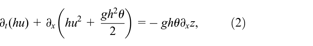
Here, we describe the properties of 1D and 2D Ripa models. The 1D Ripa model has the following form Chertock et al. ⁴

$${\partial }_{t}h+{\partial }_x(\mathrm{hu})=0,$$

(1)

$${\partial }_t(\mathrm{hu})+{\partial }_x(h{u}^2+\frac{g{h}^2\theta }{2})=-\mathrm{gh}\theta {\partial }_{x}z,$$

(2)

$${\partial }_t(h\theta )+{\partial }_x\left(\mathrm{hu}\theta \right)=0.$$

(3)

Where, $h(x,t)$ represents the water depth, $u(x,t)$ represents the fluid velocity in $x$ direction, $\theta$ is the temperature field, $z(x)$ denotes the bottom topography, and $g$ is the gravitational constant. The 1D Ripa model can be expressed as

$${\partial }_t\mathbf{U}+{\partial }_x\mathrm{F}(\mathbf{U})=\mathbf{Z}(\mathbf{U},x),$$

(4)

with $\mathbf{U}=(h,\mathrm{hu},h\theta )$ , $\mathbf{F}(\mathbf{U})=(F_1,F_2,F_3)=(\mathrm{hu},h{u}^2+\frac{g{h}^2\theta }{2},\mathrm{hu}\theta )$ , and $\mathbf{Z}(\mathbf{U},x)=(0,-\mathrm{gh}\theta {\partial }_{x}z,0).$ The eigen values of Jacobian matrix $\frac{\partial \mathbf{F}}{\partial \mathbf{U}}$ are ${\lambda }_1=u-\sqrt{\mathrm{gh}\theta },{\lambda }_2=u,{\lambda }_3=u+\sqrt{\mathrm{gh}\theta }$ . For the stability of proposed numerical schemes, these eigen values are used to find the dynamic time steps. Similar to the system of shallow water equations, the system (4) also has stationary solutions. These stationary solutions are well-explained in the articles.^5,41 One of them is described as

$$H=h+z=\mathrm{constant},u=0,\theta =\mathrm{constant}.$$

(5)

For this steady-state, the flux function is absolutely balanced by the source term.

The 2D Ripa model ⁴ is defined as

$${\partial }_{t}h+{\partial }_x(\mathrm{hu})+{\partial }_y(\mathrm{hv})=0,$$

(6)

$${\partial }_t(\mathrm{hu})+{\partial }_x(h{u}^2+\frac{g{h}^2\theta }{2})+{\partial }_y(\mathrm{huv})=-\mathrm{gh}\theta {\partial }_{x}z,$$

(7)

$${\partial }_t(\mathrm{hv})+{\partial }_x(\mathrm{huv})+{\partial }_y(h{v}^2+\frac{g{h}^2\theta }{2})=-\mathrm{gh}\theta {\partial }_{y}z,$$

(8)

$${\partial }_t(h\theta )+{\partial }_x\left(\mathrm{hu}\theta \right)+{\partial }_y\left(\mathrm{hv}\theta \right)=0.$$

(9)

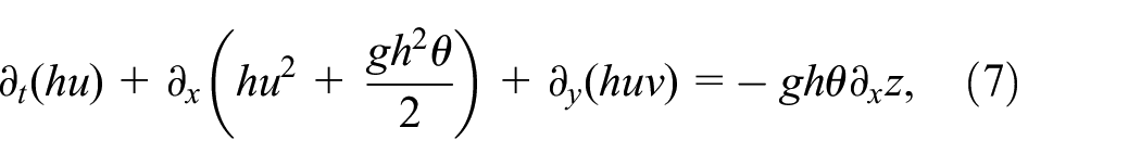
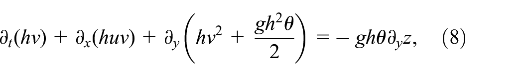
Here, $h(x,y,t)$ represents the water depth, $u(x,y,t)$ and $v(x,y,t)$ represent the fluid velocities in $x$ and $y$ directions respectively, $\theta$ is the temperature field, $z(x,y)$ denotes the bottom topography, and $g$ is the gravitational constant. The 2D Ripa model is written in compact form as

$${\partial }_t\mathbf{U}+{\partial }_x\mathbf{F}(\mathbf{U})+{\partial }_y\mathbf{G}(\mathbf{U})=\mathbf{Z}(\mathbf{U},\mathbf{X}),$$

(10)

with $\mathbf{U}=(h,\mathrm{hu},\mathrm{hv},h\theta )$ , $\mathbf{F}(\mathbf{U})=(F_1,F_2,F_3,F_4)=(\mathrm{hu},h{u}^2+\frac{g{h}^2\theta }{2},\mathrm{huv},\mathrm{hu}\theta )$ , $\mathbf{G}(\mathbf{U})=(\mathrm{hv},\mathrm{huv},h{v}^2+\frac{g{h}^2\theta }{2},\mathrm{hv}\theta )$ , and $\mathbf{Z}(\mathbf{U},\mathbf{X})=(0,-\mathrm{gh}\theta {\partial }_{x}z,-\mathrm{gh}\theta {\partial }_{y}z,0).$ The eigen values of Jacobian matrix $\frac{\partial F}{\partial \mathbf{U}}$ are ${\lambda }_1=u-\sqrt{\mathrm{gh}\theta },{\lambda }_2=u,{\lambda }_3=u,{\lambda }_4=u+\sqrt{\mathrm{gh}\theta }$ and the corresponding eigen values of the Jacobian matrix $\frac{\partial G}{\partial \mathbf{U}}$ are ${\sigma }_1=v-\sqrt{\mathrm{gh}\theta },{\sigma }_2=v,{\sigma }_3=v,{\sigma }_4=v+\sqrt{\mathrm{gh}\theta }$ .

The system (10) also admits stationary solutions in which flux gradients are balanced by the source terms in the steady state case. One of them is expressed as

$$H=h+z=\mathrm{Constant},\theta =\mathrm{Constant},u=0,v=0,$$

(11)

Similar to the 1D case, for the steady-state in equation (11), the source terms are completely balanced by the flux gradients in 2D Ripa model.

Construction of high order FV MR-WENO schemes for the Ripa models

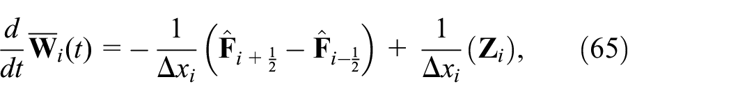
In this section, we construct FV MR-WENO numerical algorithm for computing the Ripa models. First, we consider the homogeneous form of the considered model (4) as follow

$${\partial }_t\mathbf{U}+{\partial }_x\mathbf{F}(\mathbf{U})=0,t>0,x\in \mathrm{\Omega },$$

(12)

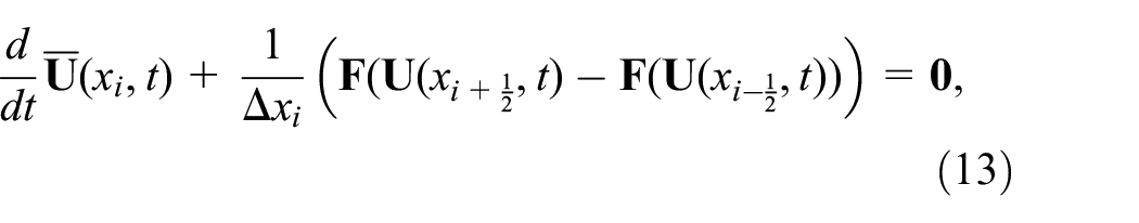
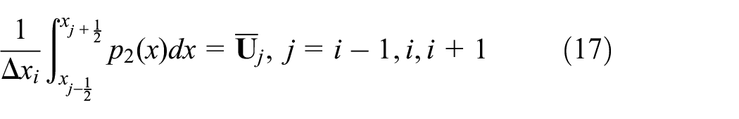
and divide the domain $\mathrm{\Omega }$ into cells $C_i=[x_{i-\frac{1}{2}},x_{i+\frac{1}{2}}],i=1,...,N.$ Here, the center of $i-\mathrm{th}$ cell is denoted by $x_i=\frac{(x_{i-\frac{1}{2}}+x_{i+\frac{1}{2}})}{2}$ and length of $i-\mathrm{th}$ cell by $\mathrm{\Delta }{x}_i.$ By integrating the equation (12) over $C_i$ , we have

$$\frac{d}{\mathrm{dt}}\overline{\mathbf{U}}(x_i,t)+\frac{1}{\mathrm{\Delta }{x}_i}(\mathbf{F}(\mathbf{U}(x_{i+\frac{1}{2}},t)-\mathbf{F}(\mathbf{U}(x_{i-\frac{1}{2}},t)))=0,$$

(13)

where $\overline{\mathbf{U}}(x_i,t)=\frac{1}{\mathrm{\Delta }{x}_i}{\int }_{x_{i-\frac{1}{2}}}^{x_{i+\frac{1}{2}}}\mathbf{U}(x,t)\mathrm{dx}$ . The equation (13) is approximated by the conservative scheme, as described in follow

$$\frac{d}{\mathrm{dt}}{\overline{\mathbf{U}}}_i(t)+\frac{1}{\mathrm{\Delta }{x}_i}({\hat{\mathbf{F}}}_{i+\frac{1}{2}}-{\hat{\mathbf{F}}}_{i-\frac{1}{2}})=0.$$

(14)

Where, ${\hat{\mathbf{F}}}_{i+\frac{1}{2}}=\mathsf{F}({\mathbf{U}}_{i+\frac{1}{2}}^{-},{\mathbf{U}}_{i+\frac{1}{2}}^{+})$ denotes the monotone numerical flux and ${\mathbf{U}}_{i+\frac{1}{2}}^{\pm }$ are pointwise approximations to $\mathbf{U}(x_{i+\frac{1}{2}},t)$ . Here, we will use the Lax-Friedrichs flux (LFF) as a monotone numerical flux which is defined as below

$$\begin{array}{c}\mathsf{F}({\mathbf{U}}_{i+\frac{1}{2}}^{-},{\mathbf{U}}_{i+\frac{1}{2}}^{+})\hfill \\ =\frac{1}{2}(\mathbf{F}({\mathbf{U}}_{i+\frac{1}{2}}^{-})+\mathbf{F}({\mathbf{U}}_{i+\frac{1}{2}}^{+})-\vartheta ({\mathbf{U}}_{i+\frac{1}{2}}^{+}-{\mathbf{U}}_{i+\frac{1}{2}}^{-})),\hfill \end{array}$$

(15)

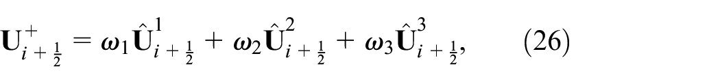
where $\vartheta =\underset{\mathbf{U}}{max}|\mathbf{F}\prime (\mathbf{U})|$ . Now computational variables are ${\overline{\mathbf{U}}}_i(t)$ which will approximate the cell-averages $\overline{\mathbf{U}}(x_i,t)$ . Further, the ${\mathbf{U}}_{i+\frac{1}{2}}^{-}$ and ${\mathbf{U}}_{i+\frac{1}{2}}^{+}$ are calculated through the adjacent cell-average values ${\overline{\mathbf{U}}}_i$ by MR-WENO reconstruction. For the fifth order MR-WENO reconstruction, we choose three central candidate stencils, ${\mathbb{S}}_1(i)=\{C_i\},{\mathbb{S}}_2(i)=\{C_{i-1},C_i,C_{i+1}\}$ and ${\mathbb{S}}_3(i)=\{C_{i-2},C_{i-1},C_i,C_{i+1},C_{i+2}\}$ and reconstruct the zeroth, second, and fourth degree polynomials $p_1(x),p_2(x)$ , and $p_3(x)$ respectively, which satisfy

$$\frac{1}{\mathrm{\Delta }{x}_i}{\int }_{x_{j-\frac{1}{2}}}^{x_{j+\frac{1}{2}}}{p}_1(x)\mathrm{dx}={\overline{\mathbf{U}}}_j,j=i,$$

(16)

$$\frac{1}{\mathrm{\Delta }{x}_i}{\int }_{x_{j-\frac{1}{2}}}^{x_{j+\frac{1}{2}}}{p}_2(x)\mathrm{dx}={\overline{\mathbf{U}}}_j,j=i-1,i,i+1$$

(17)

$$\frac{1}{\mathrm{\Delta }{x}_i}{\int }_{x_{j-\frac{1}{2}}}^{x_{j+\frac{1}{2}}}{p}_3(x)\mathrm{dx}={\overline{\mathbf{U}}}_j,j=i-2,i-1,i,i+1,i+2.$$

(18)

More precisely, the explicit expressions for $p_1(x),p_2(x)$ , and $p_3(x)$ are given as follow

$$p_1(x)={\overline{\mathbf{U}}}_i,$$

(19)

$$\begin{array}{c}\multicolumn{1}{c}{p_2(x)=\frac{{\overline{\mathbf{U}}}_{i+1}-2{\overline{\mathbf{U}}}_i+{\overline{\mathbf{U}}}_{i-1}}{2(\mathrm{\Delta }{x}_i{)}^2}(x-x_i{)}^2}\\ +\frac{{\overline{\mathbf{U}}}_{i+1}-{\overline{\mathbf{U}}}_{i-1}}{2(\mathrm{\Delta }{x}_i)}(x-x_i)\hfill \\ +\frac{-{\overline{\mathbf{U}}}_{i+1}+26{\overline{\mathbf{U}}}_i-{\overline{\mathbf{U}}}_{i-1}}{24},\hfill \end{array}$$

(20)

$$\begin{array}{c}{p}_3(x)=\frac{1}{1920}\hfill \\ [\frac{(80{\overline{\mathbf{U}}}_{i-2}-320{\overline{\mathbf{U}}}_{i-1}+480{\overline{\mathbf{U}}}_i-320{\overline{\mathbf{U}}}_{i+1}+80{\overline{\mathbf{U}}}_{i+2})}{{(\mathrm{\Delta }{x}_i)}^4}\hfill \\ (x-x_i{)}^4\hfill \end{array}$$

(21)

$$\begin{array}{c}+\frac{(160{\overline{\mathbf{U}}}_{i-2}-320{\overline{\mathbf{U}}}_{i-1}+320{\overline{\mathbf{U}}}_{i+1}-160{\overline{\mathbf{U}}}_{i+2})}{{(\mathrm{\Delta }{x}_i)}^3}\hfill \\ (x-x_i{)}^3\hfill \end{array}$$

(22)

$$\begin{array}{c}+\frac{(120{\overline{\mathbf{U}}}_{i-2}-1440{\overline{\mathbf{U}}}_{i-1}+2640{\overline{\mathbf{U}}}_i-1440{\overline{\mathbf{U}}}_{i+1}+120{\overline{\mathbf{U}}}_{i+2})}{{(\mathrm{\Delta }{x}_i)}^2}\hfill \\ (x-x_i{)}^2\hfill \end{array}$$

(23)

$$\begin{array}{c}+\frac{(200{\overline{\mathbf{U}}}_{i-2}-1360{\overline{\mathbf{U}}}_{i-1}+1360{\overline{\mathbf{U}}}_{i+1}-200{\overline{\mathbf{U}}}_{i+2})}{(\mathrm{\Delta }{x}_i)}\hfill \\ (x-x_i)\hfill \end{array}$$

(24)

$$+(9{\overline{\mathbf{U}}}_{i-2}-116{\overline{\mathbf{U}}}_{i-1}+2134{\overline{\mathbf{U}}}_i-116{\overline{\mathbf{U}}}_{i+1}+9{\overline{\mathbf{U}}}_{i+2})].$$

(25)

The point-wise reconstructed values ${\mathbf{U}}_{i+\frac{1}{2}}^{+}$ and ${\mathbf{U}}_{i+\frac{1}{2}}^{-}$ are obtained by the following relations

$${\mathbf{U}}_{i+\frac{1}{2}}^{+}={\omega }_1{\hat{\mathbf{U}}}_{i+\frac{1}{2}}^1+{\omega }_2{\hat{\mathbf{U}}}_{i+\frac{1}{2}}^2+{\omega }_3{\hat{\mathbf{U}}}_{i+\frac{1}{2}}^3,$$

(26)

$${\mathbf{U}}_{i+\frac{1}{2}}^{-}={\tilde{\omega }}_1{\tilde{\mathbf{U}}}_{i-\frac{1}{2}}^1+{\tilde{\omega }}_2{\tilde{\mathbf{U}}}_{i-\frac{1}{2}}^2+{\tilde{\omega }}_3{\tilde{\mathbf{U}}}_{i-\frac{1}{2}}^2,$$

(27)

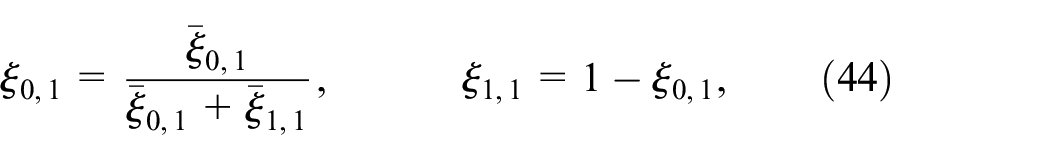
where ${\hat{\mathbf{U}}}_{i+\frac{1}{2}}^l$ and ${\tilde{\mathbf{U}}}_{i-\frac{1}{2}}^l$ , for $l=1,2,3$ , are reconstructed values. The values ${\tilde{\mathbf{U}}}_{i-\frac{1}{2}}^l$ are mirror symmetric to the values ${\hat{\mathbf{U}}}_{i+\frac{1}{2}}^l$ . Hence, we just define the values ${\hat{\mathbf{U}}}_{i+\frac{1}{2}}^l$ as follow

$${\hat{\mathbf{U}}}_{i+\frac{1}{2}}^1=p_1(x_{i+\frac{1}{2}}),$$

(28)

$${\hat{\mathbf{U}}}_{i+\frac{1}{2}}^2=\frac{1}{{\xi }_{2,2}}{p}_2(x_{i+\frac{1}{2}})-\frac{{\xi }_{1,2}}{{\xi }_{2,2}}{\hat{\mathbf{U}}}_{i+\frac{1}{2}}^1,$$

(29)

$${\hat{\mathbf{U}}}_{i+\frac{1}{2}}^3=\frac{1}{{\xi }_{3,3}}{p}_3(x_{i+\frac{1}{2}})-\frac{{\xi }_{1,3}}{{\xi }_{3,3}}{\hat{\mathbf{U}}}_{i+\frac{1}{2}}^1-\frac{{\xi }_{2,3}}{{\xi }_{3,3}}{\hat{\mathbf{U}}}_{i+\frac{1}{2}}^2,$$

(30)

with

$$p_1(x_{i+\frac{1}{2}})={\overline{\mathbf{U}}}_i,$$

(31)

$$p_2(x_{i+\frac{1}{2}})=\frac{-1}{6}{\overline{\mathbf{U}}}_{i-1}+\frac{5}{6}{\overline{\mathbf{U}}}_i+\frac{1}{3}{\overline{\mathbf{U}}}_{i+1},$$

(32)

$$\begin{array}{c}\multicolumn{1}{c}{p_3(x_{i+\frac{1}{2}})=\frac{1}{30}{\overline{\mathbf{U}}}_{i-2}-\frac{13}{60}{\overline{\mathbf{U}}}_{i-1}+\frac{47}{60}{\overline{\mathbf{U}}}_i}\\ +\frac{9}{20}{\overline{\mathbf{U}}}_{i+1}+\frac{1}{20}{\overline{\mathbf{U}}}_{i+2}.\hfill \end{array}$$

(33)

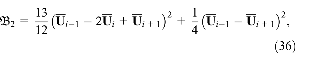
Where ${\xi }_{1,2}+{\xi }_{2,2}=1$ , ${\xi }_{1,3}+{\xi }_{2,3}+{\xi }_{3,3}=1$ , and ${\xi }_{2,2}$ , ${\xi }_{3,3}\ne 0$ . In these expressions, ${\xi }_{1,2},{\xi }_{2,2}$ are the linear weights. For a balance between the sharp and essentially non-oscillatory shock transitions in non-smooth regions and accuracy in smooth regions, we set the linear weights as ${\xi }_{1,2}=1/11$ , ${\xi }_{2,2}=10/11$ , ${\xi }_{1,3}=1/111$ , ${\xi }_{2,3}=10/111$ , and ${\xi }_{3,3}=100/111$ for the fifth-order approximation, as described in Zhu and Shu. ³⁴

The nonlinear weights ${\omega }_l$ in equation (26) are defined as

$$\begin{array}{c}{\omega }_l=\frac{{\overline{\omega }}_l}{\sum _{l=1}^m{\overline{\omega }}_l},{\overline{\omega }}_l={\xi }_{l,m}(1+\frac{\tau }{\epsilon +{\mathfrak{B}}_l}),\hfill \\ l=1,...,m;m=3.\hfill \end{array}$$

(34)

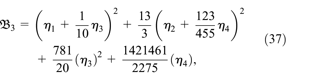
Here $\epsilon$ is taken as ${10}^{-10}$ in all the simulations. Here, ${\xi }_l$ and ${\mathfrak{B}}_l$ respectively denote the linear weights and smoothness indicators. These smoothness indicators in general form are written as

$${\mathfrak{B}}_m=\sum _{j=1}^{2(m-1)}{\int }_{x_{i-\frac{1}{2}}}^{x_{i+\frac{1}{2}}}{h}^{2j-1}{\left(\frac{d^j{p}_m(x)}{d{x}^j}\right)}^2\mathrm{dx},m=2,3,$$

(35)

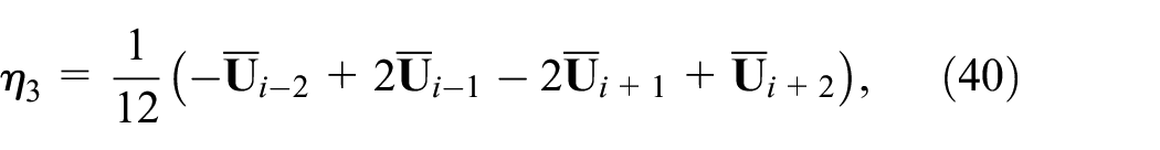
Here, the values of ${\mathfrak{B}}_1,{\mathfrak{B}}_2$ , and ${\mathfrak{B}}_3$ are defined in the same way as described in Shu^26,27 and Zhu and Shu. ³⁴ More precisely, these smooth indicators are defined as follow

$${\mathfrak{B}}_2=\frac{13}{12}{({\overline{\mathbf{U}}}_{i-1}-2{\overline{\mathbf{U}}}_i+{\overline{\mathbf{U}}}_{i+1})}^2+\frac{1}{4}{({\overline{\mathbf{U}}}_{i-1}-{\overline{\mathbf{U}}}_{i+1})}^2,$$

(36)

$$\begin{array}{c}\multicolumn{1}{c}{{\mathfrak{B}}_3={({\eta }_1+\frac{1}{10}{\eta }_3)}^2+\frac{13}{3}{({\eta }_2+\frac{123}{455}{\eta }_4)}^2}\\ +\frac{781}{20}{\left({\eta }_3\right)}^2+\frac{1421461}{2275}\left({\eta }_4\right),\hfill \end{array}$$

(37)

where

$${\eta }_1=\frac{1}{120}(11{\overline{\mathbf{U}}}_{i-2}-82{\overline{\mathbf{U}}}_{i-1}+82{\overline{\mathbf{U}}}_{i+1}-11{\overline{\mathbf{U}}}_{i+2}),$$

(38)

$${\eta }_2=\frac{1}{56}(-3{\overline{\mathbf{U}}}_{i-2}+40{\overline{\mathbf{U}}}_{i-1}-74{\overline{\mathbf{U}}}_{i+1}+40{\overline{\mathbf{U}}}_{i+1}-3{\overline{\mathbf{U}}}_{i+2}),$$

(39)

$${\eta }_3=\frac{1}{12}(-{\overline{\mathbf{U}}}_{i-2}+2{\overline{\mathbf{U}}}_{i-1}-2{\overline{\mathbf{U}}}_{i+1}+{\overline{\mathbf{U}}}_{i+2}),$$

(40)

$${\eta }_4=\frac{1}{24}({\overline{\mathbf{U}}}_{i-2}-4{\overline{\mathbf{U}}}_{i-1}+6{\overline{\mathbf{U}}}_i-4{\overline{\mathbf{U}}}_{i+1}+{\overline{\mathbf{U}}}_{i+2}).$$

(41)

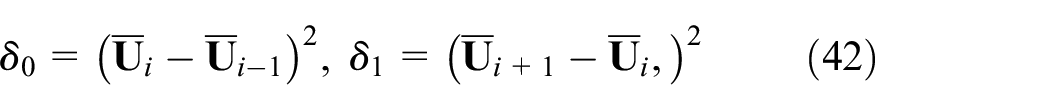
Now for resolving the discontinuities efficiently, the expression of ${\mathfrak{B}}_1$ is defined as follow

$${\delta }_0={({\overline{\mathbf{U}}}_i-{\overline{\mathbf{U}}}_{i-1})}^2,{\delta }_1={({\overline{\mathbf{U}}}_{i+1}-{\overline{\mathbf{U}}}_i,)}^2$$

(42)

$${\overline{\xi }}_{0,1}=\{\begin{array}{cc}1,\hfill & {\delta }_0>{\delta }_1,\hfill \\ \multicolumn{1}{c}{10,}& \mathrm{otherwise}\hfill \end{array},{\overline{\xi }}_{1,1}=1-{\overline{\xi }}_{0,1},$$

(43)

$${\xi }_{0,1}=\frac{{\overline{\xi }}_{0,1}}{{\overline{\xi }}_{0,1}+{\overline{\xi }}_{1,1}},{\xi }_{1,1}=1-{\xi }_{0,1},$$

(44)

$$\begin{array}{c}{\sigma }_0={\xi }_{0,1}(1+\frac{{|{\delta }_0-{\delta }_1|}^2}{{\delta }_0+\epsilon }),\hfill \\ {\sigma }_1={\xi }_{1,1}(1+\frac{{|{\delta }_0-{\delta }_1|}^2}{{\delta }_1+\epsilon }),\sigma ={\sigma }_0+{\sigma }_1.\hfill \end{array}$$

(45)

In equation (45), $\epsilon$ can be taken any small positive number for avoiding the denominator to become zero. In the last, we set

$${\mathfrak{B}}_1=\frac{1}{{\sigma }^2}({\sigma }_0({\overline{\mathbf{U}}}_i-{\overline{\mathbf{U}}}_{i-1})+{\sigma }_1({\overline{\mathbf{U}}}_{i+1}-{\overline{\mathbf{U}}}_i)).$$

(46)

The term $\tau$ in equation (34) is given as

$$\tau =\left(\frac{\sum _{l=1}^2|{\mathfrak{B}}_3-{\mathfrak{B}}_l|}{2}\right).$$

(47)

This completes the procedure of spatial reconstruction.

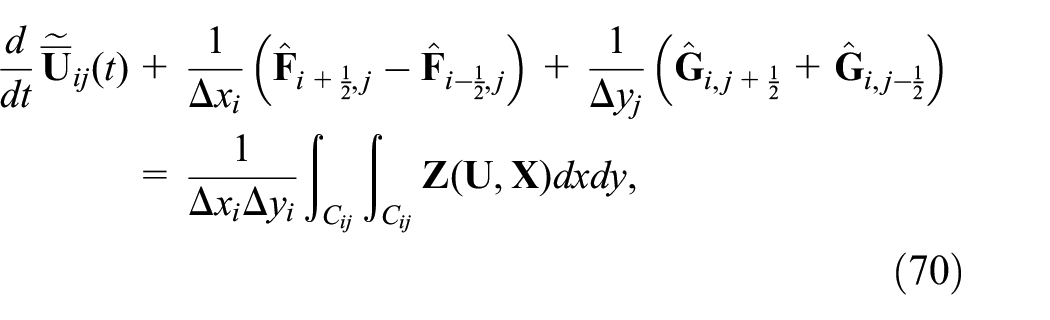
Next we describe the finite volume MR-WENO scheme for 2D Ripa model. Consider the two-dimensional Ripa model (10) in homogeneous form as follow

$${\partial }_t\mathbf{U}+{\partial }_{x}F(\mathbf{U})+{\partial }_{y}G(\mathbf{U})=0,t>0,x,y\in \mathrm{\Omega }.$$

(48)

Divide the computational domain $\mathrm{\Omega }$ into cells $C_{\mathrm{ij}}=[x_{i-\frac{1}{2}},x_{i+\frac{1}{2}}]\times [y_{j-\frac{1}{2}},y_{j+\frac{1}{2}}],i=1,...,N_x,j=1,...,N_y.$ and integrate the equation (48) over cell $C_{\mathrm{ij}}$ to obtain

$$\begin{array}{c}\frac{d}{\mathrm{dt}}\widetilde{\overline{\mathbf{U}}}(x_i,y_j,t)+\frac{1}{\mathrm{\Delta }{x}_i\mathrm{\Delta }{y}_j}\hfill \\ ({\int }_{y_{j-\frac{1}{2}}}^{y_{j+\frac{1}{2}}}F(\mathbf{U}(x_{i+\frac{1}{2}},y,t))\mathrm{dy}-{\int }_{y_{j-\frac{1}{2}}}^{y_{j+\frac{1}{2}}}F(\mathbf{U}(x_{i-\frac{1}{2}},y,t))\mathrm{dy}\hfill \\ +{\int }_{y_{j-\frac{1}{2}}}^{y_{j+\frac{1}{2}}}G(\mathbf{U}(x,y_{j+\frac{1}{2}},t))\mathrm{dy}-{\int }_{y_{j-\frac{1}{2}}}^{y_{j+\frac{1}{2}}}G(\mathbf{U}(x,y_{j-\frac{1}{2}},t))\mathrm{dy})=0,\hfill \end{array}$$

(49)

where $\widetilde{\overline{\mathbf{U}}}(x_i,y_i,t)=\frac{1}{\mathrm{\Delta }{x}_i\mathrm{\Delta }{y}_j}{\int }_{y_{j-\frac{1}{2}}}^{y_{j+\frac{1}{2}}}{\int }_{x_{i-\frac{1}{2}}}^{x_{i+\frac{1}{2}}}\mathbf{U}(x,y,t)\mathrm{dxdy}$ is the cell average. The notations $\widetilde{(·)}$ and $\overline{(·)}$ denote the cell average in $x$ -direction and cell average in $y$ -direction. The equation (49) is approximated as follow

$$\begin{array}{c}\multicolumn{1}{c}{\frac{d}{\mathrm{dt}}{\widetilde{\overline{\mathbf{U}}}}_{\mathrm{ij}}(t)+\frac{1}{\mathrm{\Delta }{x}_i}({\hat{F}}_{i+\frac{1}{2},j}-{\hat{F}}_{i-\frac{1}{2},j})}\\ +\frac{1}{\mathrm{\Delta }{y}_j}({\hat{G}}_{i,j+\frac{1}{2}}-{\hat{G}}_{i,j-\frac{1}{2}})=0,\hfill \end{array}$$

(50)

where numerical fluxes are defined as

$${\hat{F}}_{i+\frac{1}{2},j}=\sum _{l=1}^3{\Upsilon }_l\hat{F}({\mathbf{U}}_{i+\frac{1}{2},j+{\phi }_l}^{-},{\mathbf{U}}_{i+\frac{1}{2},j+{\phi }_l}^{+})={\tilde{F}}_{i+\frac{1}{2},j},$$

(51)

and

$${\hat{G}}_{i,j+\frac{1}{2}}=\sum _{l=1}^3{\Upsilon }_l\hat{G}({\mathbf{U}}_{i+{\phi }_l,j+\frac{1}{2}}^{-},{\mathbf{U}}_{i+{\phi }_l,j+\frac{1}{2}}^{+})={\overline{G}}_{i,j+\frac{1}{2}},$$

(52)

with ${\hat{F}}_{i+\frac{1}{2},j}=\mathsf{F}({\mathbf{U}}_{i+\frac{1}{2},j+{\phi }_l}^{-},{\mathbf{U}}_{i+\frac{1}{2},j+{\phi }_l}^{+})$ and ${\hat{G}}_{i+{\phi }_l,j+\frac{1}{2}}=\mathsf{F}({\mathbf{U}}_{i+{\phi }_l,j+\frac{1}{2}}^{-},{\mathbf{U}}_{i,j+\frac{1}{2}}^{+})$ , where numerical flux $\mathsf{F}(a,b)$ is defined on the same lines as given in equation (15) and ${\mathbf{U}}_{i+\frac{1}{2},j+{\phi }_l}^{\pm }$ and ${\mathbf{U}}_{i+{\phi }_l,j+\frac{1}{2}}^{\pm }$ are approximations acquired by MR-WENO reconstruction strategy in a dimension-by-dimension way. ${\Upsilon }_l$ and ${\phi }_l$ are the Gaussian quadrature weights and nodes. Here, for the fifth order reconstruction, we varies $l$ from $1$ to $3$ . For more detail about the implementation of two dimensional WENO schemes, the reader is referred to Shu^26,27 and Zhu and Shu. ³⁴

Construction of well-balanced techniques for the Ripa systems

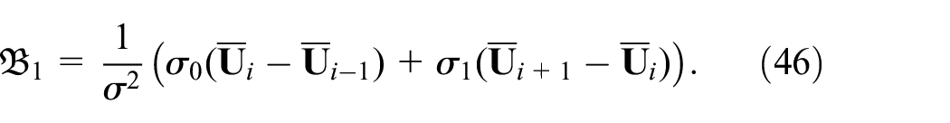
Here, we construct a high order well-balanced FV MR-WENO scheme for 1D and 2D Ripa models. First we construct a well-balanced high order finite volume WENO scheme for 1D Ripa model (4). By using equations (4) and (14), we obtain the semi-discrete form of 1D Ripa model as follow

$$\frac{d}{\mathrm{dt}}{\overline{\mathbf{U}}}_i(t)=-\frac{1}{\mathrm{\Delta }{x}_i}({\hat{\mathbf{F}}}_{i+\frac{1}{2}}-{\hat{\mathbf{F}}}_{i-\frac{1}{2}})+\frac{1}{\mathrm{\Delta }{x}_i}{\int }_{C_i}\mathbf{Z}(\mathbf{U},x)\mathrm{dx},$$

(53)

The key idea to develop a well-balanced FV MR-WENO scheme which exactly preserves the steady-states (5) is to decompose the integral of non-conservative term in equation (53) into sum of various terms. Each term is computed in a way that consistent with the corresponding computed flux terms. The first step in construction of high order well-balanced FV MR-WENO method is to obtain the values of ${\mathbf{U}}_{i+\frac{1}{2}}^{\pm }$ from the given cell averages ${\overline{\mathbf{U}}}_i$ as explained in Section 3. Consider that the source term can be written as

$$\mathbf{Z}(\mathbf{U},x)=Z_q(\mathbf{U},x)=\sum _r{s}_r(a_r(\mathbf{U},x))b_r^{\prime }(x),q=1,2,3,$$

(54)

where $s_r$ and $b_r$ are some known functions, for more detail, see Xing and Shu. ³³ Since the source term of Ripa model is

$$\mathbf{Z}(\mathbf{U},x)=(Z_1(\mathbf{U},x),Z_2(\mathbf{U},x),Z_3(\mathbf{U},x)=(0,-\mathrm{gh}\theta {\partial }_{x}z,0)).$$

(55)

As $Z_1(\mathbf{U},x)$ and $Z_3(\mathbf{U},x)$ are zeros so only $Z_2(\mathbf{U},x)$ is written as

$$Z_2(\mathbf{U},x)=-\mathrm{gh}\theta {\partial }_{x}z=-g\theta (h+z)z_x+\frac{g\theta }{2}(z^2{)}_x.$$

(56)

From equations (5), (54), and (56), we have

$$\begin{array}{c}{a}_1=z+h=\mathrm{constant},a_2=u=0,a_3=\theta ,\hfill \\ \multicolumn{1}{c}{s_1(a_1)=-g\theta (h+z),s_2(a_2)=\frac{g\theta }{2},}\\ \multicolumn{1}{c}{b_1(x)=z,b_2(x)=z^2.}\end{array}$$

(57)

For the construction of high order finite volume scheme apply MR-WENO reconstruction to the function $(0,z(x),0)$ , with coefficients computed from $h,\mathrm{hu},h\theta$ , to obtain $z_{i+\frac{1}{2}}^{\pm }$ . Next integrate the source term in equation (54) over the cell $C_i$ as

$${\int }_{C_i}\mathbf{Z}(\mathbf{U},x)\mathrm{dx}=\sum _r{\int }_{C_i}{s}_r(a_r(\mathbf{U},x))b_r^{\prime }(x)\mathrm{dx}.$$

(58)

and decompose it in the following way

$$\begin{array}{c}\sum _r{\int }_{C_i}{s}_r(a_r(\mathbf{U},x))b_r^{\prime }(x)\mathrm{dx}\hfill \\ =\sum _r(\frac{1}{2}(s_r(a_r(\mathbf{U},x{)}_{i-\frac{1}{2}}^{+})+s_r(a_r(\mathbf{U},x{)}_{i+\frac{1}{2}}^{-})){\int }_{C_i}{b}_r^{\prime }(x)\mathrm{dx}\hfill \\ +{\int }_{C_i}(s_r(a_r(\mathbf{U},x))-\frac{1}{2}(s_r(a_r(\mathbf{U},x{)}_{i-\frac{1}{2}}^{+})+s_r(a_r(\mathbf{U},x{)}_{i+\frac{1}{2}}^{-})))b_r^{\prime }(x)\mathrm{dx})\hfill \\ =\sum _r(\frac{1}{2}(s_r(a_r(\mathbf{U},x{)}_{i-\frac{1}{2}}^{+})+s_r(a_r(\mathbf{U},x{)}_{i+\frac{1}{2}}^{-}))(b_r(x_{i+\frac{1}{2}})-b_r(x_{i-\frac{1}{2}}))\hfill \\ +{\int }_{C_i}(s_r(a_r(\mathbf{U},x))-\frac{1}{2}(s_r(a_r(\mathbf{U},x{)}_{i-\frac{1}{2}}^{+})+s_r(a_r(\mathbf{U},x{)}_{i+\frac{1}{2}}^{-})))b_r^{\prime }(x)\mathrm{dx}),\hfill \end{array}$$

(59)

The high order approximations $(b_r{)}_{i+\frac{1}{2}}^{\pm }$ to $b_r(x_{i+\frac{1}{2}})$ are chosen suitably which satisfy the following relation

$$F_2({\mathbf{U}}_{i+\frac{1}{2}}^{\pm })-\sum _r{s}_r(a_r(\mathbf{U},x{)}_{i+\frac{1}{2}}^{\pm }(b_r{)}_{i+\frac{1}{2}}^{\pm })=\mathrm{constant},$$

(60)

when the steady-state is reached. For 1D Ripa model these high order approximations $(b_r{)}_{i+\frac{1}{2}}^{\pm }$ are defined as

$$(b_1{)}_{i+\frac{1}{2}}^{\pm }=z_{i+\frac{1}{2}}^{\pm },(b_2{)}_{i+\frac{1}{2}}^{\pm }=(z_{i+\frac{1}{2}}^{\pm }{)}^2.$$

(61)

and clearly for the steady-state (11) and (57), we have

$$\begin{array}{c}{F}_2(U_{i+\frac{1}{2}}^{+})-\sum _r{s}_r(a_r(U,x{)}_{i+\frac{1}{2}}^{+}(b_r{)}_{i+\frac{1}{2}}^{+}\hfill \\ =\frac{g}{2}({\theta }_{i+\frac{1}{2}}^{+})(h_{i+\frac{1}{2}}^{+}{)}^2+\frac{g}{2}({\theta }_{i+\frac{1}{2}}^{-}(h_{i+\frac{1}{2}}^{-}+z_{i+\frac{1}{2}}^{-})\hfill \\ +{\theta }_{i+\frac{1}{2}}^{+}(h_{i+\frac{1}{2}}^{+}+z_{i+\frac{1}{2}}^{+}))z_{i+\frac{1}{2}}^{+}-\frac{g}{2}{\theta }_{i+\frac{1}{2}}^{+}(z_{i+\frac{1}{2}}^{+}{)}^2\hfill \\ =\frac{g}{2}(\mathrm{c})((h_{i+\frac{1}{2}}^{+}{)}^2-(z_{i+\frac{1}{2}}^{+}{)}^2)+g(\mathrm{c})(\mathrm{c})z_{i+\frac{1}{2}}^{+}\hfill \\ =\frac{g}{2}(\mathrm{c})((h_{i+\frac{1}{2}}^{+})+(z_{i+\frac{1}{2}}^{+}))((h_{i+\frac{1}{2}}^{+})-(z_{i+\frac{1}{2}}^{+}))+g(\mathrm{c})(\mathrm{c})z_{i+\frac{1}{2}}^{+}\hfill \\ =\frac{g}{2}(\mathrm{c})(\mathrm{c})((h_{i+\frac{1}{2}}^{+})-(z_{i+\frac{1}{2}}^{+}))+g(\mathrm{c})(\mathrm{c})z_{i+\frac{1}{2}}^{+}\hfill \\ =\frac{g}{2}(\mathrm{c}{)}^2((h_{i+\frac{1}{2}}^{+})-(z_{i+\frac{1}{2}}^{+})+2(z_{i+\frac{1}{2}}^{+}))\hfill \\ =\frac{g}{2}(\mathrm{c}{)}^3.\hfill \end{array}$$

Similarly we can get $F_2({\mathbf{U}}_{i+\frac{1}{2}}^{-})-\sum _r{s}_r(a_r(\mathbf{U},x{)}_{i+\frac{1}{2}}^{-}(b_r{)}_{i+\frac{1}{2}}^{-}=\frac{g}{2}(\mathrm{c}{)}^3.$ Thus the source term takes the following form

$$\begin{array}{c}\sum _r{\int }_{C_i}{s}_r(a_r(\mathbf{U},x))b_r^{\prime }(x)\mathrm{dx}\hfill \\ =\sum _r(\frac{1}{2}(s_r(a_r(\mathbf{U},x{)}_{i-\frac{1}{2}}^{+})+s_r(a_r(\mathbf{U},x{)}_{i+\frac{1}{2}}^{-}))(({\hat{b}}_r{)}_{i+\frac{1}{2}}-({\hat{b}}_r{)}_{i-\frac{1}{2}})\hfill \\ +{\int }_{C_i}(s_r(a_r(\mathbf{U},x))-\frac{1}{2}(s_r(a_r(\mathbf{U},x{)}_{i-\frac{1}{2}}^{+})+s_r(a_r(\mathbf{U},x{)}_{i+\frac{1}{2}}^{-})))b_r^{\prime }(x)\mathrm{dx}),\hfill \end{array}$$

(62)

where $({\hat{b}}_r{)}_{i+\frac{1}{2}}$ is approximation to $b_r(x_{i+\frac{1}{2}})$ and defined as

$$({\hat{b}}_r{)}_{i+\frac{1}{2}}=\frac{((b_r{)}_{i+\frac{1}{2}}^{-}+(b_r{)}_{i+\frac{1}{2}}^{+})}{2}.$$

(63)

The remaining integral term in equation (62) is computed by high order Gauss-Lobatto quadrature. Finally, for the construction of well-balanced FV MR-WENO scheme, introduced a minor change in a monotone Lax-Friedrichs numerical flux

$$\begin{array}{c}\multicolumn{1}{c}{{\hat{\mathbf{F}}}_{i+\frac{1}{2}}=\mathsf{F}({\mathbf{U}}_{i+\frac{1}{2}}^{-},{\mathbf{U}}_{i+\frac{1}{2}}^{+})}\\ =\frac{1}{2}[\mathbf{F}({\mathbf{U}}_{i+\frac{1}{2}}^{-})+\mathbf{F}({\mathbf{U}}_{i+\frac{1}{2}}^{+})-\vartheta ({\mathbf{U}}_{i+\frac{1}{2}}^{+}-{\mathbf{U}}_{i+\frac{1}{2}}^{-})],\hfill \end{array}$$

by replacing $({\mathbf{U}}_{i+\frac{1}{2}}^{+}-{\mathbf{U}}_{i+\frac{1}{2}}^{-})$ with $(\mathbf{a}(\mathbf{U},x{)}_{i+\frac{1}{2}}^{+}-\mathbf{a}(\mathbf{U},x{)}_{i+\frac{1}{2}}^{-})$ , where $\mathbf{a}(\mathbf{U},x{)}_{i+\frac{1}{2}}^{+}=(a_1(\mathbf{U},x{)}_{i+\frac{1}{2}}^{+},a_2(\mathbf{U},x{)}_{i+\frac{1}{2}}^{+},a_3(\mathbf{U},x{)}_{i+\frac{1}{2}}^{+})$ . Now modified numerical flux becomes

$$\begin{array}{c}\multicolumn{1}{c}{{\hat{\mathbf{F}}}_{i+\frac{1}{2}}=\mathsf{F}({\mathbf{U}}_{i+\frac{1}{2}}^{-},{\mathbf{U}}_{i+\frac{1}{2}}^{+})}\\ =\frac{1}{2}[\mathbf{F}({\mathbf{U}}_{i+\frac{1}{2}}^{-})+\mathbf{F}({\mathbf{U}}_{i+\frac{1}{2}}^{+})-\vartheta (\mathbf{a}(\mathbf{U},x{)}_{i+\frac{1}{2}}^{+}-\mathbf{a}(\mathbf{U},x{)}_{i+\frac{1}{2}}^{-}].\hfill \end{array}$$

(64)

This completes the construction of well-balanced FV MR-WENO scheme for 1D Ripa system. Finally, we end up with the semi-discrete equation as follow

$$\frac{d}{\mathrm{dt}}{\overline{\mathbf{W}}}_i(t)=-\frac{1}{\mathrm{\Delta }{x}_i}({\hat{\mathbf{F}}}_{i+\frac{1}{2}}-{\hat{\mathbf{F}}}_{i-\frac{1}{2}})+\frac{1}{\mathrm{\Delta }{x}_i}\left({\mathbf{Z}}_i\right),$$

(65)

or the above equation can be described as

$$\frac{d}{\mathrm{dt}}{\overline{\mathbf{W}}}_i(t)=\mathcal{L}(\mathbf{W}).$$

(66)

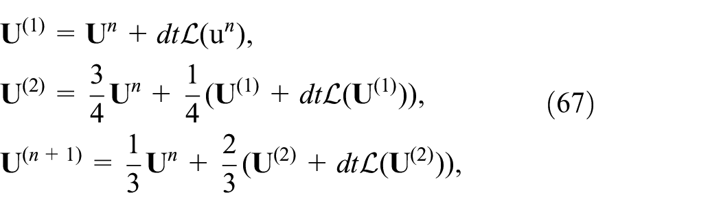
Where $\mathcal{L}(\mathrm{u})$ denotes spatial operator. Now, for solving the system of ordinary differential equations (66), we apply the third order TVD RK method ¹⁶ as follow

$$\begin{array}{c}{\mathbf{U}}^{(1)}={\mathbf{U}}^n+\mathrm{dt}\mathcal{L}({\mathrm{u}}^n),\hfill \\ {\mathbf{U}}^{(2)}=\frac{3}{4}{\mathbf{U}}^n+\frac{1}{4}({\mathbf{U}}^{(1)}+\mathrm{dt}\mathcal{L}({\mathbf{U}}^{(1)})),\hfill \\ {\mathbf{U}}^{(n+1)}=\frac{1}{3}{\mathbf{U}}^n+\frac{2}{3}({\mathbf{U}}^{(2)}+\mathrm{dt}\mathcal{L}({\mathbf{U}}^{(2)})),\hfill \end{array}$$

(67)

with $\mathrm{dt}=\frac{\mathrm{CFL}·\mathrm{dx}}{\vartheta }$ where $\vartheta =\mathrm{ma}{x}_{\mathbf{U}}|\lambda (\mathbf{U})|$ and CFL denotes Courant-Friedrichs-Lewy coefficient.

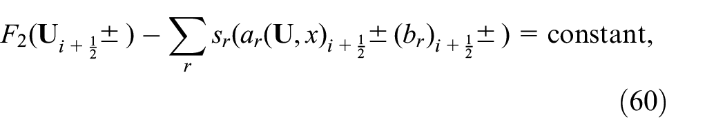
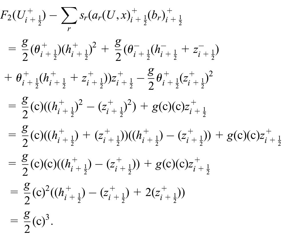
• Proposition 4.1. The construction of FV MR-WENO method with modified Lax-Friedrichs numerical flux is a well-balanced scheme and high order accurate for general solutions.

Proof. Obviously, for the steady-state solution, $a_r(\mathbf{U},x)$ and $a_r(\mathbf{U},x{)}_{i\pm \frac{1}{2}}^{\pm }$ are equal to the same constant $c$ at each Gauss-Lobatto point in equation (59), so the integral term

$${\int }_{C_i}(s_r(a_r(\mathbf{U},x))-\frac{1}{2}(s_r(a_r(\mathbf{U},x{)}_{i-\frac{1}{2}}^{+})+s_r(a_r(\mathbf{U},x{)}_{i+\frac{1}{2}}^{-})))b_r^{\prime }(x)\mathrm{dx},$$

becomes zero and flux term in equation (64) becomes

$${\hat{\mathbf{F}}}_{i+\frac{1}{2}}=\frac{1}{2}[\mathbf{F}({\mathbf{U}}_{i+\frac{1}{2}}^{-})+\mathbf{F}({\mathbf{U}}_{i+\frac{1}{2}}^{+})].$$

(68)

Now the truncation error term reduces to

$$\begin{array}{c}-{\hat{F}}_{2,i+\frac{1}{2}}+{\hat{F}}_{2,i-\frac{1}{2}}+\sum _r(\frac{1}{2}(s_r(a_r(\mathbf{U},x{)}_{i-\frac{1}{2}}^{+})+s_r(a_r(\mathbf{U},x{)}_{i+\frac{1}{2}}^{-}))(({\hat{b}}_r{)}_{i+\frac{1}{2}}-({\hat{b}}_r{)}_{i-\frac{1}{2}}),\hfill \\ =-{\hat{F}}_{2,i+\frac{1}{2}}+{\hat{F}}_{2,i-\frac{1}{2}}+\sum _r(s_r(c))(({\hat{b}}_r{)}_{i+\frac{1}{2}}-({\hat{b}}_r{)}_{i-\frac{1}{2}}),\hfill \\ =-{\hat{F}}_{2,i+\frac{1}{2}}+\sum _r(s_r(\mathrm{c}))(({\hat{b}}_r{)}_{i+\frac{1}{2}})+{\hat{F}}_{2,i-\frac{1}{2}}-\sum _r(s_r(\mathrm{c}))(({\hat{b}}_r{)}_{i-\frac{1}{2}}),\hfill \\ =-\frac{1}{2}({\hat{F}}_2({\mathbf{U}}_{i+\frac{1}{2}}^{-})+{\hat{F}}_2({\mathbf{U}}_{i+\frac{1}{2}}^{+}))+\sum _r(s_r(c))\frac{1}{2}((b_r{)}_{i+\frac{1}{2}}^{+}+(b_r{)}_{i+\frac{1}{2}}^{-})\hfill \\ +\frac{1}{2}({\hat{F}}_2({\mathbf{U}}_{i-\frac{1}{2}}^{-})+{\hat{F}}_2({\mathbf{U}}_{i-\frac{1}{2}}^{+}))-\sum _r(s_r(c)))\frac{1}{2}((b_r{)}_{i-\frac{1}{2}}^{+}+(b_r{)}_{i-\frac{1}{2}}^{-}),\hfill \end{array}$$

(69)

By using equation (60), the expression in equation (69) becomes zero which shows that the proposed numerical scheme is well-balanced. It is straightforward that the proposed numerical scheme is high order accurate for general solutions.

Now we explain the construction of well-balanced finite volume scheme for 2D Ripa model. By using the equations (10) and (50) with equations (51) and (52), semidiscrete form of the 2D Ripa model is written as

$$\begin{array}{c}\multicolumn{1}{c}{\frac{d}{\mathrm{dt}}{\widetilde{\overline{\mathbf{U}}}}_{\mathrm{ij}}(t)+\frac{1}{\mathrm{\Delta }{x}_i}({\hat{\mathbf{F}}}_{i+\frac{1}{2},j}-{\hat{\mathbf{F}}}_{i-\frac{1}{2},j})+\frac{1}{\mathrm{\Delta }{y}_j}({\hat{\mathbf{G}}}_{i,j+\frac{1}{2}}+{\hat{\mathbf{G}}}_{i,j-\frac{1}{2}})}\\ =\frac{1}{\mathrm{\Delta }{x}_i\mathrm{\Delta }{y}_i}{\int }_{C_{\mathrm{ij}}}{\int }_{C_{\mathrm{ij}}}\mathbf{Z}(\mathbf{U},\mathbf{X})\mathrm{dxdy},\hfill \end{array}$$

(70)

where the source term of 2D Ripa model is

$$\begin{array}{c}\multicolumn{1}{c}{\mathbf{Z}(\mathbf{U},\mathbf{X})=(Z_1(\mathbf{U},x,y),Z_2(\mathbf{U},x,y),Z_3(\mathbf{U},x,y),}\\ Z_4(\mathbf{U},x,y)=(0,-\mathrm{gh}\theta {\partial }_{x}z,-\mathrm{gh}\theta {\partial }_{y}z,0)).\hfill \end{array}$$

(71)

As $Z_1(\mathbf{U},x,y)$ and $Z_4(\mathbf{U},x,y)$ are zeros, so the decomposition of $Z_2(\mathbf{U},x,y)$ and $Z_3(\mathbf{U},x,y)$ is written as

$$Z_2(\mathbf{U},x)=-\mathrm{gh}\theta {\partial }_{x}z=-g\theta (h+z)z_x+\frac{g\theta }{2}(z^2{)}_x,$$

(72)

and

$$Z_3(\mathbf{U},x)=-\mathrm{gh}\theta {\partial }_{y}z=-g\theta (h+z)z_y+\frac{g\theta }{2}(z^2{)}_y.$$

(73)

Next we follow the same procedure in each of the $x$ and $y$ directions as discussed for the construction of 1D case.

Central upwind numerical scheme

For validation and checking the accuracy, the results obtained from the multi-resolution WENO numerical schemes are compared with the results obtained from the CUP schemes. ⁴⁰ Here, only final formulaton of the second order CUP scheme is presented. For detail, see Nessyahu and Tadmor ⁴⁰ and references therein. By integrate the equation (12) over $i_{\mathrm{th}}$ cell $C_i$ , we have

$$\begin{array}{c}\multicolumn{1}{c}{{\overline{\mathbf{U}}}_{i+\frac{1}{2}}^{n+1}=\frac{1}{2}({\overline{\mathbf{U}}}_i^n+{\overline{\mathbf{U}}}_{i+1}^n)+\frac{\mathrm{\Delta }{x}_i}{8}(({\mathbf{U}}_x{)}_i^n-({\mathbf{U}}_x{)}_{i+1}^n)}\\ -\vartheta (\mathbf{F}(\mathbf{U}{)}_{i+1}^{n+\frac{1}{2}}-\mathbf{F}(\mathbf{U}{)}_i^{n+\frac{1}{2}}),\hfill \end{array}$$

(74)

where $(\mathbf{U}{)}_i^{n+\frac{1}{2}}$ are the mid-point values and approximated by the Taylor expansion and the numerical derivatives $({\mathbf{U}}_x{)}_i^n$ are calculated by employing nonlinear limiters to guarantee non-oscillatory behavior of the reconstructed values, as mensiond in Nessyahu and Tadmor. ⁴⁰

Numerical tests

In this section, various numerical test problems are carried out for the 1D and 2D Ripa systems. The results obtained from well-balanced FV MR-WENO scheme are compared with the results of central upwind scheme. In some cases, results obtained from well-balanced FV MR-WENO schemes are also compared with the available analytical results. In all case studies outflow boundaries are used except in the accuracy test.

One-dimensional test problems

In this subsection we discuss test problems for 1D Ripa system with flat and non-flat bottom topographies.

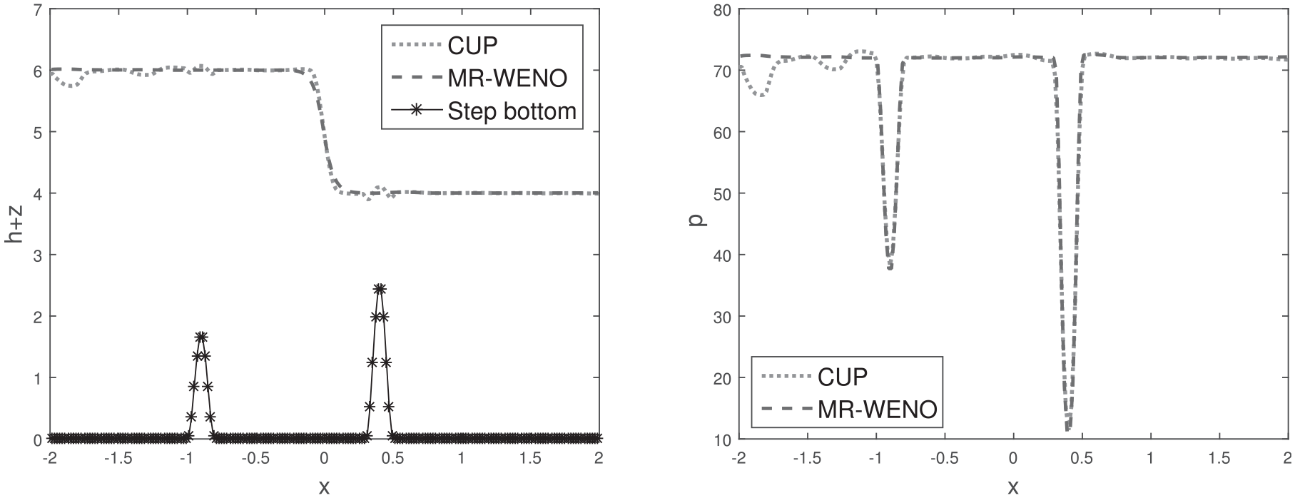
• Test problem 1: This test problem checks the efficiency of proposed numerical scheme to capture the small perturbation in steady-state solution. Consider the small perturbation $\mathrm{\Phi }(x)$ to a steady-state solution in computational domain $[-2,2]$ as

$$(h,u,\theta )(x,0)=\{\begin{array}{cc}(6-z(x)+\mathrm{\Phi }(x),0,4),\hfill & x<0,\hfill \\ \multicolumn{1}{c}{(4-z(x)+\mathrm{\Phi }(x),0,9),}& x>0,\hfill \end{array}$$

where

$$\mathrm{\Phi }(x)=\{\begin{array}{cc}0.1,\hfill & -1.5\le x\le -1.4,\hfill \\ \multicolumn{1}{c}{0.0,}& \mathrm{otherwise}.\hfill \end{array}$$

and take the following non-flat bottom topography

$$z(x)=\{\begin{array}{cc}0.85(\cos (10\pi (x+0.9))+1),\hfill & -1.\le x\le -0.8,\hfill \\ \multicolumn{1}{c}{1.25(\cos (10\pi (x-0.4))+1),}& 0.3\le x\le 0.5,\hfill \\ \multicolumn{1}{c}{0,}& \mathrm{otherwise}.\hfill \end{array}$$

The steady-state solution is a piece-wise constant steady solution. The initial surface and pressure are shown in Figure 1. Then the solutions on $200$ grid cells is obtained from FV MR-WENO and central upwind (CUP) schemes are shown in Figure 2 at time t =  $0.4$ . Clearly the numerical solutions obtained from FV MR-WENO scheme are more efficient as compare to the results obtained from CUP scheme.

• Test problem 2: This test problem taken from Snchez-Linares et al. ⁸ and is used to check the numerical order of accuracy of considered numerical algorithm for a smooth solution. Consider the domain is $[0,1]$ and simulation time t =  $1$ . The initial conditions are given as

$$\begin{array}{c}\multicolumn{1}{c}{h(x,0)=1.0-z(x),\mathrm{hu}(x,0)=0.1,\theta (x,0)}\\ =1.0+0.01\cos (2\pi (x-0.5)),\hfill \end{array}$$

and the bottom function $z(x)$ is defined as

$$z(x)=0.1\sin (4\pi x)-1.0.$$

Figure 1.

Surface and pressure at $t=0.0$ .

Figure 2.

Comparison of finite volume WENO with central upwind scheme. Surface and pressure at $t=0.4$ .

As exact solution of this problem is not known, so reference solution which computed with $4000$ cells is treated as exact solution for computing the numerical $L^1$ -errors. These errors and numerical order of accuracy for the FV MR-WENO scheme are given in Table 1, which clearly shows that fifth order accuracy is obtained.

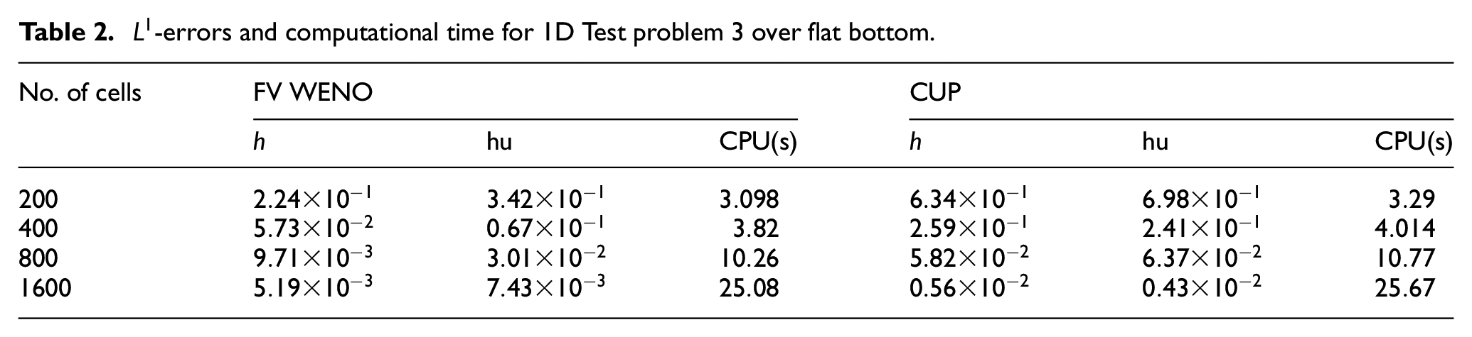
• Test problem 3: Consider the dam break problem, taken from Touma and Klingenberg, ⁹ over a flat bottom with the following initial conditions

$$(h,u,\theta )(x,0)=\{\begin{array}{cc}(5,0,3),\hfill & x\le 0,\hfill \\ \multicolumn{1}{c}{(1,0,5),}& x>0.\hfill \end{array}$$

Table 1.

$L^1$ -errors and numerical orders of accuracy for 1D Test problem $2$ .

No. of cells	h		hu		h $\theta$
	$L^1$ -error	Order	$L^1$ -error	Order	$L^1$ -error	Order
$20$	$1.17\times {10}^{-3}$	—	$2.46\times {10}^{-3}$	—	$2.26\times {10}^{-3}$	—
$40$	$3.73\times {10}^{-5}$	4.9712	$7.83\times {10}^{-5}$	4.9735	$7.07\times {10}^{-5}$	4.9985
$80$	$9.970\times {10}^{-7}$	5.2254	$2.190\times {10}^{-6}$	5.1600	$1.68\times {10}^{-6}$	5.3952
$160$	$3.10\times {10}^{-8}$	5.0073	$6.58\times {10}^{-8}$	5.0567	$5.18\times {10}^{-8}$	5.0194
$320$	$9.18\times {10}^{-10}$	5.0776	$1.98\times {10}^{-9}$	5.0545	$1.51\times {10}^{-9}$	5.1003

In Figure 3, the exact and approximate solutions on $200$ grid points are plotted in the computational domain $[-1,1]$ at time t $=0.2$ . Good agreement among analytical and numerical results verify the correctness of both numerical schemes but computation of $L^1$ -errors and computational time for both numerical schemes are mentioned in Table 2 show that the proposed numerical method is more efficient that the CUP scheme.

• Test problem 4: This test problem is taken from Touma and Klingenberg, ⁹ in which dam break problem over a flat bottom topography with initial conditions are defined as follow

$$(h,u,\theta )(x,0)=\{\begin{array}{cc}(2,0,1),\hfill & -0.5\le x\le 0.5,\hfill \\ \multicolumn{1}{c}{(1,0,1.5),}& \mathrm{otherwise}.\hfill \end{array}$$

Figure 3.

Comparison of numerical results obtained from FV MR-WENO scheme with exact Riemann solutions and solutions of CUP scheme.

Table 2.

$L^1$ -errors and computational time for 1D Test problem $3$ over flat bottom.

No. of cells	FV WENO			CUP
	h	hu	CPU(s)	h	hu	CPU(s)
$200$	$2.24\times {10}^{-1}$	$3.42\times {10}^{-1}$	$3.098$	$6.34\times {10}^{-1}$	$6.98\times {10}^{-1}$	$3.29$
$400$	$5.73\times {10}^{-2}$	$0.67\times {10}^{-1}$	$3.82$	$2.59\times {10}^{-1}$	$2.41\times {10}^{-1}$	$4.014$
$800$	$9.71\times {10}^{-3}$	$3.01\times {10}^{-2}$	$10.26$	$5.82\times {10}^{-2}$	$6.37\times {10}^{-2}$	$10.77$
$1600$	$5.19\times {10}^{-3}$	$7.43\times {10}^{-3}$	$25.08$	$0.56\times {10}^{-2}$	$0.43\times {10}^{-2}$	$25.67$

The solution profiles $h$ , $\theta$ , and $p=\frac{g{h}^2\theta }{2}$ are obtained on $200$ grid points in domain $[-1,1]$ at time t =  $0.2$ , as shown in Figure 4. Both numerical methods resolve the discontinuities in efficient way but the considered numerical method behaves more efficiently in the computation of solution profile $\theta$ .

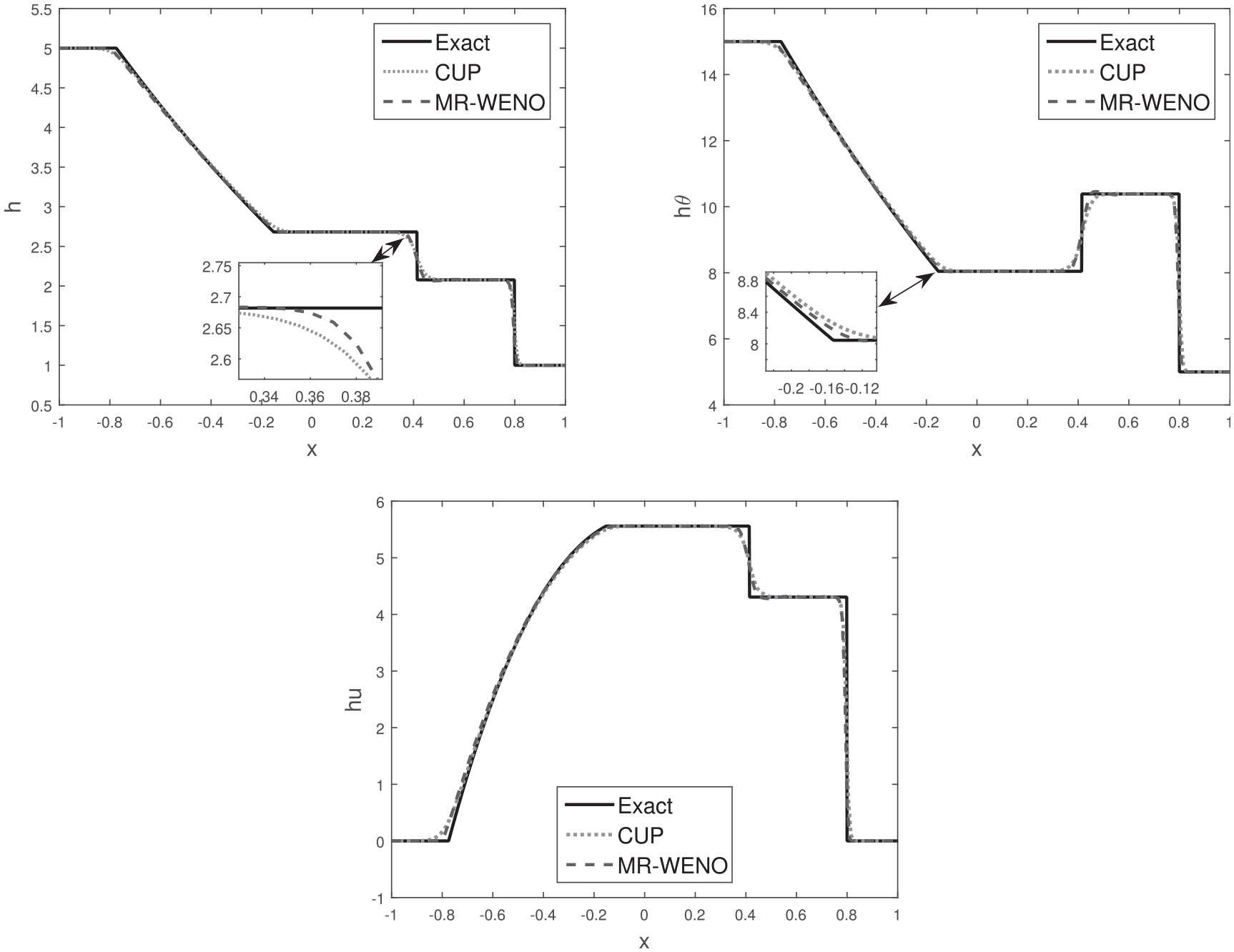
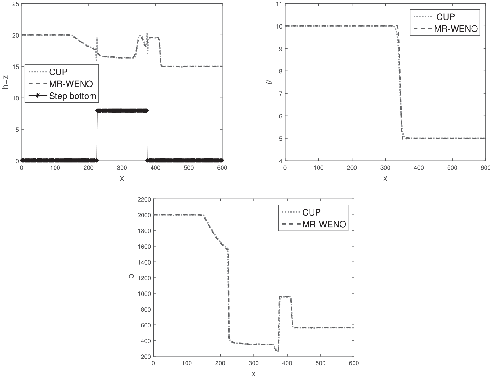
• Test problem 5: This test problem is taken from Touma and Klingenberg, ⁹ to check the efficiency of well balance FV MR-WENO scheme on non-flat bottom topography. In this test problem the step like bottom topography is considered since we have exact solution of Ripa model with step like bottom topography. The initial conditions are given by

$$(h,u,\theta )(x,0)=\{\begin{array}{cc}(25-z(x),0,10),\hfill & x\le 300,\hfill \\ \multicolumn{1}{c}{(20-z(x),0,5),}& x>300,\hfill \end{array}$$

and bottom topography is defined as

$$z(x)=\{\begin{array}{cc}8,\hfill & x>300,\hfill \\ \multicolumn{1}{c}{0,}& \mathrm{otherwise}.\hfill \end{array}$$

Figure 4.

Test problem over flat bottom topography. Comparison of numerical results obtained from FV MR-WENO scheme with CUP scheme.

The solution profiles $h$ , $\mathrm{hu}$ , and $h\theta$ on $400$ grid points in the domain $[0,600]$ at time t =  $12.0$ are shown in Figure 5. A very good agreement between exact solution and well-balanced FV MR-WENO scheme is observed in figure while central upwind scheme produces oscillation near the stationary shock wave.

• Test problem 6: Now we consider the dam break problem over a rectangular bump. ⁹ In this problem the bottom topography is defined as

$$z(x)=\{\begin{array}{cc}8,\hfill & |x-300|>275,\hfill \\ \multicolumn{1}{c}{0,}& \mathrm{otherwise}.\hfill \end{array}$$

and initial conditions are defined as

$$(h,u,\theta )(x,0)=\{\begin{array}{cc}(20-z(x),0,10),\hfill & x\le 300,\hfill \\ \multicolumn{1}{c}{(15-z(x),0,5),}& x>300.\hfill \end{array}$$

Figure 5.

Test problem for the non-flat bottom topography. Comparison of numerical results obtained from FV MR-WENO scheme with exact Riemann solutions and solutions of CUP scheme.

The computational domain $[0,600]$ is discretized into $400$ grid cells and the solution profiles $h$ , $\theta$ , and $p$ are computed at time $0.2$ , as shown in Figure 6. Once again proposed numerical scheme behaves very well over non-flat bottom topography.

Figure 6.

Rectangular dam break over non-flat bottom topography. Comparison of finite volume WENO with CUP scheme.

Two-dimensional test problems

In this subsection we present test problems for 2D Ripa model over flat and non flat bottom topographies.

• Test problem 7: Consider the two dimensional rectangular dam break problem over a flat bottom topography, taken from Touma and Klingenberg. ⁹ The initial conditions which feature two constant states are given by

$$(h,u,v,\theta )(x,y,0)=\{\begin{array}{cc}(2,0,0,1),\hfill & \mathrm{if}|x|\le 0.5,\hfill \\ \multicolumn{1}{c}{(1,0,0,1.5),}& \mathrm{otherwise}.\hfill \end{array}$$

The solution profiles $h$ , $\mathrm{hu}$ , and $h\theta$ are computed in the computational domain $[-1,1]\times [-1,1]$ at time $0.2$ using the well-balanced FV MR-WENO scheme, as shown in Figure 7. The computational domain is discretized into $100\times 100$ grid cells. Moreover the solution profiles, obtained from both numerical schemes, are drawn along $x-\mathrm{axis}$ in Figure 8. A good agreement between numerical results is observed.

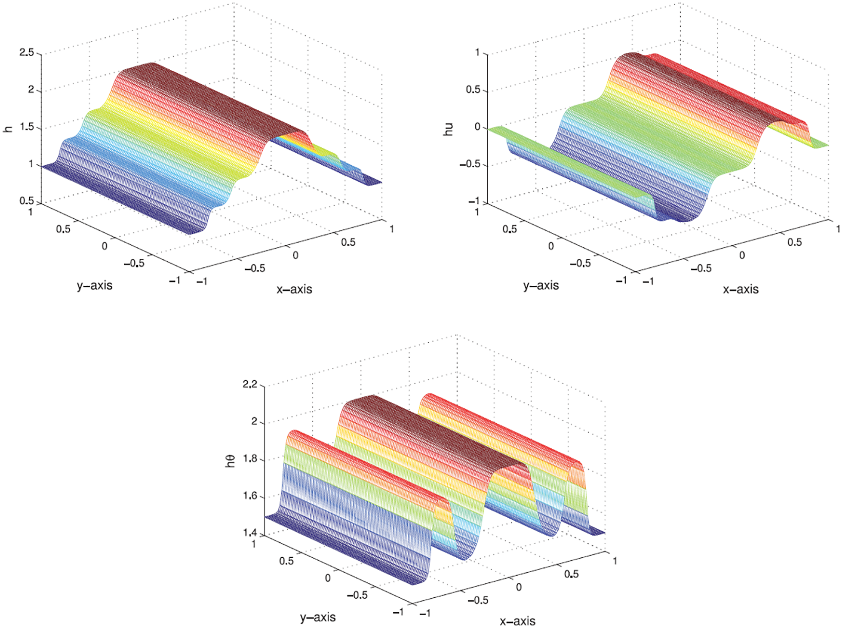
• Test problem 8: We consider the 2D steady-states problem for Ripa system. Consider the small perturbation $\mathrm{\Phi }(x,y)$ to a steady-state solution as

$$\begin{array}{c}(h,u,\theta )(x,y,0)=\hfill \\ \{\begin{array}{cc}(3-z(x,y)+\mathrm{\Phi }(x,y),0,0,4/3),\hfill & \mathrm{if}{x}^2+y^2<0.25,\hfill \\ \multicolumn{1}{c}{(2-z(x,y)+\mathrm{\Phi }(x,y),0,0,3),}& \mathrm{otherwise}.\hfill \end{array}\hfill \end{array}$$

where

$$\mathrm{\Phi }(x)=\{\begin{array}{cc}0.1,\hfill & \mathrm{if}0.01\le x^2+y^2<0.09,\hfill \\ \multicolumn{1}{c}{0.0,}& \mathrm{otherwise}.\hfill \end{array}$$

and take the following non-flat bottom topography

$$\begin{array}{c}z(x,y)=\hfill \\ \{\begin{array}{c}0.5\exp (-100((x+0.5{)}^2+(y+0.5{)}^2)),\mathrm{if}x\le 0,\hfill \\ \multicolumn{1}{c}{0.6\exp (-100((x-0.5{)}^2+(y-0.5{)}^2)),\mathrm{otherwise}}\end{array}.\hfill \end{array}$$

Figure 7.

Rectangular dam break over flat bottom.The solution profiles are computed by well-balanced finite volume WENO scheme.

Figure 8.

Rectangular dam break over flat bottom.Comparison of finite volume WENO scheme with central upwind scheme.

The solution profiles $h+z$ , $u$ , and $\theta$ are computed in the computational domain $[-1,1]\times [-1,1]$ at time $0.2$ using the well-balanced FV MR-WENO scheme, as shown in Figure 9. The computational domain is discretized into $200\times 200$ grid cells. Moreover the solution profiles, obtained from both numerical schemes, are drawn along $x$ - $\mathrm{axis}$ in Figure 10. Clearly from Figure 10, the results of proposed numerical scheme are far better as compare to central upwind scheme.

• Test problem 9: This test problem ³³ is used to check the numerical order of accuracy of proposed numerical scheme for a smooth solution. Consider the computational domain is $[0,1]\times [0,1]$ and simulation time $t=0.035$ . The initial conditions are given by

$$\begin{array}{c}h(x,y,0)=10.0+\exp (2\pi x)\cos (2\pi y),\hfill \\ \mathrm{hu}(x,y,0)=\sin (\cos (2\pi x))\sin (2\pi y),\hfill \end{array}$$

$$\begin{array}{c}\mathrm{hv}(x,y,0)=\cos (\sin (2\pi y))\cos (2\pi x),\hfill \\ \theta (x,y,0)=\cos (x)\sin (y),\hfill \end{array}$$

and the bottom function $z(x)$ is defined as

$$z(x,y)=\sin (2\pi x)+\cos (2\pi y).$$

Figure 9.

Small perturbation of steady-state.

Figure 10.

Comparison of finite volume WENO scheme with central upwind scheme.

As exact solution of this problem is not known, so reference solution which computed on $1000\times 1000$ grid cells is treated as exact solution for computing the numerical $L^1$ -errors. These errors and numerical order of accuracy for the FV MR-WENO scheme are given in Table 3, which clearly shows that fifth order accuracy is obtained in 2D case.

Table 3.

$L^1$ -errors and numerical orders of accuracy for 2D Test problem $9$ .

No. of cells	h		hu		hv		h $\theta$
	$L^1$ -error	Order	$L^1$ -error	Order	$L^1$ -error	Order	$L^1$ -error	Order
$20\times 20$	$2.11\times {10}^{-3}$	—	$2.01\times {10}^{-3}$	—	$2.01\times {10}^{-3}$	—	$1.11\times {10}^{-3}$	—
$40\times 40$	$8.33\times {10}^{-5}$	4.66	$7.81\times {10}^{-5}$	4.68	$7.71\times {10}^{-5}$	4.70	$3.63\times {10}^{-5}$	4.9344
$80\times 80$	$2.59\times {10}^{-6}$	5.00	$2.49\times {10}^{-6}$	4.97	$2.39\times {10}^{-6}$	5.01	$9.19\times {10}^{-7}$	5.3038
$160\times 160$	$7.98\times {10}^{-8}$	5.02	$7.50\times {10}^{-8}$	5.05	$7.44\times {10}^{-8}$	5.00	$2.58\times {10}^{-8}$	5.1546
$320\times 320$	$2.49\times {10}^{-9}$	5.01	$2.31\times {10}^{-9}$	5.02	$2.30\times {10}^{-9}$	5.01	$7.81\times {10}^{-10}$	5.0459

Conclusions

Well-balanced FV MR-WENO schemes were derived to solve the 1D and 2D Ripa models. Despite the presence of temperature gradients and source terms in the considered models, the derived numerical schemes exactly held the steady-state solutions, maintained the high order accuracy for smooth solutions, and suppressed the unwanted oscillations near the strong shock transitions. Different 1D and 2D numerical test problems were computed to check the validity of designed numerical algorithms qualitatively and quantitatively. The numerical results of derived numerical algorithms were compared with those obtained from the exact solutions and CUP schemes. A very good agreement was seen among the results of designed numerical schemes and exact Riemann solver for the Ripa system. However, the proposed schemes have produced better results as compared to the CUP schemes.