
Abstract
Identification of optimal features is necessary for the decision-making models such as the artificial neural network to achieve effective and robust on-line monitoring of cutting tool condition. Most feature selection strategies proposed in the literature are for pattern recognition or classification problems, and not suitable for prognostic problems. This paper applies three parameter suitability metrics introduced in previous similar studies for failure-time analysis and modifies them for failure-process analysis which allows for the unit-wise variation of the component in a population. The suitability of a feature used for cutting tool condition monitoring is determined by its fitness value calculated based on the three metrics. Two types of recurrent neural network are employed to analyze the prognostics ability of the features extracted from multi-sensor signals (acoustics emission, motor current, and vibration) collected from a milling machine under various operating conditions. The analysis results validate that the fitness value of a feature can depict its prognostic ability. It is found that adding more features which share abundant information does not increase the prediction performance but increases the burden on the decision-marking models. In addition, adding features with low fitness values may even deteriorate the prediction.
Introduction
On-line cutting tool wear monitoring plays a critical role in industry automation and has the potential to significantly increase productivity and improve product quality. In the literature, a significant amount of research work has been performed dealing with machine tool condition monitoring (TCM).1–3 A variety of sensors can be employed to capture tool wear condition. Acoustic emission (AE), force, vibration, temperature and motor current sensors are the most commonly used sensors reported in the literature.4,5 However, different types of signals may respond differently to the tool condition during different machining applications (milling, turning, grinding, etc.). 6 Thus, the so-called sensor fusion is becoming a prevailing concept in the sensor-based tool condition monitoring.
Although sensor signals contain sufficient tool condition information throughout a machining process, they are convoluted with noise from the cutting operation. Therefore, feature extraction becomes necessary in order to maximize the information utilization of sensor signals. A variety of typical monitoring indices can be obtained from the time-domain and frequency-domain features. 7 Advanced signal processing techniques such as mel-frequency cepstral coefficient 8 and S-transform 9 have also been employed by some researchers to extract features that represent the characteristics of the cutting process (information) and to separate these features from various noise disturbances. However, features extracted from an independent data source are not equally informative: certain features may correspond to noise, not information; others may be correlated or not relevant to the target. Therefore, the successful selection of effective features describing the characteristics of the cutting process is a significant task for an accurate and robust on-line system for monitoring of tool conditions.
Compared with other commonly used data-driven prognostic methods, such as the support vector machine, 10 Bayersian approaches, 11 neuro-fuzzy techniques 12 and stochastic degradation model, 2 the artificial neural networks (ANNs)13,14 are the most popular data-driven models that are widely used as the decision-making systems for the cutting tool condition monitoring. The feasibility of using neural networks to integrate information from multiple sensors to monitor tool conditions in machining has been demonstrated by many studies in the literature. Optimization algorithms such as the genetic algorithm and the particle swarm optimization algorithm were used to optimize the neural network model for better predictions of the grinding parameters in some works.15,16 Since 2006, deep learning has become a rapidly growing research, and is adopted by many researchers as a bridge connecting multi-sensor time-series data and intelligent machine health monitoring. 17 For instance, Aghazadeh et al. 3 employed the convolutional neural network as a well-established deep learning algorithm for tool wear estimation. Yu et al.18,19 proposed a bidirectional recurrent neural network (BiRNN) based encoder-decoder scheme to obtain an unsupervised health index from the multi-sensor time-series data collected from a milling machine, based on which the degradation path of the cutting tool was established. Recently, Agarwal and Desai 20 proposed a hybrid model that integrates the merits of a physics-based model and a data-driven model for the estimation of cutting forces during the end milling operation. The physics-based model establishes an explicit relationship between the process variables and attributes based on scientific knowledge whereas the data-driven model was used to learn their relationship which can be easily scaled to accommodate new variables and attributes without conducting numerous experiments.
It is well accepted that the prediction performance of a decision-making system is closely related to the features fed into it. Thus, identification of optimal features for an effective and robust on-line monitoring of tool wear is necessary.
The literature reports abundant feature selection strategies including partial least squares (PLS) method, 21 euclidean distance evaluation technique, 7 principle component analysis, 22 and dominant feature identification. 23 Basically, the key idea behind these methods is to find a mapping from the original higher dimensional feature space to a lower dimensional feature space. However, these methods are mainly for pattern recognition and general classification problems. For prognostic problems, the above methods become inapplicable as the features extracted inherently are not obtained under a fixed pattern or condition. Traditionally, identification of the optimal prognostic features (or monitoring parameters) is accomplished through visual inspection of the available information and engineering judgment. 24 However, it is usually time-consuming and ineffective. Automated selection of the optimal features is therefore required. Some researchers have proposed several metrics to characterize the suitability of a feature used for prognostic problems. Scheffer and Heyns 25 introduced two methods to select the most reliable features that correlate best with the cutting tool condition, which are based on the correlation between the feature and the objective, and the statistical overlap factor (SOF). Javed et al. 26 proposed the cumulative features that have high monotonicity and trendability with the degradation process of the component, which were proved to surely enhance prognostics modeling. Guo et al. 27 used the monotonicity and correlation metrics to select the most sensitive features, which were subsequently fed into a recurrent neural network (RNN) for the RUL prediction of bearings. Coble and Hines 24 introduced three parameter suitability metrics to identify an ideal prognostic feature: monotonicity, prognosability, and trendability. A big step forward in this research is that the feature selection strategies were moved from failure-time analysis to failure-process analysis, which allows for the unit-wise variations in a population.
From the above literature review, most of the widely used feature selection strategies were aimed at pattern recognition and classification problems such as machine fault detection or diagnosis. For prognostic problems such as continually monitoring the degradation process of a system, or the prediction of remaining useful life (RUL) of a component, these strategies become inapplicable as the features extracted inherently are not obtained under a fixed pattern or condition. Although there were a few attempts in assessing the suitability of the monitoring features for prognostics of a component, different researchers preferred different parameter suitability metrics for different monitoring applications. Plus, most of the suitability metrics correspond to the failure-time analysis, which uses the failure times recorded during normal operation to estimate the RUL for a population of identical components. However, it is more often that individuals from a population of identical components deviates slightly in the normal degradation path over time due to unit-wise variations.24,28 Thus, parameter suitability metrics based on the failure-process analysis using degradation measures are more practical and reliable to assess the prognostic ability of a feature.
This study proposed a method to directly calculate the fitness of a feature which assesses the prognostic ability of the feature based on three suitability metrics. The proposed method allows for the effect of unit-wise variations of the monitoring system because the three metrics are calculated based on degradation measures (e.g. tool wear, crack size) instead of degradation time. Two types of recurrent neural network are employed to analyze the prognostics ability of the features extracted from multi-sensor signals (acoustics emission, motor current, and vibration) collected from a milling machine under various operating conditions. The analysis results validate that the fitness value of a feature can depict its prognostic ability.
This paper is organized as follows: Section 1 reviews previous similar studies regarding the sensor-based tool condition monitoring system. Limitations of previous feature selection methods are pointed out, from which the objective of the current research is stressed. Section 2 presents three modified parameter suitability metrics based on the failure-process analysis, from which the fitness of a feature can be determined. The two types of recurrent neural network, which are used as the decision-making models to predict the tool wear in this study are also illustrated in this section. Section 3 first describes an experimental milling data set, based on which the fitness values of 10 features extracted from five sensors (AE, vibration, and current) are determined. After that, the RNNs are employed to predict tool wear based on the selected features. The prediction error distribution of each feature set is expressed by using the boxplot in order to holistically compare the prediction performance among different feature sets fed into the RNNs. The main conclusions of this study are provided in the last section.
Methodology
Fitness of a feature
Identification of appropriate prognostic features that are provided as inputs to decision-making models is key for reliable on-line condition monitoring of tool wear. There are several criteria that can be used to select the most reliable features which correlate best with tool condition.
Correlation coefficient COR
When using the failure-time analysis (usually for long-term degradation of a component such as bearings), the operating time of the individual component is used as the degradation measure. The linear correlation between the feature q and operating time t is calculated by 27 :

where qi, ti are the values of the feature and the corresponding operating time of the ith observed sample, respectively.
When using the degradation measure (usually for short-term degradation such as cutting tool wear), the amount of tool flank wear (VB) in the cutting tool condition monitoring application, the correlation between the feature q and the objective VB (the amount of tool wear) can be calculated according to:

where VBi is the amount of tool wear of the ith observation sample.
Monotonicity coefficient MON
The monotonicity characterizes the underlying increasing or decreasing trend of a time series with the gradual increase of the time values. This metric has been used to select the features indicating gradual degradation (usually long-term) of mechanical components, such as bearings and gears, as it is generally assumed that the monitoring components do not undergo self-healing.24,26,27 When using the failure-time analysis, the monotonicity metric evaluates the increasing or decreasing trend of the feature q with the operating time as expressed by:
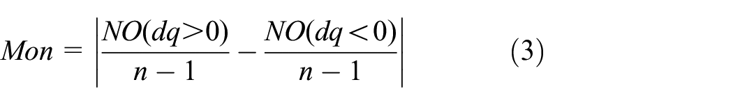
where dq is the differential of feature series q; NO (dq > 0) and NO (dq < 0) represent the numbers of dq that are positive and negative, respectively.
When using the degradation measure, the monotonicity between the feature q and the objective VB (the amount of tool wear) can be calculated as:

where dVB is the differential of the objective VB. The monotonicity between the feature q and the objective VB indicates the consistency of the variations of the feature (increasing or decreasing) with the variations of the objective. The higher the value of MON, the more consistency of the variations of the feature with the variations of the objective.
Statistical overlap factor SOF
The statistical overlap factor (SOF) is a metric which can determine the degrees of separation of a feature q under different operating conditions, 25 for instance, the cutting speed S, depth of cut D, and feed F in the cutting tool condition monitoring application. Ideally, a good feature should show a high degree of separation under different operating conditions, and a low degree of separation due to noise. The SOF of a feature q obtained from two different operating conditions (condition i and condition j) can be calculated as:
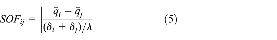
where

The SOF of a feature q calculated by equation (6) indicates its ability to distinguish among different operating conditions. A higher value of SOF represents that the feature shows a stronger variation due to the change of operating conditions rather than the noise.
Fitness FIT
The suitableness of a feature used for cutting tool condition monitoring can be defined as a weighted sum of the above three mentioned metrics24,27:

where a, b, c are the weights of the correlation coefficient COR, the monotonicity coefficient MON and the statistical overlap factor SOF, respectively. In addition, the sum of their values should be 1. Obviously, the values of these weights determine the contributions of the three metrics on the final feature selection criteria FIT. The exact weight coefficients for the three metrics are hard to theoretically determined. A good monitoring feature should not only have good correlation and monotonicity with the degradation measure, but also a stronger variation due to the change of operating conditions rather than noise. Assigning same weight coefficients to them seems a reasonable idea. 27 However, unequal weights can also be assigned if a metric needs more consideration depending on the specific application. 24
Decision-making models
In this study, in order to demonstrate that the proposed methodology is not model-specific, we used two types of recurrent neural network as the decision-making models to predict the tool wear: Elman network and long short-term memory (LSTM). Compared with feedforward neural networks, RNNs have loops in them, which allows information to be passed from a previous time step of the unit to the next as shown in Figure 1. Therefore, unlike feedforward neural networks (FFNN), RNNs possess an internal memory that can make use of past information, which makes it especially suitable for processing sequential data or time series data. In fact, the FFNNs are normally used for pattern recognition or classification problems especially when the input data do not possess explicit time dependencies, whereas the RNNs are more powerful in dealing regression modeling or prognostic problems as the degradation of a mechanical component is usually a time-dependent, continuous, monotonical phenomenon.20,29

The recurrent neural network.
An Elman network is typically a three-layer network (input, hidden, and output). The outputs from the hidden layer in the previous time step are also fed into the input layer in the current time step. It is usually trained using classic backpropagation through time. 27 However, traditional RNNs are only capable of handling time series (sequences) with short-term dependencies (short time span between the point with the relevant information and the point to be predicted) due to the problem of gradient vanishing and/or exploding during training. The long short-term memory was first introduced by Hochreiter and Schmidhuber 30 to overcome the vanishing gradient problem. It has a similar chain-like structure as shown in Figure 1. However, instead of having a simple unit inside the hidden neurons, the LSTMs have three gates (input gate, forget gate, and output gate) and one cell interacting inside each of their hidden neurons, as shown in Figure 2. These gates are used to control the passing of information along the sequences, which can be mathematically expressed as.18,27,31,32
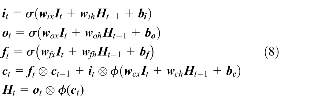
where

The architecture of a hidden neuron for: (a) Elman network and (b) LSTM.
Discussions and results
Milling data set
The experiment was done on a milling machine which describes the tool wear process under various operating conditions. 33 The workpiece material is cast iron. The cutting speed was constant at 200 m/min (826 rev/min). Two different depths of cut (1.5 mm and 0.75 mm), and two feed rates (0.5 mm/rev and 0.25 mm/rev) were investigated. The experimental matrix is 2 × 2. Hence there are four different cutting conditions, as shown in Table 1. The experiment under each condition was done a second time with a second set of inserts. Therefore, there are eight cases with a variable number of runs per tool life. The number of runs was dependent on the degree of flank wear that was measured between runs at irregular intervals up to a set wear limit. There is a total of 108 data samples.
Milling data set.

Three types of sensor (two AE sensors, two accelerometers and a current sensor) were adopted to acquire the AE signals, the vibration signals at different positions, and the AC spindle motor current. Since the data were collected from a real milling machine (instead of simulation models or experimental platforms) working under operational conditions close to industrial applications, it provides important information for researchers to study the relationship between health states and measurements.9,34,35 In addition, we propose to use the leave-one-out cross-validation method to cope with the overfitting problem caused by the limitation regarding the number of samples. By doing so, we deem the milling data set is sufficient for an effective study as conducted in this paper. In this study, we select 10 common features used in cutting tool condition monitoring as listed in Table 2, which includes four time-domain dimensional statistical features (peak to peak, root mean square, standard deviation, peak), two time-domain dimensionless features (kurtosis, crest factor), two frequency-domain features (amplitude of the first harmonic, average of the first six harmonic amplitudes), and two statistical features based on the β-distribution (skewness and kurtosis based on the β-distribution). The first eight are classic features used in the condition monitoring of mechanical system, whereas the last two were introduced by Kannatey-Asibu and Dornfeld 36 to monitor the tool wear.
Features used in this study.

Based on equations (2), (4), and (6), the three metric values of the ten selected features (as shown in Table 2) from the five sensors are shown in Figure 3. The final fitness for each feature from each sensor is calculated based on equation (7) by using the same weight coefficient for the three metrics, and listed in Table 3. It can be observed that the features from the motor current have generally higher fitness values than the features from the other sensors, followed by the features of the table AE. The spindle vibration provides the features with the lowest fitness values. This indicates that the features from the motor current and the table AE may provide better prognostic ability for the tool flank wear, whereas the features from spindle vibration offer the poorest prognostic ability. This phenomenon is consistent with the findings concluded from previous similar research activities: AE signals and cutting forces generally offer much richer information18,36,37; the less costly and easily mountable motor current sensor can be a fairly good substitute of the dynamometer (force sensor) as the spindle motor current is well correlated with the cutting force. 6 Besides, it can also be found that, generally, the four time-domain dimensional features (1, 2, 3, 4 in Table 2) show higher fitness values, followed by the two β-distribution moments (9, 10 in Table 2), and the two frequency-domain features (7, 8 in Table 2). The two time-domain dimensionless features (5, 6 in Table 2) have the lowest fitness values for most sensors.
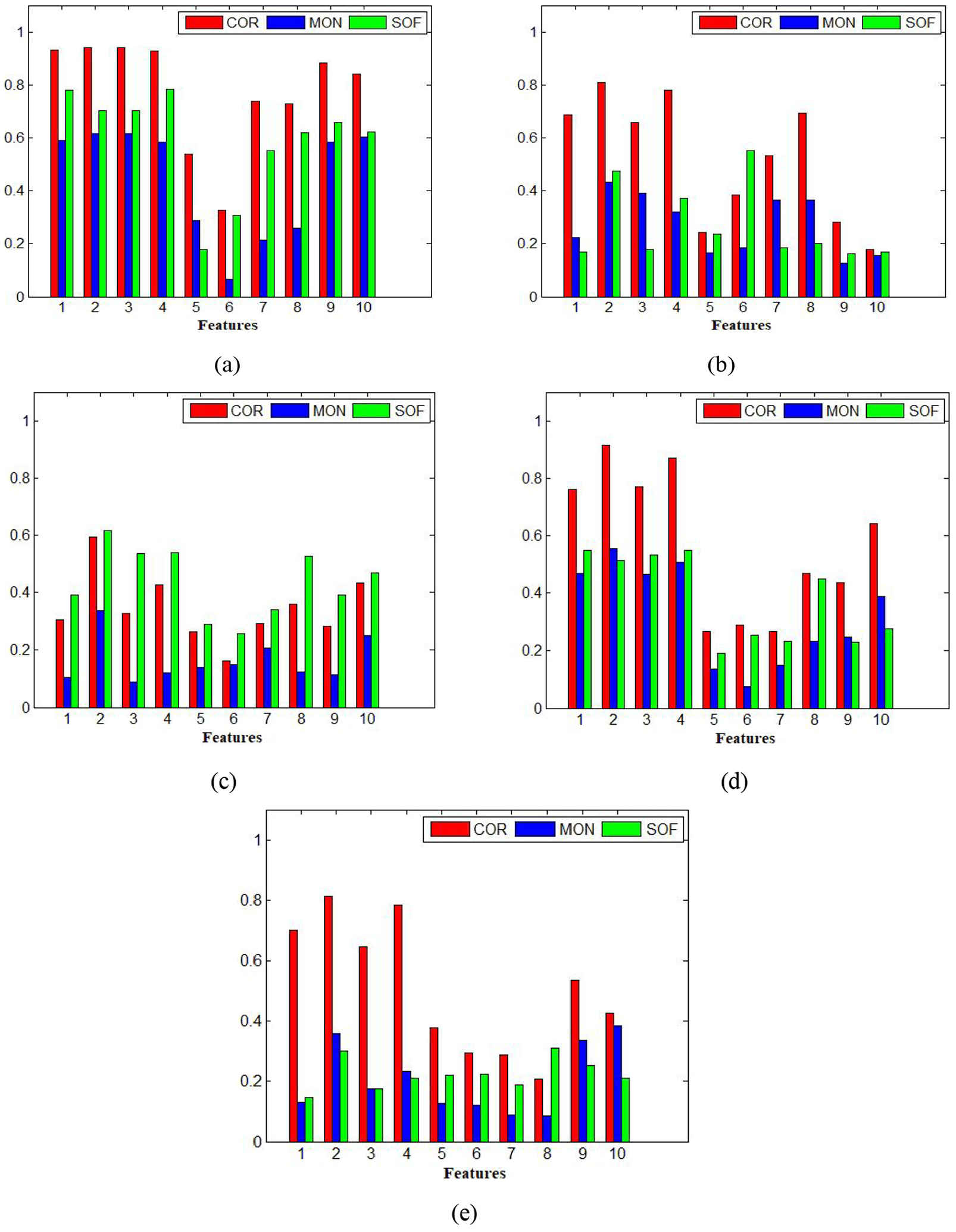
Values of the three metrics for the ten selected features from different sensors: (a) motor current, (b) table vibration, (c) spindle vibration, (d) table AE, and (e) spindle AE.
Fitness of the ten features of the five sensors.

Predictions based on the RNNs
All 108 samples from the milling data set are arranged sequentially 38 and shown in Figure 4: the first tool set operates under the four cutting conditions sequentially, and then the second tool set undergoes the same order. Since the samples are limited, we use the leave-one-out cross-validation method to train the network in order to remedy issues like overfitting and selection bias, as suggested by Malhotra et al. 39 This is done by defining a moving window with a given width which is about ¼ of the total samples (i.e. 27 samples) as the validation set, whereas the rest 81 samples as the training set for model training to predict those 27 validation points. To cover all possible combinations, the window is slid along the entire data (as shown in Figure 4) so there are 108 times of training and validation. The average of the validation errors is used to assess the prognostic abilities of different input sets. This strategy ensures the decision-making models we developed generalize well on the milling datasets. We further run the leave-one-out cross-validation 10 times for each input set to cope with the stochastic process caused by the randomly set initial parameters of the neural networks. Comparisons among the error distributions yielded by neural networks fed with different inputs can provide us a holistic impression on the prognostic ability of each input feature set.

Sliding window on the sequence of the tool wear.
As to the network parameters, their values should be kept same for different input sets so that the comparisons are effective. The learning rate for training LSTM should be much smaller than that for training Elman network to avoid the gradient exploding possibly due to its much more complex architecture (note that the LSTM can only handle the gradient vanishing problem). The details of the RNN parameters chosen for comparisons are summarized in Table 4.
Details of the RNNs.

Prediction accuracy of each feature from each sensor
In this section, we will compare the prediction errors (which is defined as the root mean square error between the predicted values and actual values of the wear for the validation set as shown in Figure 4) among the networks fed with different feature vectors, in order to find out if the fitness value of a feature truly reflects its prognostic performance. The feature vector

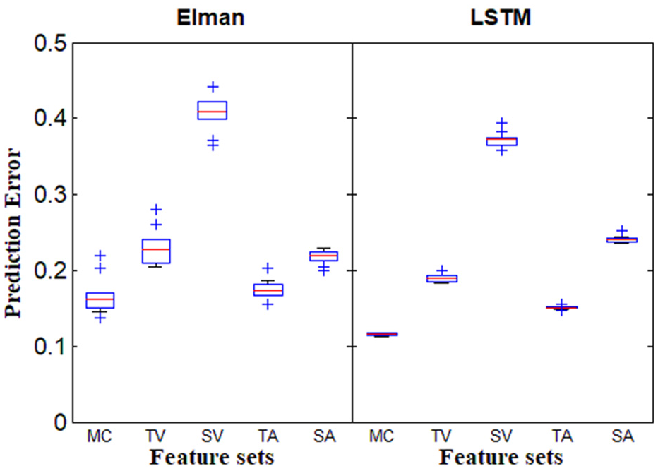
Figure 5 shows the boxplots of the prediction errors for all cases (10 features × 5 sensors × 2 RNNs). It can be noticed that the features with higher fitness values shown in Table 3 generally yield smaller prediction errors from both the Elman network and LSTM network. For instance, the first four features for each sensor generally yield lower prediction errors compared with others. The last two features of the motor current (Figure 5(a)) also yield comparatively lower prediction errors. The features of the spindle vibration (Figure 5(c)) yield poorest prediction performance. All these phenomena are largely consistent with the fitness values shown in Table 3. Thus the fitness value calculated from equations (1) to (7) truly reflects the prognostic ability of a feature. On the other hand, comparisons between the prediction errors from the Elman network and LSTM network show that the LSTM slightly outperforms the Elman network in yielding smaller and more stable prediction errors in most cases. However, the training time for the LSTM is considerably longer than that of the Elman network (considering that LSTM has 4 units in each of its hidden neurons to be trained in comparison to the one unit of that of Elman).

Boxplots of the prediction errors from each feature of each sensor: (a) motor current, (b) table vibration, (c) spindle vibration, (d) table AE, and (e) spindle AE.
Prediction accuracy of each sensor
In the section, we will investigate which sensor signal contains sufficient information of the tool condition. This is conducted by setting the feature vector

where S1 … S10 represent the 10 features of a sensor signal (
Figure 6 shows the boxplots of the prediction errors based on the 10 features extracted from each sensor. The spindle vibration still performs the worst, followed by the table vibration. This indicates that the vibration signals are truly less sensitive to the cutting tool condition compared with the motor current signal and acoustic emission signals. The features extracted from the motor current yield the lowest prediction error among all the features, which is reasonable as the fitness values of the features extracted from the motor current are generally higher than those from other sensors. The features extracted from the acoustic emission at the table (TA) also show good prediction accuracy. However, the features extracted from the acoustic emission at the spindle seems to have less correlation with the tool condition compared with the abovementioned two sensors. Thus, it can be concluded that the motor current signal and the acoustic emission at the table contain more information regarding the tool condition. These two signal sources should be the focus for effective and reliable on-line monitoring of tool wear. It should be further noted that all these phenomena are nearly consistent with the fitness values shown in Table 2.
Boxplots of the prediction errors based on the 10 features extracted from each sensor.
Prediction accuracies of some fusing features
It is traditionally believed that an increase in the number of sensor features generally improves the performance. In this section, we investigate the prediction errors from different feature sets extracted from the motor current and the table AE as shown in Figure 7. The labels in the horizontal axis of Figure 7 represent different feature sets as illustrated in Table 5. For example, MC17 means that the feature vector has four inputs: peak to peak of the motor current signal, first harmonic amplitude of the motor current, depth of cut, and feed rate.

Boxplot of the prediction errors based on different feature sets extracted from the motor current and the acoustic emission at table.
Feature vectors I corresponding to the horizontal labels in Figure 7.

Refer to Table 3 for the symbols in I.
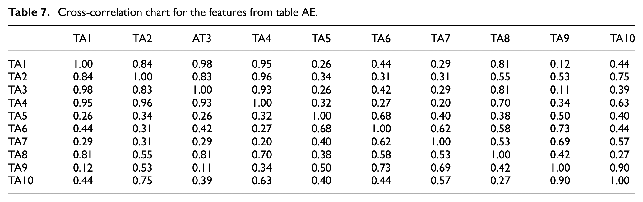
It can be found from Figure 7 that for the motor current signal, the parameter P2P (MC1) alone can achieve slightly better prediction accuracy with that achieved by combining P2P and PKS1 (MC17), or even all 10 features (MC1-10). This indicates that adding more features from the motor current signal into the feature vector does not yield a more accurate prediction. In fact, adding features with lower fitness values may even deteriorate the predictions, as also confirmed by Rangwala and Dornfeld. 40 Table 6 shows the cross-correlation chart of features from the motor current. It can be found that there are high correlations between the P2P with most of the other features from the motor current, which indicates that these highly correlated features contain abundant information with cutting process. This probably explains why only one typical time-domain statistical feature (normally RMS) of the cutting force signal or motor current signal is normally employed as the input of decision-making models in many previous similar studies.6,22,41 For the table AE signal, the combined feature set of P2P and PKS1 can achieve much better results than each alone does. This demonstrates that adding features with high fitness values but low correlations among each other can generally improve the prediction performance.
Cross-correlation chart for the features from motor current.

Tables 6 and 7 show the cross-correlation charts for the features from the motor current and table AE, respectively. It can be found that there are high correlations among most of the selected features from the motor current. This demonstrates that the selected features from the motor current have abundant information relating to the cutting process. On the other hand, the features from the table AE have comparatively lower correlations among each other, which means that these features may provide corroborative information.
Cross-correlation chart for the features from table AE.
It can be concluded that an optimal feature set should contain features that have higher fitness values, as well as lower correlations with other features. Based on the fitness values and the cross-correlation values, the following features are selected as the inputs to the networks:

Figure 8 shows the comparisons of the prediction errors based on four feature sets. The first feature set MC1-10 is all the 10 features of the motor current. The second feature set TA1-10 is all the 10 features of the table AE. The third feature set MC1-10_TA1-10 is all the 20 features from the motor current and the table AE. The forth feature set is the optimal feature set which has only three features from the sensors as shown in equation (11). Table 8 shows the prediction performance in terms of the average training time and average prediction error after 10,000 training epochs. It can be found that fusing the motor current and table AE can generally improve the prediction performance. However, some features may provide abundant information, and some others may deteriorate the predictions. After deleting these features, the optimal feature set outperforms all the others. Since there are only 71 training samples available, the training time of the optimal feature set is only slightly smaller than those of the others. The training time saved by using the optimal feature set will be much more significant if hundreds or thousands of samples are trained. It can also be found that the LSTM network yields more accurate tool wear predictions (lower prediction error) than the Elman network does on the studied milling data set. This is due to the gating mechanism (input gate, forget gate, and output gate) introduced in the hidden neurons for LSTM as shown in Figure 2. This gating mechanism enables the LSTM to adaptively control the information passing through the hidden neurons (as to what to input, what to forget and what to output). However, since the LSTM has three more gates to be trained, the training time for LSTM is much longer than the Elman network. As shown in Table 8, the training time for LSTM is generally twice as longer as that for Elman network. Considering that the networks are usually trained off-line, the expensive computation caused by training LSTM doesn’t pose a significant problem. In conclusion, the LSTM network is better than the Elman network in predicting the milling tool wear.

Boxplot of the prediction errors based on different feature sets extracted from the motor current and the acoustic emission at the table.
Comparisons in prediction performance among four feature sets.

Conclusion
Identification of the optimal features from a variety of sensors is necessary for reliable and effective on-line monitoring of cutting tool condition. This study introduces parameter fitness to determine the prognostic ability of a feature. It is calculated based on three modified parameter suitability metrics, which allows for the unit-wise variation of the component in a population. The publicly available milling data set provided in the literature are analyzed, from which ten common features from five sensors are extracted. Two types of recurrent neural network (Elman and LSTM) are employed as the decision-making models to predict the tool wear based on the selected features. The leave-one-out cross-validation method is adopted to cope with the limited number of training samples. Due to the usual random initialization of the neural networks’ parameters (weights and biases), the neural network prediction for each setting is done 10 times. The prediction error distribution for each feature set fed into the neural networks is expressed by the boxplot, so that a holistic comparison of prediction performance among different feature sets can be conducted. The main conclusions of this study include:
Three metrics (correlation, monotonicity, and the statistical overlap factor) can be used to determine the general fitness of a feature used for prognostics. A feature having a higher fitness value is proved to yield a smaller prediction error.
Features that have high correlation among each other may provide abundant information relating to the cutting tool condition. Adding more correlated features will not increase the prediction accuracy, but will increase the burden on the decision-making models. In addition, adding features that have lower fitness values may deteriorate the prediction performance. Generally, a feature that has a higher fitness, and lower correlations with others is preferred.
Different types of signal sources (motor current and table AE in this case) may provide corroborative information for tool condition monitoring. Thus, fusing features from different sensors can generally improve the prediction performance. The optimal feature set after deleting those unnecessary features can outperform the other feature sets in terms of prediction accuracy and training time.
It should be mentioned that the above three conclusions regarding the determination of optimal features for condition monitoring are adequately generic for sensor-based prediction of gradual damage in mechanical systems.
Footnotes
Handling Editor: James Baldwin
Declaration of conflicting interests
The author(s) declared no potential conflicts of interest with respect to the research, authorship, and/or publication of this article.
Funding
The author(s) disclosed receipt of the following financial support for the research, authorship, and/or publication of this article: The authors acknowledge support provided by the Natural Sciences and Engineering Research Council of Canada (Grant number: RGPIN/05922-2014).