Fault diagnosis method of rolling bearings Based on SPA-FE-IFSVM

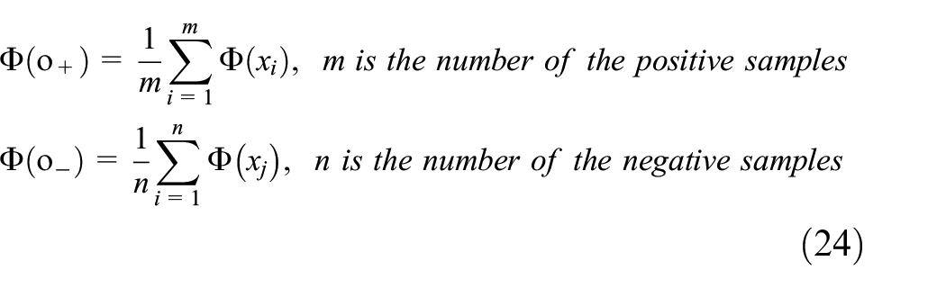
Abstract

Rolling bearings are the most frequently failed components in rotating machinery. Once a failure occurs, the entire system will be shut down or even cause catastrophic consequences. Therefore, a fault detection of rolling bearings is of great significance. Due to the complexity of the mechanical system, the randomness of the vibration signal appears on different scales. Based on the multi-scale fuzzy entropy (FE) analysis of the vibration signal, a rolling bearing fault diagnosis method based on smoothness priors approach (SPA) -FE-IFSVM is proposed. The SPA method was used to adaptively decompose the vibration signal and obtain the trend item and de-trend item of the vibration signal. Then the fuzzy entropy of the trend item and de-trend item was calculated respectively. Meanwhile, aiming at the problem that the support vector machine (SVM) cannot process the data set containing fuzzy messages and was sensitive to noise, the fuzzy support vector machine (FSVM) was introduced and improved, and then the FE as the feature vector was input into the improved fuzzy support vector machine (IFSVM) to identify the failure. The method was applied to the rolling bearing experimental data. The analysis results show that: this method can achieve 100% fault diagnosis accuracy when only two component features are extracted, which can effectively realize the fault diagnosis of rolling bearings.

Introduction

Rolling bearing is one of the most basic parts in mechanical equipment, known as “Industrial Joint,” and have the most extensive application in aerospace, electric power, metallurgy and other industries. Since the working environment of rolling bearings is usually under severe working conditions such as alternating load, high temperature and heavy load, the operating conditions of rolling bearings directly affect the working performance and service life of the entire equipment to a certain extent. ¹

When there is the local damage to the bearing, it will cause the abnormal vibration of the mechanical equipment, which is more likely to lead to the damage of the equipment. ² Therefore, it is very important to realize accurate fault diagnosis of rolling bearing. In the working process, the rolling bearing is affected by nonlinear factors such as load, friction, impact, and complex working environment, and its vibration signal presents strong nonlinear and non-stationary characteristics. ³ Therefore, the first task to realize the fault diagnosis of rolling bearings is to perform nonlinear analysis on the vibration signals of the rolling bearing and extract the fault features from the nonlinear and non-stationary vibration signals. Based on chaos theory, Lyapunov index was used to analyze the rotation frequency of the bearing in the literature. ⁴ In the literature, ⁵ the correlation dimension was introduced to realize aeroengine state monitoring and fault identification. In the literature, ⁶ the generalized fractal dimension was proposed to realize engine fault diagnosis. In these nonlinear theories, both correlation dimension and generalized fractal dimension have problems of insufficient data length and accuracy. Lyapunov index is susceptible to noise interference in the use process, which limits its practical application. In these nonlinear theories, the correlation dimension and the generalized fractal dimension all have problems such as dependence on data length and insufficient accuracy. The Lyapunov exponent is susceptible to noise interference during use, which limits its practical application. Entropy was first used in physics to denote the degree of chaos in the system. In order to measure the time series information intuitively and effectively, Pincus proposed the concept of approximate entropy, which measures the probability of generating a new pattern in the signal, ⁷ and successfully used in the field of fault diagnosis. However, in the process of using approximate entropy, it has its own matching difficulties, too much dependence on the length of time series and other shortcomings. Therefore, Richman proposed the concept of sample entropy. ⁸ Sample entropy is also widely used in the field of fault diagnosis, but its shortcoming is that the similarity between two vectors measured in sample entropy is defined based on a step function, so it is impossible to be accurately judged that a certain vector must belong to a certain class. ⁹ In order to improve its performance, the fuzzy function was used instead of the step function in the literature, ¹⁰ and the concept of fuzzy entropy was proposed to improve the fault diagnosis effect of rolling bearing. ¹¹ Bandt proposed the concept of permutation entropy (PE), which was used to detect the randomness and dynamic mutation behavior of time series. ¹² It has been proved by experiments that it can effectively characterize the working conditions of rolling bearing in different states. ¹³ The development of entropy theory provides new ideas for the fault diagnosis of rolling bearing and enriches the fault diagnosis methods. Due to the complexity of the mechanical system, the vibration signal not only contains important information on a single scale, but also has important fault characteristics on other scales, so it is necessary to carry out the multiscale analysis of the vibration signal.

Multiscale decomposition of the vibration signal is a common multiscale analysis method. In the multiscale decomposition of time series, wavelet analysis was first widely used, but the disadvantage of wavelet analysis lies in the complex wavelet base selection. Different wavelet bases have a great influence on the decomposition effect, which reduces the adaptability of wavelet analysis to a certain extent. ¹⁴ Empirical mode decompose (EMD), as a classic time-frequency analysis method, has been widely used in the multiscale decomposition of rolling bearing. ¹⁵ In the literature, ¹⁶ the fault signals of rolling bearing were decomposed by EMD, and then PE was calculated for the intrinsic mode function (IMF) obtained by the decomposition. Finally, the PE values of each IMF component were composed into feature vectors to realize fault diagnosis of rolling bearing.

Among other multiscale decomposition methods, local mean decomposition method was adopted to solve the multiple components, and the characteristic vectors of planetary gearbox fault diagnosis were formed by calculating the PE values of each component in the literature. ¹⁷ In the literature, ¹⁸ the method of combining variational mode decomposition with sample entropy was used to realize fault diagnosis of rolling bearing. The main idea of these multiscale analysis methods is to decompose the original signal by using the multiscale decomposition method, and then solve the entropy value of the components obtained by the decomposition, and finally constitute the feature vector of rolling bearing fault diagnosis.

However, the main problems of these multi-scale decomposition methods in the process of obtaining multiple components are: (1) What component is selected and its entropy value is calculated as a feature vector? (2) How many components to choose? If there are too many choices, the information will be redundant and conflict. If there are too few choices, the fault feature information will not be generalized, which will affect the accuracy of subsequent fault diagnosis. In order to solve the problem of the multiscale decomposition, a fault diagnosis method for rolling bearings based on SPA-FE-IFSVM is proposed in this paper.

The Smoothness Priors Approach (SPA) method is mainly used in ECG signal processing, which is rarely reported in the field of fault diagnosis. At present, only Dai et al.^19,20 have applied SPA and two entropy methods in the fault diagnosis of rolling bearing, respectively using different support vector machine classifiers to identify fault types. Through their research, it can be seen that the choice of classification recognizer is the key to affect the fault identification results of rolling bearing. Therefore, this paper proposes a new IFSVM classifier to identify the fault feature vectors extracted by SPA and FE, so as to realize the accurate identification of rolling bearing faults. First, the SPA method is used to decompose the vibration signal into trend items and de-trend items, which greatly reduces the number of components obtained by the decomposition. Then, the fuzzy entropy (FE) values of the trend item and de-trend items is calculated. Finally, the FE values of the trend items and the de-trend items are input into the Improved Fuzzy Support Vector Machine (IFSVM) as feature vectors, so as to realize the diagnosis of different fault types of rolling bearings. Compared with the traditional feature extraction method, the method proposed in this paper selects two components with large difference between trend items and de-trend items to calculate the FE value, which can better reflect the essential characteristics of signal fault. The proposed method is applied to the rolling bearing test data, and the results show that the method can effectively distinguish the fault types of rolling bearings and is an effective fault diagnosis method.

Theory

SPA

Principle of SPA

Smoothness priors approach (SPA) is a nonlinear de-trend method for signals proposed by Dr. Karjalainen ²¹ from Kuopio University in Finland. This algorithm assumes that the original data signal, namely the time series Z, consists of two parts:

$$Z=Z_{\mathrm{s}}+Z_{\mathrm{t}}$$

(1)

In Formula (1), Z_s is a stationary term; Z_t is a nonlinear low-frequency trend component, and can be expressed as:

$$Z_{\mathrm{t}}=H\theta +\mathrm{v}$$

(2)

In Formula (2), $H\in R_{M\times N}$ is the observation matrix, $\theta \in R_M$ is the regression parameter, and v is the observation error, thus the task is transformed into an optimization method to estimate the parameter θ, so that ${\hat{Z}}_{\mathrm{t}}=H\hat{\theta }$ can be used to estimate the trend term in the original signal. The usual method to estimate the parameter is the least square method. The SPA method adds the differential item $\Vert D_{\mathrm{d}}(H\theta )\Vert$ to the optimization process and minimizes it to ensure that $H\theta$ filters out the trend part of the signal:

$${\hat{\theta }}_{\lambda }=\arg \underset{\theta }{min}\{{\Vert H\theta -Z\Vert }^2+{\lambda }^2{\Vert D_d(H\theta )\Vert }^2\}$$

(3)

Where $\lambda$ is the positive regularization parameter and D_d is the discrete d order differential operation matrix. The solution method of the matrix D_d is as follows:

Set sequence Z contain N local extremun points, which can be represented by column quantities $R=[R_1,R_2,\cdots ,R_N{]}^T\in R^N$ , the first-order trend of R is expressed in a discrete way as follows: $R_1=[R_2-R_1,R_3-R_2,\cdots ,R_N-R_{N-1}{]}^T\in R^{(N-1)}$ . The second-order trend of R is expressed in a discrete way as follows:

$$\begin{array}{c}{R}_2=[R_3-R_2-(R_2-R_1),\hfill \\ R_4-R_3-(R_3-R_2),\cdots ,\hfill \\ R_N-R_{N-1}-(R_{N-1}-R_{N-2}{)]}^T\in R^{(N-2)}\hfill \end{array}$$

(4)

By that analogy, the discrete representation of any order trend of R can be obtained, that is, the d-order derivative of R can be represented by D_d:

$$D_{\mathrm{d}}=\left[\begin{array}{c}d(R_d{)}_1/d{R}_1\cdots d(R_d{)}_1/d{R}_N\hfill \\ \multicolumn{1}{c}{⋮⋮}\\ \multicolumn{1}{c}{d(R_d{)}_{N-d}/d{R}_1\cdots d(R_d{)}_{N-d}/d{R}_N}\end{array}\right]$$

(5)

The solution in Formula (5) is

$$\begin{array}{c}{\hat{\theta }}_{\lambda }=(H^{T}H+{\lambda }^2{H}^T{D}_{\mathrm{d}}^T{D}_{d}H{)}^{-1}{H}^{T}Z\hfill \\ {\hat{Z}}_{\mathrm{t}}=H{\hat{\theta }}_{\lambda }\hfill \end{array}$$

(6)

Where t is the estimate of the trend item that needs to be removed. The matrix H can be obtained by analyzing the characteristics of the original signal Z. In order to facilitate the analysis, H adopts the identity matrix $I\in R^{N\times N}$ . For the matrix D_d, the aperiodic trend item in the signal can be well estimated when the order is 2, so the order of D_d is 2, $D_2\in R^{(N-2)\times N}$ can be expressed as:

$$D_2=\left[\begin{array}{cccccc}1\hfill & -2\hfill & 1\hfill & 0\hfill & \cdots \hfill & 0\hfill \\ \multicolumn{1}{c}{0}& 1\hfill & -2\hfill & 1\hfill & \cdots \hfill & ⋮\hfill \\ \multicolumn{1}{c}{⋮}& ⋮\hfill & ⋮\hfill & ⋮\hfill & \hfill & 0\hfill \\ \multicolumn{1}{c}{0}& \cdots \hfill & 0\hfill & 1\hfill & -2\hfill & 1\hfill \end{array}\right]$$

(7)

Then, the stationary part of the original signal after removing the trend item can be expressed as

$${\hat{Z}}_{\mathrm{s}}=Z-H{\hat{\theta }}_{\lambda }=[I-{(I+{\lambda }^2{D}_2^T{D}_2)}^{-1}]Z=\mathrm{LZ}$$

(8)

Where $L=[I-{(I+{\lambda }^2{D}_2^T{D}_2)}^{-1}]$ , then there is ${\hat{Z}}_{\mathrm{s}}=\mathrm{LZ}$ .

Frequency response

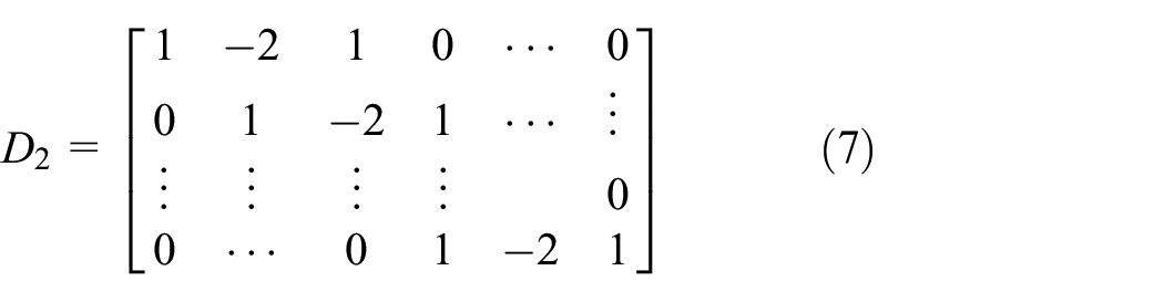
In Formula (8), the action of matrix L is equivalent to a high-pass filter. By performing Fourier transform on any row of the matrix L, its frequency characteristics can be obtained. Take N = 50, λ = 50, and use MATLAB to calculate according to Formula (6) and Formula (7). The frequency response of L is shown in Figure 1.

Figure 1.

Frequency response of L.

In Figure 1, the x-axis is the normalized frequency f, and the z-axis represents the amplitude. Due to the principle of symmetry, N in the y-axis only takes the data between 1 and 25. It can be seen from Figure 1 that the filtering effect of L is mostly smooth, the filtering effect is not ideal only in the initial and final stages of the signal. It can be found that there is obvious attenuation in the low frequency band of the time-varying frequency characteristic curve. Let the regularization parameter λ take different values and perform the Fourier transform on the N/2th line of L to obtain the frequency response corresponding to different λ values. The results are shown in Figure 2. It is calculated that when λ is equal to 1, 2,5, 50, and 200, the corresponding cut-off frequencies are respectively 0.189, 0.132, 0.090, 0.041, and 0.011 times the sampling frequency. As the regularization paramete λ gradually increases, its relative cutoff frequency becomes lower and lower.

Figure 2.

Frequency response at different λ.

Fuzzy entropy feature extraction

The SPA method in Section 2.1 is used to realize the multi-scale decomposition of the vibration signal of the rolling bearing, and obtain the distinguished characteristic between the trend item and the de-trend item. Calculate the fuzzy entropy (FE) value of the trend item and the de-trend item separately to determine the feature vector.

FE relies on the concept of fuzzy function and chooses the index function ${\mathrm{e}}^{-{(d/r)}^{\mathrm{n}}}$ as a fuzzy function to measure the similarity between two vectors. The exponential function ${\mathrm{e}}^{-{(d/r)}^{\mathrm{n}}}$ has the following characteristics ²¹ :

1. The continuity guarantees that its function value will not change suddenly.

2. The convex properties of the function ensure the maximum self-similarity of the vector itself.

For x(i) is a time series of length N, the FE is defined as follows:

• (1) Define m-dimensional vectors in order

$$X_{\mathrm{i}}^m=\{x(i),x(i+1),\cdots ,x(i+m-1)\}-\{x_0(i)\}$$

(9)

Where i = 1, 2, …, N-m+ 1. $X_{\mathrm{i}}^m$ is the value of x (i) from the continuous m starting at the ith point, with the mean x₀ (i) removed, $X_{\mathrm{i}}^m$ is the value of x (i) with the average value x₀ (i) removed from successive m starting from the i-th point, and

$${\mathrm{x}}_0(i)=\frac{1}{m}\sum _{j=0}^{m-1}x(i+j)$$

(10)

• (2) Define the distance between $X_{\mathrm{i}}^m$ and $X_{\mathrm{j}}^m$ as the maximum value of the difference between the corresponding elements, that

$$\begin{array}{c}\multicolumn{1}{c}{{\mathrm{d}}_{\mathrm{ij}}^m=d[X_i^m,X_j^m]}\\ =\underset{k\in (0,m-1)}{max}\left\{|[x(i+k)-x_0(i)]-[x(j+k)-x_0(i)]|\right\}\hfill \\ i,j=1,2,\cdots ,N-m;i\ne j\hfill \end{array}$$

(11)

• (3) By defining the fuzzy function $\mu ({\mathrm{d}}_{\mathrm{ij}}^m,n,r)$ , the similarity $D_{\mathrm{ij}}^m$ between the vectors $X_{\mathrm{i}}^m$ and $X_{\mathrm{j}}^m$ is determined

$$D_{\mathrm{ij}}^m=\mu ({\mathrm{d}}_{\mathrm{ij}}^m,n,r)=e^{-{(d_{\mathrm{ij}}^m/r)}^n}$$

(12)

Where $\mu ({\mathrm{d}}_{\mathrm{ij}}^m,n,r)$ is the exponential function, n and r respectively represent the boundary gradient and width.

• (4) Define function

$${\varphi }^{\mathrm{m}}(n,r)=\frac{1}{N-m}\sum _{i=1}^{N-m}\left(\frac{1}{N-m-1}\sum _{N-m}{D}_{\mathrm{ij}}^m\right)$$

(13)

• (5) Perform m+ 1 processing on the dimensions, and repeat steps (1) to (4),

$${\varphi }^{\mathrm{m}+1}(n,r)=\frac{1}{N-m}\sum _{i=1}^{N-m}\left(\frac{1}{N-m-1}\sum _{N-m}{D}_{\mathrm{ij}}^{m+1}\right)$$

(14)

• (6) When N is a finite length, the fuzzy entropy can be defined as

$$\mathrm{FE}(m,n,r,N)=\ln {\varphi }^m(n,r)-\ln {\varphi }^{m+1}(n,r)$$

(15)

Refer to literature ²² for the selection of the FE parameters in Formula (15). Consider that the greater the embedding dimension m, the longer the data length required, so choose m = 2, n determines the gradient of the similar tolerance boundary, the greater n, the greater the gradient, but it will cause the loss of detailed information, so choose n = 2, the similarity tolerance r represents the width of the fuzzy function boundary. If r is too large, statistical information will be lost. If r is too small, it will increase the sensitivity to the resulting noise, and the estimated statistical characteristics are not ideal. In this paper, refer to literature ²¹ and choose r = 0.15. In the selection of the SPA parameters, only the regularization parameter λ needs to be adjusted, the value of λ has certain adaptability, that is, the selection of λ between adjacent values has little effect on the overall decomposition effect. If the value of λ is too small, the extraction of trend items is more conservative. At this time, the difference between the trend item and the de-trend item is small, which will result in little difference in fuzzy entropy between the two components, reducing the separability between the states. When the value of λ is too large, the extraction of trend items is too aggressive, and the resulting trend items of different fault states are too stable, which also reduces the separability of each state. In this paper, λ = 5 is selected to perform the SPA decomposition on the original rolling bearing vibration signal in Dai et al. ¹⁹ After the FE extracts the vibration signal of the rolling bearing, the fault diagnosis of rolling bearing with different fault types can be realized.

Improved FSVM algorithm

The fuzzy support vector machine (FSVM) is an improvement on the traditional SVM. FSVM assigns a membership value (MBS)to each sample point. The size of the MBS value is determined according to the role of the sample point in classifying the construction of the hyperplane. Therefore, to create an FSVM model, it is necessary to construct a membership function (MBSF) and use this function to blur samples. ²³

Mathematical model of FSVM

Each sample point x_i corresponds to an MBS value s_i. In this way, to obtain a fuzzy training set $\mathrm{s}=\{(x_1,y_1,s_1),(x_2,y_2,s_2),\cdots ,(x_n,y_n,s_n)\}$ is different from the traditional training set, where ${\mathrm{x}}_i\in R^n$ , ${\mathrm{y}}_i\in \{-1,1\}$ , $0\le {\mathrm{s}}_i\le 1$ , then the optimal classification hyperplane after introducing the MBS value s_i in Formula (16) becomes the following optimization mathematical problem:

$$\min (\frac{1}{2}{w}^{T}w+C\sum _{i=1}^n{\xi }_i)$$

(16)

$$\{\begin{array}{c}\min \frac{1}{2}\Vert \omega {\Vert }^2+c\sum _{i=1}^n{s}_i{\xi }_i\hfill \\ \multicolumn{1}{c}{s.t.y_i(\omega ·x_i+b)\ge 1-{\xi }_i}\end{array}$$

(17)

Among them, in the above optimization mathematical model, the smaller s_i, the smaller the sample point corresponding to the role of the objective function, and the larger the converse. In order to solve the above problem, establish the Lagrange function:

$$\begin{array}{c}L(\omega ,b,\xi )=\frac{1}{2}\Vert \omega {\Vert }^2+c\sum _{i=1}^n{s}_i{\xi }_i\hfill \\ -\sum _{i=1}^n{\alpha }_i[y_i(\omega ·x_i+b)-1+{\xi }_i]-\sum _{i=1}^n{\beta }_i{\xi }_i\hfill \end{array}$$

(18)

Where, ${\alpha }_{\mathrm{i}},{\beta }_i\ge 0$ is lagrangian multiplier. ²⁴

At the saddle point, let the partial derivative of L for $\omega ,\mathrm{b}$ ,and $\xi$ is equal to 0, then,

$$\{\begin{array}{c}\frac{\partial L}{\partial \omega }=\omega -\sum _{\mathrm{i}=1}^n{\alpha }_i{y}_i{x}_i=0\hfill \\ \frac{\partial L}{\partial \mathrm{b}}=-\sum _{\mathrm{i}=1}^n{\alpha }_i{y}_i=0\hfill \\ \frac{\partial L}{\partial \xi }=c{s}_i-{\alpha }_i-{\beta }_i=0\hfill \end{array}$$

(19)

The Formula (19) is brought into the Formula (18), so that the problem of finding the optimal hyperplane in the Formula (18) is transformed into the quadratic programming problem of the following formula:

$$\{\begin{array}{c}\max \sum _{i=1}^n{\alpha }_i-\frac{1}{2}\sum _{i=1}^n\sum _{j=1}^n{\alpha }_i{\alpha }_j{y}_i{y}_j(x_i·x_j)\hfill \\ \multicolumn{1}{c}{s.t.\sum _{i=1}^n{\alpha }_i{y}_i=0c{s}_i\ge {\alpha }_i\ge 0i=1,2,\cdots ,n}\end{array}$$

(20)

At the same time, the optimal solution should also meet the following conditions:

$$\{\begin{array}{c}{\alpha }_{\mathrm{i}}\left[y_i(\omega ·x_i+b-1+{\xi }_i)\right]=0\hfill \\ \multicolumn{1}{c}{{\beta }_i{\xi }_i=(c{s}_i-{\alpha }_i){\xi }_i=0}\end{array}$$

(21)

In this way, the corresponding decision function can be obtained according to the input training set samples:

$$f\left(\mathrm{x}\right)=\mathrm{sgn}(\omega ·x+b)$$

(22)

It can be seen from the FSVM model that the sample ${\mathrm{x}}_i$ corresponding to ${\alpha }_{\mathrm{i}}=0$ is a correctly classified sample point, that is a non-support vector. The sample corresponding to $0\le {\alpha }_{\mathrm{i}}\le c{s}_i$ is a support vector in the ordinary sense. The sample points corresponding to ${\alpha }_{\mathrm{i}}=c{s}_i$ is a border support vector.

For the MBS with fixed parameter penalty coefficient c samples, ${\mathrm{s}}_i$ reflects the importance of the sample points. The greater the corresponding MBS, the smaller the probability of being misclassified. Therefore, in the construction of FSVM, The principle of making the MBS of noise or outlier points smaller and making the boundary support vector MBS larger should be followed.

Determination method of MBSF

It can be seen from the mathematical model of FSVM and SVM that the biggest difference between their algorithmic solutions is that FSVM has one more parameter than SVM, and this parameter is available for all sample points. This parameter is the corresponding MBS of the sample. The MBS is obtained by the MBSF calculating the characteristics of the samples. The samples corresponding to different spatial positions and different feature vectors have different MBS. Therefore, the quality of the MBSF structure, whether it is reasonable, whether it is difficult, or not, directly affects the quality, rationality, and difficulty of the corresponding FSVM algorithm. So, the structure of MBSF is designed by integrating many aspects. According to the different purposes of MBSF design, it is divided into two categories: one is to improve the classification effect, and the other is to solve the classification problem of fuzzy information in the data set.

There are two initial considerations when studying FSVM: one is to solve the problem that the generation of traditional SVM optimal classification hyperplane would be greatly affected by noise and outliers^25,26 points; another is that the data set we obtained in the actual problem may contain fuzzy information, so that SVM cannot classify it. ²⁷ Therefore, according to the purpose of introducing MBSF, the fuzzy MBSF can be divided into two categories: one is by introducing the fuzzy MBSF, the independent variable of the function is each training sample, considering the spatial distribution characteristics of the sample in the sample set, it is assigned to MBS, so that all training samples will get the MBS, according to the difference of MBS, the importance of the sample can be determined, so as to solve the characteristics of SVM’s sensitivity to noise and outliers to a certain extent; another is to indicate the subordinate probability of the sample to this category. If the probability of a sample belonging to the positive category is 0.7, then the MBS of the sample in the positive category sample set is 0.7, and the MBS in the negative category sample set is 0.3. In this paper, only the first MBSF determination method is studied, that is, introducing the MBSF to improve the classification efficiency of FSVM.

MBSF is generally designed as a function of a particular “location” distance from the sample to the data set. According to this special “different location,” it can be divided into two categories: MBSF based on the design of distance between sample and class center (DSC) and distance between sample and class center hyperplane (DSCH). The basic idea of the first MBSF design: First, the class center corresponding to the training set samples is obtained according to the clustering algorithm, and then, in the high-dimensional space, the distance of each sample to the corresponding class center is calculated by the idea of kernel function, ²⁸ and the MBSF is designed as an inverse function of the distance to the class center. The basic idea of the second MBSF design: First, the class center corresponding to the training set samples is also obtained according to the clustering algorithm, and secondly, two hyperplanes that pass through the class center and are perpendicular to each other (there are only one pair). Then, in the high-dimensional space, the distance of each sample to the corresponding DSCH is calculated with the help of the kernel function. Finally, the MBSF is designed as an inverse ratio function to the DSCH.

The FSVM designed based on the DCS is the first proposed algorithm to be widely used because of its simple and easy operation. However, designing the MBSF in this way will inevitably lead to different sizes of the support vectors and affect the classification accuracy. Although the FSVM algorithm designed based on DSCH can solve the above problems to a certain extent, the algorithm based on DSCH has a relatively high time complexity due to the calculation of DSCH, and the mandatory use of DSCH to reflect the poor generality of the MBS algorithm.

The adjustment factors is introduced in this paper after analyzing the potential support vector samples (PSVS), so that the class center is adjusted along the direction near the classification hyperplane. In this way, based on the adjusted class center, the DSCH-based FSVM model is used to obtain the self-adjusting FSVM algorithm in this paper. The improved algorithm obtained in this way can synthesize the advantages of the traditional model without incurring a large time cost.

The flow of the self-adjusting FSVM algorithm based on DSCH is as follows:

• (1) Divide the training samples into two categories: the positive and negative samples, respectively

$$\{\begin{array}{c}{c}^{+}=\left\{x_i|x_i\in c,y_i=1\right\}\hfill \\ \multicolumn{1}{c}{c^{-}=\left\{x_j|x_j\in c,y_j=-1\right\}}\end{array}$$

(23)

• (2) Determine the class center and the vector of class centers

$$\begin{array}{c}\mathrm{\Phi }\left({\mathrm{o}}_{+}\right)=\frac{1}{m}\sum _{i=1}^m\mathrm{\Phi }\left(x_i\right),m\mathrm{is}\mathrm{the}\mathrm{number}\mathrm{of}\mathrm{the}\mathrm{positive}\mathrm{samples}\hfill \\ \mathrm{\Phi }\left({\mathrm{o}}_{-}\right)=\frac{1}{n}\sum _{i=1}^n\mathrm{\Phi }\left(x_j\right),n\mathrm{is}\mathrm{the}\mathrm{number}\mathrm{of}\mathrm{the}\mathrm{negative}\mathrm{samples}\hfill \end{array}$$

(24)

$$\mathrm{\Phi }\left(\tilde{w}\right)=\mathrm{\Phi }\left({\mathrm{x}}_{+}\right)-\mathrm{\Phi }\left(x_{-}\right)$$

(25)

(3) Determine the DSCH: H1 and H2

$$\{\begin{array}{c}H1\perp \mathrm{\Phi }\left(\tilde{\mathrm{w}}\right)\\ H2\perp \mathrm{\Phi }\left(\tilde{\mathrm{w}}\right)\end{array}\mathrm{H}1\mathrm{and}H2\mathrm{passes}\mathrm{\Phi }\left({\mathrm{o}}_{+}\right)and\mathrm{\Phi }\left({\mathrm{o}}_{-}\right)\mathrm{respectively}$$

(26)

• (4) Calculate the $T_{+}$ and $T_{-}$ of the PSVS, and the average of their distances to their respective hyperplanes

$$\begin{array}{c}\multicolumn{1}{c}{D_{T_{+}}=(\mathrm{\Phi }\left({\mathrm{x}}_{+}\right)-\mathrm{\Phi }\left({\mathrm{x}}_{-}\right))·(\mathrm{\Phi }\left({\mathrm{x}}_{+}\right)-\mathrm{\Phi }\left({\mathrm{T}}_{+}\right))}\\ =\frac{1}{n_{+}^2}\sum _{i=1}^{n_{+}}\sum _{j=1}^{n_{+}}K(x_i,{\mathrm{x}}_{\mathrm{j}})+\frac{1}{n_{-}}\sum _{i=1}^{n_{-}}K(T_{+},{\mathrm{x}}_{-})\hfill \\ -\frac{1}{n_{+}}\sum _{i=1}^{n_{+}}K(T_{+},{\mathrm{x}}_{+})-\frac{1}{n_{+}\times n_{-}}\sum _{i=1}^{n_{+}}\sum _{j=1}^{n_{-}}K(x_i,{\mathrm{x}}_{\mathrm{j}})\hfill \end{array}$$

(27)

$$\begin{array}{c}\multicolumn{1}{c}{D_{T_{-}}=(\mathrm{\Phi }\left({\mathrm{x}}_{+}\right)-\mathrm{\Phi }\left({\mathrm{x}}_{-}\right))·(\mathrm{\Phi }\left({\mathrm{x}}_{-}\right)-\mathrm{\Phi }\left({\mathrm{T}}_{-}\right))}\\ =\frac{1}{n_{+}\times n_{-}}\sum _{i=1}^{n_{+}}\sum _{j=1}^{n_{-}}K(x_i,{\mathrm{x}}_{\mathrm{j}})-\frac{1}{n_{+}}\sum _{i=1}^{n_{+}}K(T_{-},{\mathrm{x}}_{+})\hfill \\ -\frac{1}{n_{-}^2}\sum _{i=1}^{n_{-}}\sum _{j=1}^{n_{-}}K(x_i,{\mathrm{x}}_{\mathrm{j}})+\frac{1}{n_{-}}\sum _{i=1}^{n_{-}}K(T_{-},{\mathrm{x}}_{-})\hfill \end{array}$$

(28)

$$\begin{array}{c}{\mathrm{d}}_{T_{+}}=\frac{1}{n_{T_{+}}}\sum _{i=1}^{n_{T_{+}}}\left|D_{T_i}\right|\hfill \\ {\mathrm{d}}_{T-}=\frac{1}{n_{T-}}\sum _{i=1}^{n_{T-}}\left|D_{T_i}\right|\hfill \end{array}$$

(29)

• (5) The adjustment factor is calculated according to the PSVS and offset proportional coefficient

$$\begin{array}{c}{\mathrm{d}}_{+}=K_1*d_{T_{+}}{K}_1\ge 0\hfill \\ {\mathrm{d}}_{-}=K_2*d_{T_{-}}{K}_2\ge 0\hfill \end{array}$$

(30)

• (6) The adjusted class centers are obtained by the adjustment factors

$$\begin{array}{c}\mathrm{\Phi }{\left({\mathrm{x}}_{+}\right)}^{\prime }=\frac{(\mathrm{\Phi }\left(x_{-}\right)-\mathrm{\Phi }\left(x_{+}\right))\times d_{+}}{D}+\mathrm{\Phi }\left(x_{+}\right)\hfill \\ \mathrm{\Phi }{\left({\mathrm{x}}_{-}\right)}^{\prime }=\frac{(\mathrm{\Phi }\left(x_{+}\right)-\mathrm{\Phi }\left(x_{-}\right))\times d_{-}}{D}+\mathrm{\Phi }\left(x_{-}\right)\hfill \end{array}$$

(31)

• (7) According to the distance $D_{T_{\mathrm{i}}}$ from the sample to the class center, calculate the distance $D_{T_{\mathrm{i}}}^{\prime }$ from the sample to the adjusted DSCH

$$\begin{array}{c}{D}_{T_{\mathrm{i}+}}^{\prime }=\{\begin{array}{c}{D}_{T_{\mathrm{i}+}}-d_{+}{D}_{T_{\mathrm{i}+}}>d_{+}\mathrm{and}\mathrm{the}\mathrm{samples}\mathrm{are}\mathrm{potential}\mathrm{support}\mathrm{vector}\mathrm{sample}\mathrm{points}\hfill \\ \multicolumn{1}{c}{d_{+}-D_{T_{\mathrm{i}+}}{D}_{T_{\mathrm{i}+}}<d_{+}\mathrm{and}\mathrm{the}\mathrm{samples}\mathrm{are}\mathrm{potential}\mathrm{support}\mathrm{vector}\mathrm{sample}\mathrm{points}}\\ \multicolumn{1}{c}{D_{T_{\mathrm{i}+}}+d_{+}\mathrm{the}\mathrm{samples}\mathrm{are}\mathrm{not}\mathrm{potential}\mathrm{support}\mathrm{vector}\mathrm{sample}\mathrm{points}}\end{array}\hfill \\ D_{T_{\mathrm{i}-}}^{\prime }=\{\begin{array}{c}{D}_{T_{\mathrm{i}-}}-d_{-}{D}_{T_{\mathrm{i}-}}>d_{-}\mathrm{and}\mathrm{the}\mathrm{samples}\mathrm{are}\mathrm{potential}\mathrm{support}\mathrm{vector}\mathrm{sample}\mathrm{points}\hfill \\ \multicolumn{1}{c}{d_{-}-D_{T_{\mathrm{i}-}}{D}_{T_{\mathrm{i}-}}<d_{-}\mathrm{and}\mathrm{the}\mathrm{samples}\mathrm{are}\mathrm{potential}\mathrm{support}\mathrm{vector}\mathrm{sample}\mathrm{points}}\\ \multicolumn{1}{c}{D_{T_{\mathrm{i}-}}+d_{-}\mathrm{the}\mathrm{samples}\mathrm{are}\mathrm{not}\mathrm{potential}\mathrm{support}\mathrm{vector}\mathrm{sample}\mathrm{points}}\end{array}\hfill \end{array}$$

(32)

• (8) Using DSCH algorithm to construct MBSF

$$\begin{array}{c}\mathrm{s}\left(i_{+}\right)=\{\begin{array}{c}1-\frac{d_{i_{+}}}{max\left(d_{i_{+}}\right)+\delta }{d}_{i_{+}}\le (d_{+}+\frac{1}{2}max\left(d_{i_{+}}\right))\hfill \\ \multicolumn{1}{c}{\epsilon d_{i_{+}}>(d_{+}+\frac{1}{2}max\left(d_{i_{+}}\right))}\end{array}\hfill \\ \mathrm{s}\left(i_{-}\right)=\{\begin{array}{c}1-\frac{d_{i_{-}}}{max\left(d_{i_{-}}\right)+\delta }{d}_{i_{-}}\le (d_{-}+\frac{1}{2}max\left(d_{i_{-}}\right))\hfill \\ \multicolumn{1}{c}{\epsilon d_{i_{-}}>(d_{-}+\frac{1}{2}max\left(d_{i_{-}}\right))}\end{array}\hfill \end{array}$$

(33)

Among them, s is the MBS of the sample, ${\mathrm{d}}_{i_{+}}$ and ${\mathrm{d}}_{i_{-}}$ are the distances of the positive and negative samples to the adjusted DSCH respectively, ε is a small positive number for the isolated MBS, ${\mathrm{d}}_{i_{+}}$ and ${\mathrm{d}}_{i_{-}}$ are the adjustment factors of the positive and negative samples respectively and very small positive numbers. It can be seen that by defining the adjustment factor, the class center moves along the direction of the support vector, increasing the gap of the MBS values between the support vector and the noise and outlier points. The adjustment factor is introduced to solve the dependence of traditional FSVM on the spherical distribution of the sample points to a certain extent. The adjustment factor is relatively small for the data set with a relatively concentrated sample distribution, and the adjustment factor is relatively large for the data set with a relatively scattered sample distribution. With the setting of s, the points near the classification hyperplane that cannot be support vectors have smaller MBS. The offset scale factor is defined to control the size of the distance from the class center. In particular, when the scale factor is K = 0, the algorithm in this paper is equivalent to the traditional FSVM based on the DSCH.

We selected four UCI datasets of Cancer dataset, German dataset, Liver dataset and Vote dataset for IFSVM experiment analysis, and used linear kernel function and gaussian kernel function to carry out traditional FSVM (TFSVM) and IFSVM on the above four datasets. When a linear kernel function was used, the penalty coefficient C was sampled in a continuous range to obtain a certain amount of C. The different penalty coefficients C were used for the data sets, the classification accuracy obtained by the two algorithms is compared. When using the gaussian kernel function, the penalty coefficient C and the kernel parameter K were sampled in different continuous ranges to obtain a certain number of C and K, and then the classification accuracy corresponding to C and K was obtained in different data sets. Here we compared the average accuracy of the classifications obtained with different penalty coefficients C under the same kernel function, and compared the average accuracy of the classification under different kernel parameters. This paper only lists the comparison analysis charts of the TFSVM and IFSVM methods of the vote data set, as shown in Figures 3 and 4. It can be seen from Figures 3 and 4 that the IFSVM algorithm of this paper performs better than TFSVM in most of the kernel parameter intervals for all the data sets.

Figure 3.

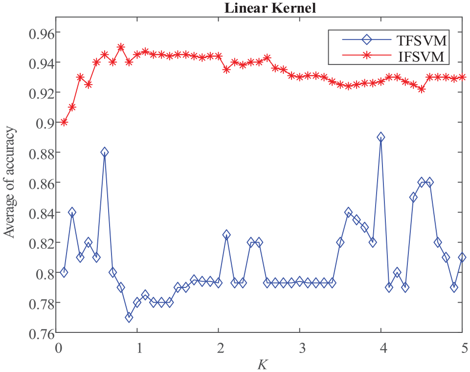
Comparison analysis charts of the TFSVM and IFSVM methods of the vote data set in Linear Kernel.

Figure 4.

Comparison analysis charts of the TFSVM and IFSVM methods of the vote data set in Gaussian Kernel.

Fault diagnosis method of rolling bearing based on SPA-FE-IFSVM

Procedure of the fault diagnosis method

The fault diagnosis method of rolling bearing based on SPA-FE-IFSVM proposed in this paper is as follows:

• (1) The original rolling bearing vibration signals in different states are decomposed by SPA to obtain the corresponding trend items and de-trend items as the components containing the main fault information of the rolling bearing.

• (2) According to the FE parameters set in Section 2.2 of this paper, the FE values of the trend and de-trend terms for the rolling bearing vibration signals in different states are calculated as the eigenvector T of the rolling bearing fault diagnosis.

$$T=\left[\begin{array}{c}{\mathrm{FE}}_{\mathrm{trend}}^1,{\mathrm{FE}}_{\mathrm{de}-\mathrm{trend}}^1\hfill \\ \multicolumn{1}{c}{{\mathrm{FE}}_{\mathrm{trend}}^2,{\mathrm{FE}}_{\mathrm{de}-\mathrm{trend}}^2}\\ \multicolumn{1}{c}{⋮⋮}\\ \multicolumn{1}{c}{{\mathrm{FE}}_{\mathrm{trend}}^n,{\mathrm{FE}}_{\mathrm{de}-\mathrm{trend}}^n}\end{array}\right]$$

(34)

• (3) The eigenvector value obtained by Formula (34) is input into the IFSVM classifier to obtain the fault classification result and realize the rolling bearing fault diagnosis.

The flow chart of the rolling bearing fault diagnosis method based on SPA-FE-IFSVM is shown in Figure 5.

Figure 5.

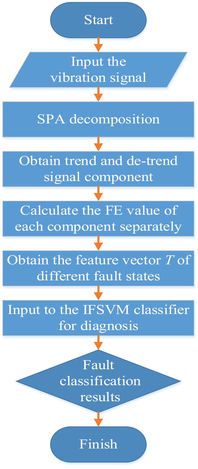
Flow chart of the rolling bearing fault diagnosis method based on SPA-FE-IFSVM.

Experimental analysis

In order to verify the validity and accuracy of the SPA-FE-IFSVM method proposed in this paper, the data of 6205-2RS JEM SKF deep groove ball bearings in the rolling bearing experiment of Western Reserve University was selected as the verification data. ⁵ The motor load is 735.5W and the bearing speed is 1772r/min. The fault is arranged by electric spark technology, the fault diameter is 0.355 6 mm, and the fault depth is 0.279 4 mm. The sampling frequency of the vibration signals in four states is 12 kHz. The length of the selected data sample is 2048. In addition to the normal state (NORM), the three fault states are respectively recorded as rolling element fault (REF), inner race fault (IRF) and outer race fault (ORF). The vibration acceleration signal of the rolling bearing in four states is shown in Figure 6.

Figure 6.

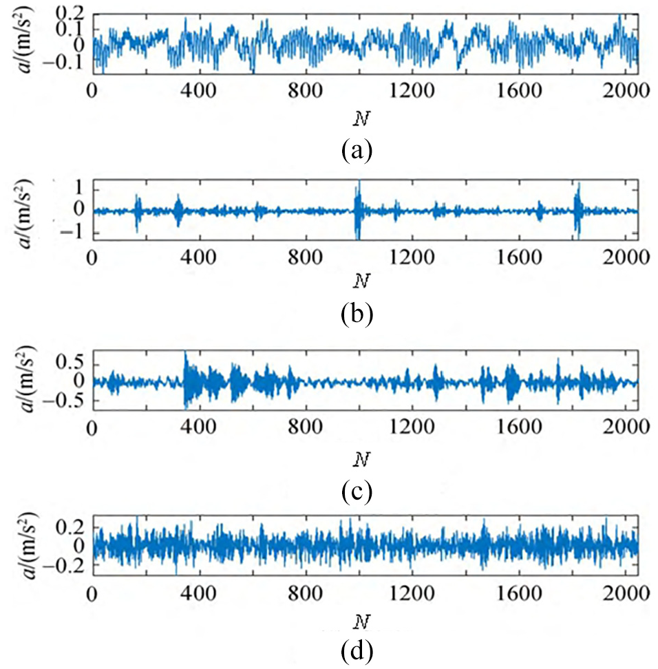
Vibration acceleration signals of rolling bearings in four states: (a) NORM, (b) REF, (c) IRF, and (d) ORF.

Select 80 groups of samples in four states: NORM, REF, IRF, and ORF. In the fault diagnosis process, 40 sets of each state data are selected as the training set, and the remaining 40 sets are used as the test set to verify the effectiveness of the algorithm.

First, the vibration signal of rolling bearing is decomposed by SPA. Taking the vibration signal in the normal state as an example, according to the initial conditions set in Section 2.2 of this paper, the SPA decomposition result under λ = 5 is obtained, as shown in Figure 7. It can be seen from Figure 7 that after SPA decomposition, the resulting trend items are clearly distinguished from the de-trend items, and the trend items retain the basic trend characteristics and physical characteristics of the original signal, proving that the SPA method performs the rationality of scale decomposition. The running time of the SPA method in Figure 7 is 0.09 s. The algorithm is extremely simple and fast.

Figure 7.

Trend items and de-trend items of SPA for the NORM vibration signal: (a) NORM, (b) trend items, and (c) de-trend items.

For comparative analysis, the vibration signal of the NORM is also decomposed by EMD. After EMD decomposition, 10 IMF components and 1 trend item are obtained, and the number of components obtained is much larger than that of SPA decomposition. Only the first four IMF components are selected for display, as shown in Figure 8. Compared with SPA decomposition, the difference between adjacent components in the IMF components obtained by EMD is lower. In the subsequent feature extraction process, the difference between the feature quantities corresponding to each component is lower than SPA decomposition. In order to verify the ability of the SPA-FE algorithm to extract the feature vector of the rolling bearing fault signal, all samples collected were first decomposed by SPA, and then the obtained the FE values of trend items and detrend items, the corresponding results are shown in Figure 9.

Figure 8.

First four IMF components of EMD for the NORM vibration signal.

Figure 9.

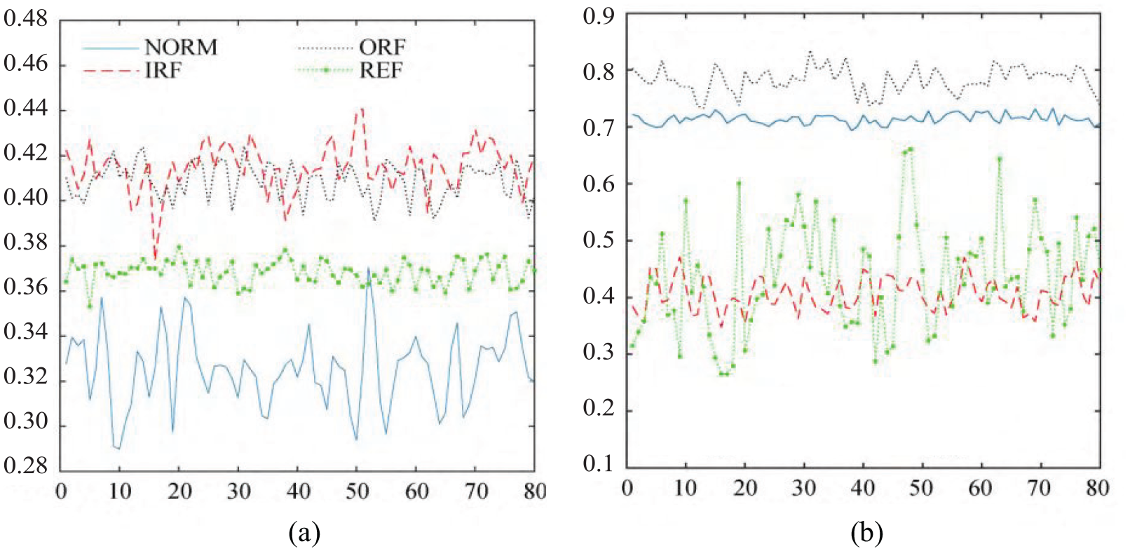
FE values of trend items and de-trend items:

The FE value of the trend item is low in Figure 9. In numerical form, a good distinction is made between the NORM and the REF, but there is a certain degree of overlap between the IRF and the ORF. If the IFSVM classification is directly performed, it will easily cause misjudgment. So the FE value of the trend item is taken as the eigenvector 1, which is recorded as ${\mathrm{FE}}_{\mathrm{trend}}^{\lambda =5}$ .Compared with the trend item, the de-trend item has a significantly greater value than the trend item in Figure 9. This is because the time series of the de-trend item is more complex than the trend item, and it is also reflected in Figure 7. The FE value of the trend item can effectively distinguish the NORM from the ORF, but there is an overlap between the IRF and the REF. It can be seen from the analysis in Figure 9 that the FE value of the de-trend item is taken as the eigenvector 2 and recorded as ${\mathrm{FE}}_{\mathrm{de}-\mathrm{trend}}^{\lambda =5}$ , combining trend item and de-trend item to form the eigenvector, which can completely summarize the fault information. Set label 1 (L₁), label 2 (L₂), label 3 (L₃), label 4 (L₄) to correspond to the NORM, the IRF, the REF, and the ORF, respectively. Construct the IFSVM input format of each sample

$$T=[{\mathrm{FE}}_{\mathrm{trend}}^{\lambda =5},{\mathrm{FE}}_{\mathrm{de}-\mathrm{trend}}^{\lambda =5},L_i]$$

(35)

It can be known from Formula (35) that the eigenvector of the rolling bearing based on SPA-FE contains only two feature information, which simplifies the calculation process and improves the adaptability of the eigenvector selection.

The above-mentioned SPA-FE analysis is performed on 80 groups of NORM, REF, IRF and ORF samples, and the state label is marked, and then the above eigenvectors are input into the IFSVM classifier for failure state recognition as shown in Table 1. Table 1 shows that the SPA-FE-IFSVM-based method of this paper has a higher fault diagnosis rate. In order to verify the superiority of this method, the same data samples are selected, and the fault diagnosis of FE-SVM method, EMD-FE-SVM method, SPA-FE-SVM and SPA-FE-IFSVM method is also shown in Table 1.

Table 1.

Recognition accuracy of all fault diagnosis methods.

Fault diagnosis method	Recognition accuracy (%)				Total accuracy (%)
	NORM	REF	IRF	ORF
SPA-FE-IFSVM	100	97.5	97.5	97.5	98.125
SPA-FE-SVM	95	95	92.5	92.5	93.75
EMD-FE-SVM	90	87.5	90	87.5	88.75
FE-SVM	82.5	80	80	82.5	81.25

The results show that both the accuracy in each state and the total accuracy of the proposed method are better than those of three other fault diagnosis methods under the condition of the same finite number of samples. Feature vectors extracted by SPA-FE are better than those achieved by EMD-FE and only FE method from the result of recognition rate, so it is necessary to combine the self-decomposition method with FE for resisting noise interference and highlighted information extraction, while SPA is a superior method than EMD for these fault vibration signals according to the better recognition rate. From Table 1, we also see that the fault recognition rates of EMD-FE-SVM are lower than that of the proposed method, it demonstrates the superiority of the IFSVM method over SVM in the accuracy of fault identification. Through the comparative researches above, we know that the proposed method is a superior fault diagnosis method to diagnosis faults of reciprocating compressor valve effectively and accurately.

Conclusion

This paper presents a fault diagnosis method based on SPA-FE and IFSVM, and it is applied for the fault diagnosis of rolling bearing.

1. In the proposed method, the SPA decomposition can effectively separate the trend item and de-trend item of the original signal, and summarize the characteristic information of the original vibration signal at two scales, which effectively improves the accuracy of fault diagnosis. The number of variables obtained by SPA decomposition is less, and the degree of discrimination is higher, which avoids the selection of excessive feature quantities in traditional multi-scale decomposition and effectively improves the efficiency and speed of fault diagnosis.

2. A FE method was utilize to characterize the trend item and de-trend item components, and extract the FE values to construct the eigenvectors, which can solve the problem of describing the fuzzy edge of the sample datas, and accurately extract fault information.

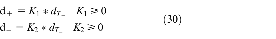
3. According to SVM is unable to deal with fuzzy information and the characteristics of the sensitivity to noise, on the basis of FSVM, a self-adjusting IFSVM algorithm based on PSVS analysis using DSCH is proposed. By analyzing the PSVS data, the class center offset factor is obtained. Adjusting the offset factor and an offset scale factor causes the class center to move in the direction of the classification hyperplane, which makes the data sets have better adaptability, improves the generalization ability of the algorithm, and achieves better classification accuracy.

4. This method was applied for the rolling bearing at different states, and the effectiveness of this method is verified by the recognition results compare to other fault diagnosis methods.