Intelligent batch process method for analyzing the effect of the suspension parameters on the vibration of the suspended monorail

Abstract

As for the batch process, it is needed to carry out a unique simulation for each group of parameters. The simplest method to achieve this goal is to uses the Simulink as the integration space. It cannot solve some complicated dynamic model set up in dynamic software. This paper introduces an intelligent batch program to enable the model solved in the dynamic software during the simulation. This paper also put forward the road equation for the suspended monorail, which has not been introduced before. The results of multi rigid body dynamics and vehicle bridge coupling dynamics are compared in this paper. It proves that the bridge vibration has little effect on the vehicle system. Through the batch process method, the effect of different parameters on the vehicle system could be obtained.

Introduction

The study of monorail dynamics focus on five aspects^1,2: (1) vehicle model, (2) bridge model, (3) road excitation, (4) wheel rail contact relationship, and (5) calculation method.

At present, the multi rigid body method^2–13 is used to set the vehicle model. The vehicle system is simplified as a multi rigid body system composed of multiple spring and damping elements, and the vibration differential equation is obtained by D’Alembert’s principle. Liu ² also pointed out that the vibration equation of straddle type monorail is similar to that of the railway vehicle.^14,15

The modeling methods of monorail dynamics mainly include multi rigid body dynamics and vehicle bridge coupling dynamics. The multi rigid body dynamics of vehicle does not consider the deformation of track beam, and the excitation of vehicle system is provided by the road irregularities. This method is used in reference Kenjiro et al., Wen, Gabriel and Roberto, and Goda et al.^6,7,11,16 For the suspended monorail, the flexible deformation of the track beam is larger than that of the straddle type one. In order to obtain better simulation accuracy, the finite element modeling of the track beam is usually needed. However, in certain cases, when only wheel eccentricity is considered, ¹⁷ the track beam is not modeled. In addition, in some calculations that pay more attention to the vehicle characteristics, the track beam can also be regarded as rigid body.^18,19

When the deformation of the track beam is needed to be considered, the modeling of the track beam becomes necessary. One method is to set the finite element model of the track beam first. Then import it into the dynamics software to couple with the multi rigid body model of the vehicle.^2–5,7–10 At present, this method is often used in the dynamic method of the suspended monorail when the vibration of track beam is considered.^20–22 Some domestic researches also analyze the vehicle bridge coupling dynamics.^23,24 Reference Meysam et al. ⁹ specifically carries out the finite element modeling of the stiffener on the track beam, and compares it with that of no stiffeners. ⁴ Another method is to establish the finite element model of track beam first. Then set the spatial motion equation of vehicle bridge coupling system, and use FORTRAN to solve it.^25,26

In reference Wang and Zhu, ¹² the finite element elements of track beam are divided into three types: steel beam element, concrete beam element, and shear connection element. Because the span of the track beam is much longer than the beam height, it can be simplified as the Euler beam model, ²⁷ which is also used in the reference Liu. ² In addition, considering the rigidity of the track beam and the flexible deformation of the connection components, the track beam can be modeled as a multi rigid body dynamic system connected by some spring damping elements ²⁸

However, there is no researches on the effect of the vehicle suspension parameters (namely stiffness and damping of the suspension system) on the suspended monorail systems. This paper is to analyze the effect of vehicle parameters. The simplest method to achieve this goal is to use the Simulink as the integration space. it cannot solve some complicated dynamic model set up in dynamic software. To solve the problem, this paper introduces an intelligent batch program to enable the model solved in the dynamic software during simulation.

Test verification for road irregularities

The exact values of road irregularities are verified through a monorail experiment in China. Using the simulated road irregularities, the simulated acceleration is closed to the experiment data. Then the formula of the simulated road irregularities is obtained. The acceleration sensors are mounted on the floor of the carriage, as shown in Figure 1.

Figure 1.

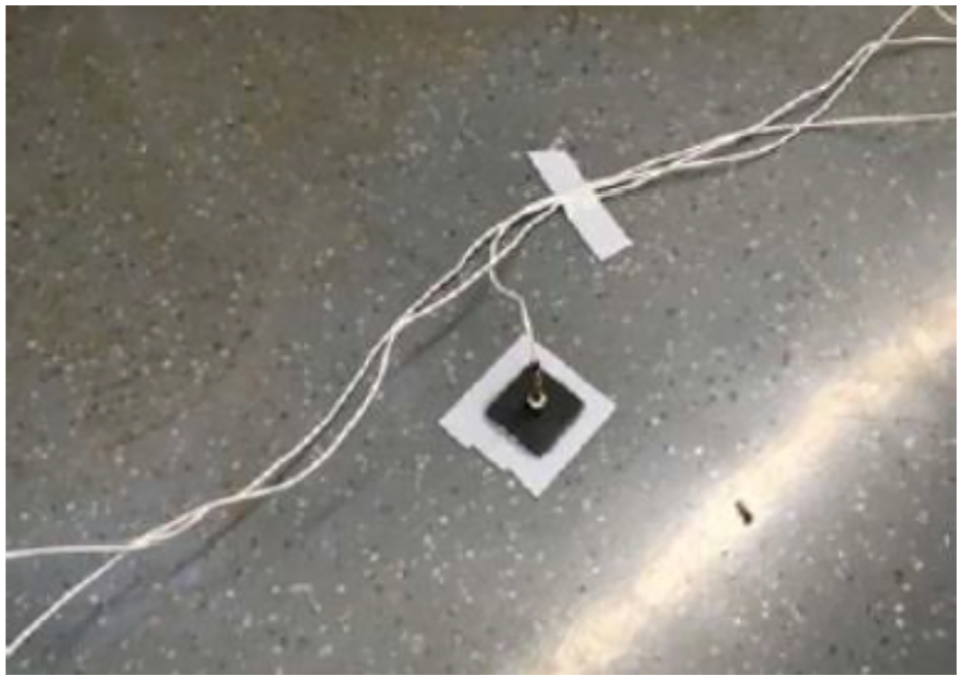
Arrangement of acceleration sensor.

He ²⁹ has compared the simulated result and the tested data of that monorail. It is known from Figure 2 that the amplitude of the test data is similar as the simulated result.

Figure 2.

Comparison between simulation result and test data: (a) lateral, (b) vertical. ²⁹

The road irregularities are generated through Monte Carlo method. As for straddle monorail, the following formula is concluded as follows:

$$\mathrm{S}\left(\mathrm{\Omega }\right)=\frac{\alpha }{{\mathrm{\Omega }}^n+{\beta }^n}$$

(1)

For the suspended monorail, this formula could also be used to build the PSD function, but the parameters need to be redefined. In this paper, “nlinfit” is used as the fitting strategy.

The Levenberg-Marquardt nonlinear least squares algorithm is used for nonrobust estimation.

Take ${\mathrm{\Omega }}_k$ as the No. k iterative point of $\mathrm{\Omega }$ . According to Taylor formula, the approximate value of $\mathrm{S}\left(\mathrm{\Omega }\right)$ could be defined as follows:

$$\mathrm{S}\left(\mathrm{\Omega }\right)=\mathrm{S}\left({\mathrm{\Omega }}_k\right)+\mathrm{J}\left({\mathrm{\Omega }}_k\right)(\mathrm{\Omega }-{\mathrm{\Omega }}_k)$$

(2)

$$\mathrm{J}\left({\mathrm{\Omega }}_k\right)=\left[\begin{array}{ccc}\frac{\partial S_1}{\partial {\mathrm{\Omega }}_1}\hfill & \dots \hfill & \frac{\partial S_1}{\partial {\mathrm{\Omega }}_n}\hfill \\ \multicolumn{1}{c}{⋮}& ⋮\hfill & ⋮\hfill \\ \multicolumn{1}{c}{\frac{\partial S_m}{\partial {\mathrm{\Omega }}_1}}& \dots \hfill & \frac{\partial S_1}{\partial {\mathrm{\Omega }}_n}\hfill \end{array}\right]$$

Then the trust region model is set up as follows

$$\{\begin{array}{c}min\left||\mathrm{S}\left({\mathrm{\Omega }}_k\right)+\mathrm{J}\left({\mathrm{\Omega }}_k\right)(\mathrm{\Omega }-{\mathrm{\Omega }}_k)|\right|\hfill \\ \multicolumn{1}{c}{s.t.\left||\mathrm{\Omega }-{\mathrm{\Omega }}_k\left||\le |\right|{\mathrm{\Delta }}_k|\right|}\end{array}$$

(3)

${\mathrm{\Delta }}_k$ denotes the radius of the trust region.

$$(\mathrm{J}{\left({\mathrm{\Omega }}_k\right)}^T\mathrm{J}\left({\mathrm{\Omega }}_k\right)+{\lambda }_{k}I)d=-\mathrm{J}{\left({\mathrm{\Omega }}_k\right)}^T\mathrm{S}\left({\mathrm{\Omega }}_k\right)$$

(4)

Then, The L-M direction formula can be obtained as follows.

$$d_k=-{(\mathrm{J}{\left({\mathrm{\Omega }}_k\right)}^T\mathrm{J}\left({\mathrm{\Omega }}_k\right)+{\lambda }_{k}I)}^{-1}\mathrm{J}{\left({\mathrm{\Omega }}_k\right)}^T\mathrm{S}\left({\mathrm{\Omega }}_k\right)$$

(5)

$d_k$ denotes the L-M direction. ${\lambda }_k\ge 0$ .

As for the robust estimation, the iterative reweighted least squares algorithm is used. In this algorithm, robust weights will be modified according to the observation’s residual from the previous iteration.

The fitting results are shown in Figure 3 and the fitting parameters of equation (1) are shown in Table 1. It is concluded that the irregularities of suspended monorail are much closer to the US level 6 rail irregularities.

Figure 3.

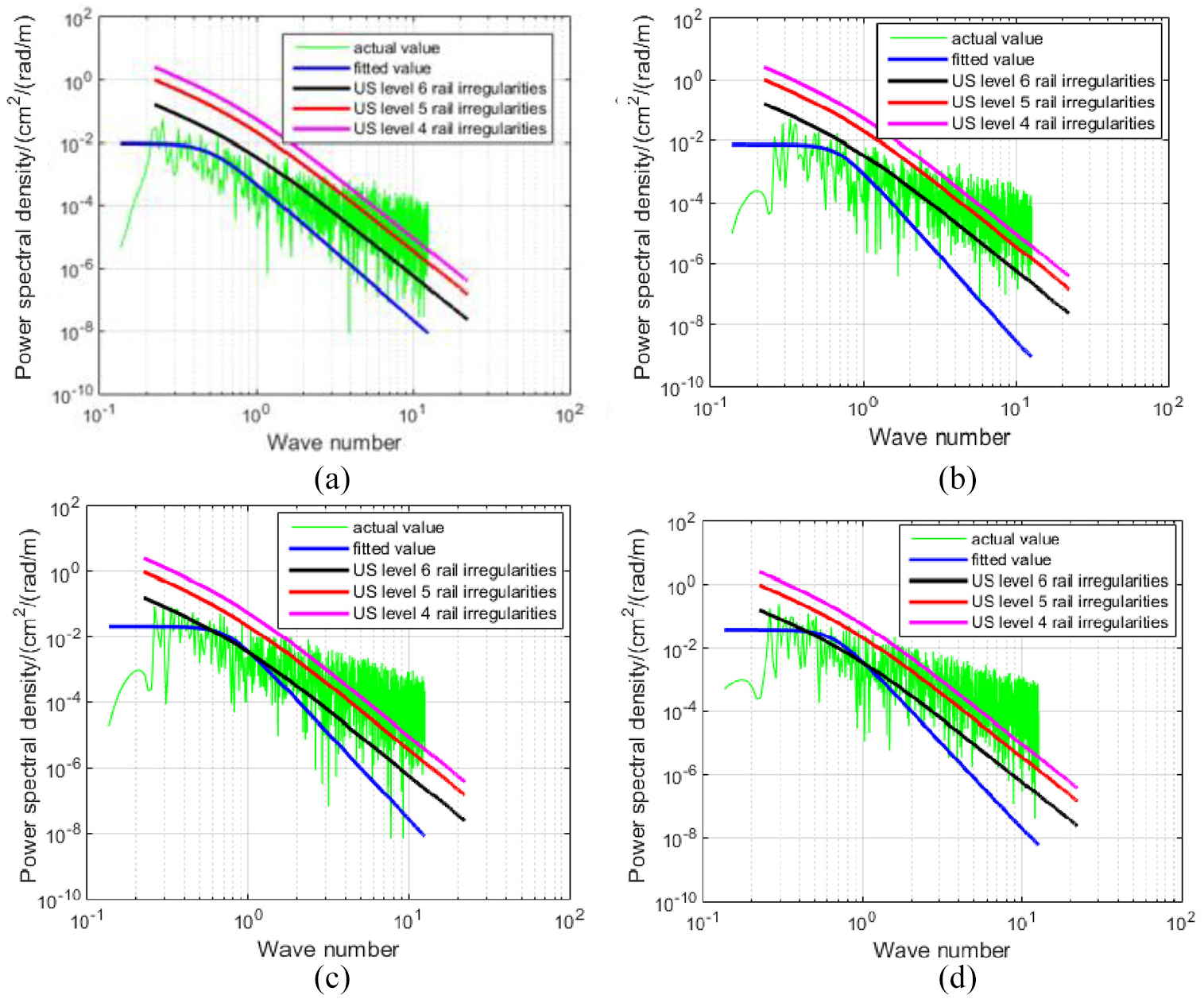
PSD figure of road irregularities: (a) left guide rail, (b) right guide rail, (c) left driving rail, (d) right driving rail.

Table 1.

Fitting parameter of the PSD function.

	α	β	n
Left guiding surface	0.00049	0.50588	4.33060
Right guiding surface	0.00097	0.68625	5.49330
Left driving surface	0.00429	0.73436	5.21134
Right driving surface	0.00394	0.65330	5.30192

Vehicle model

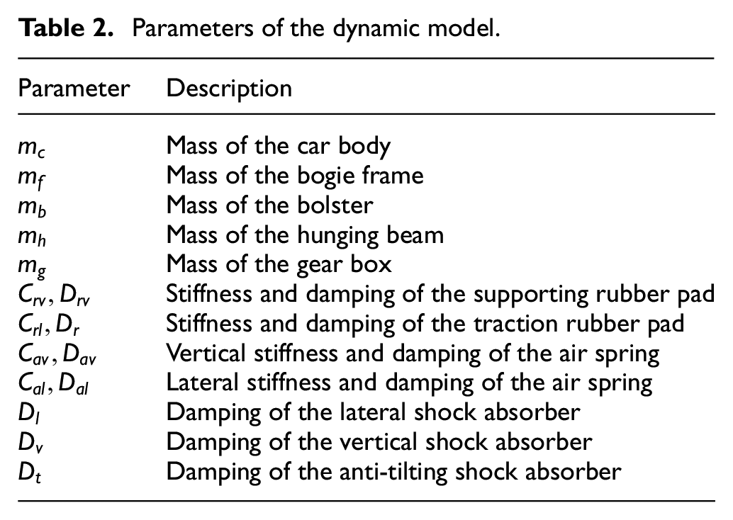
The dynamic model of the vehicle system is shown in Figure 4. Like most typical suspended monorails in the world, the bogie runs inside the box girder, and the car body suspends under it. As shown in Figure 5, the driving wheels, mounted on the gear box support the vehicle and drive it forward. There are traction rubber pad and supporting rubber pad between the gear box and bogie frame to alleviate the vibration. The guide wheels provide guidance for the bogie and the stable wheels prevent it overturning. There is a traction rod between the car body and bogie, which provides the traction power for the car body. There are hanging beams on the top of the car body, and the bolster suspended under them. The air springs, vertical shock absorbers, lateral shock absorbers play an important role as the secondary suspension. The lateral stops prevent the large vibration between them. There are anti-tilting shock absorbers and anti-tilting stops to prevent the severe tilting vibration of the bolster. The parameters are shown in Table 2.

Figure 4.

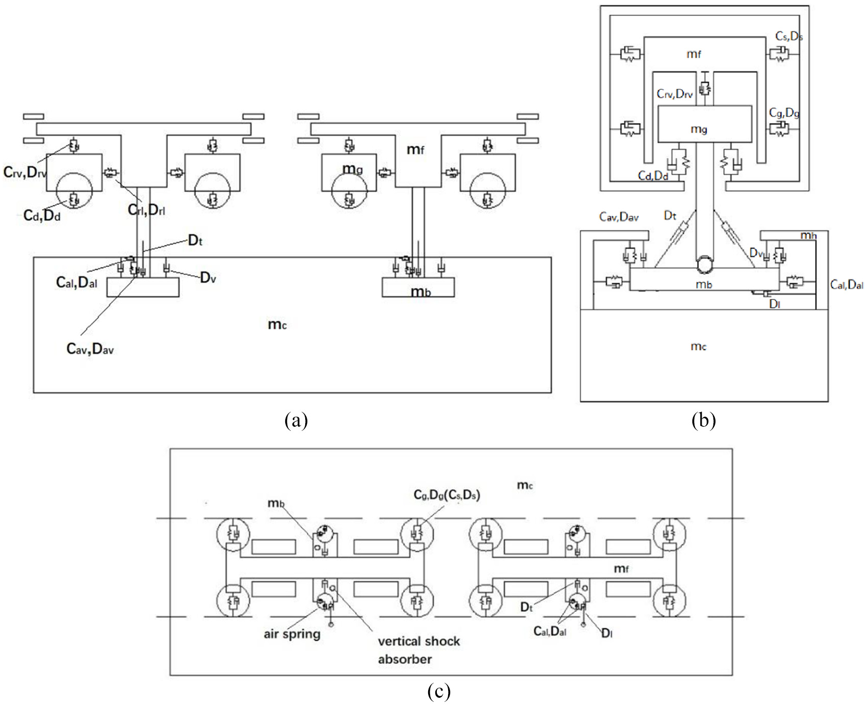
Dynamic model of the vehicle system: (a) right view; (b) front view; (c) top view.

Figure 5.

Bogie structure.

Table 2.

Parameters of the dynamic model.

Parameter	Description
$m_c$	Mass of the car body
$m_f$	Mass of the bogie frame
$m_b$	Mass of the bolster
$m_h$	Mass of the hunging beam
$m_g$	Mass of the gear box
$C_{\mathrm{rv}},D_{\mathrm{rv}}$	Stiffness and damping of the supporting rubber pad
$C_{\mathrm{rl}},D_r$	Stiffness and damping of the traction rubber pad
$C_{\mathrm{av}},D_{\mathrm{av}}$	Vertical stiffness and damping of the air spring
$C_{\mathrm{al}},D_{\mathrm{al}}$	Lateral stiffness and damping of the air spring
$D_l$	Damping of the lateral shock absorber
$D_v$	Damping of the vertical shock absorber
$D_t$	Damping of the anti-tilting shock absorber

The bogie structure is shown in Figure 5.

The topological graph of the vehicle system is shown in Figure 6.

Figure 6.

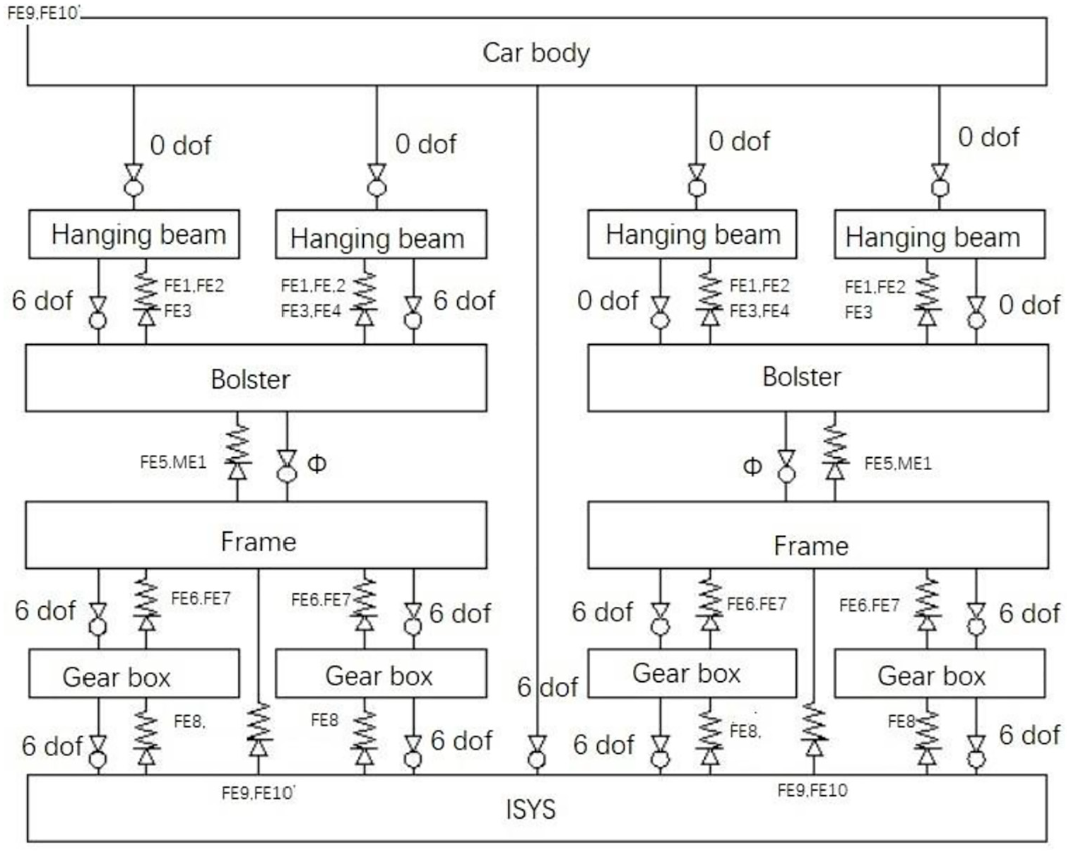
Topological graph of the vehicle system.

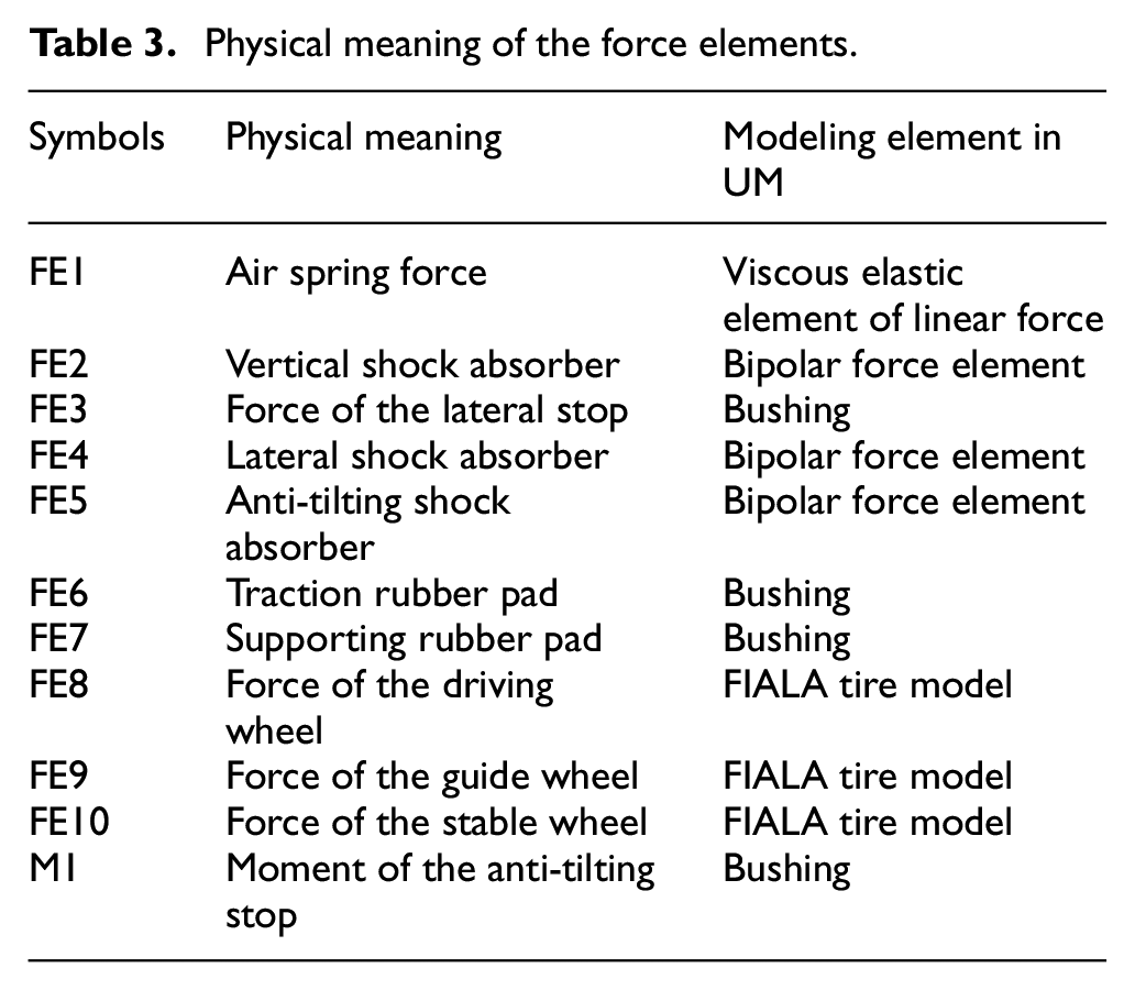
The physical meanings of the force elements are shown in Table 3, which are modeled by different model elements in UM (Universal Mechanism). The dynamic equations are in shown in the Supplemental Appendix.

Table 3.

Physical meaning of the force elements.

Symbols	Physical meaning	Modeling element in UM
FE1	Air spring force	Viscous elastic element of linear force
FE2	Vertical shock absorber	Bipolar force element
FE3	Force of the lateral stop	Bushing
FE4	Lateral shock absorber	Bipolar force element
FE5	Anti-tilting shock absorber	Bipolar force element
FE6	Traction rubber pad	Bushing
FE7	Supporting rubber pad	Bushing
FE8	Force of the driving wheel	FIALA tire model
FE9	Force of the guide wheel	FIALA tire model
FE10	Force of the stable wheel	FIALA tire model
M1	Moment of the anti-tilting stop	Bushing

Tire model

In many researches, the tire model is simplified as a spring element, which is not accurate at all. In this paper, the FIALA tire model is used to calculate the wheel force.

$$F_z=C_z\mathrm{\Delta }z+D_z\frac{\mathrm{d}\mathrm{\Delta }z}{\mathrm{dt}}$$

(6)

$\mathrm{\Delta }z$ denotes the radial deflection of the tire.

if $\mathrm{\Delta }z<0$ , it means that the tire detaches the road, $F_z=0$

According to FIALA tire model, the equation of the tire side force can be shown as follows. ³⁰

$$\{\begin{array}{c}{s}_x=\left|\frac{\mathrm{wR}-V}{\mathrm{wR}}\right|\hfill \\ s^{*}=\frac{\mu F_z}{2C_x}\hfill \end{array}$$

(7)

• Case 1 $|s_x|<s^{*}$

$$F_x=s_x{C}_x$$

(8)

• Case 2 $|s_x|\ge s^{*}$

$$F_x=\mathrm{sign}\left(s_x\right)[\mu F_z-\frac{{\left(\mu F_z\right)}^2}{4\left|s_x\right|C_x}]$$

(9)

Where, $\mu$ denotes the coefficient of friction; $C_x$ , the longitudinal stiffness; $F_z$ , the tire radical force.

$$\{\begin{array}{c}{s}_y=\tan \theta \hfill \\ s\prime =\frac{3\mu F_z}{C_y}\hfill \end{array}$$

(10)

• Case 1 $|s_y|<s\prime$

$$\{\begin{array}{c}h=1-\frac{C_y|s_y|}{3\mu F_z}\hfill \\ F_y=\mu F_z(1-h^3)\mathrm{sign}\left(s_y\right)\hfill \end{array}$$

(11)

• Case 2 $|s_y|\ge s\prime$

$$F_y=\mu F_z\mathrm{sign}\left(s_y\right)$$

(12)

Where, $\theta$ denotes the sideslip angle, $C_y$ denotes the cornering stiffness.

• Case 1 $|s_y|<s\prime$

$$M_z=-2\mu F_z{r}_t(1-h)h^3\mathrm{sign}\left(s_y\right)$$

(13)

• Case 2 $|s_y|\ge s\prime$

$$M_z=0$$

(14)

Bridge modeling process

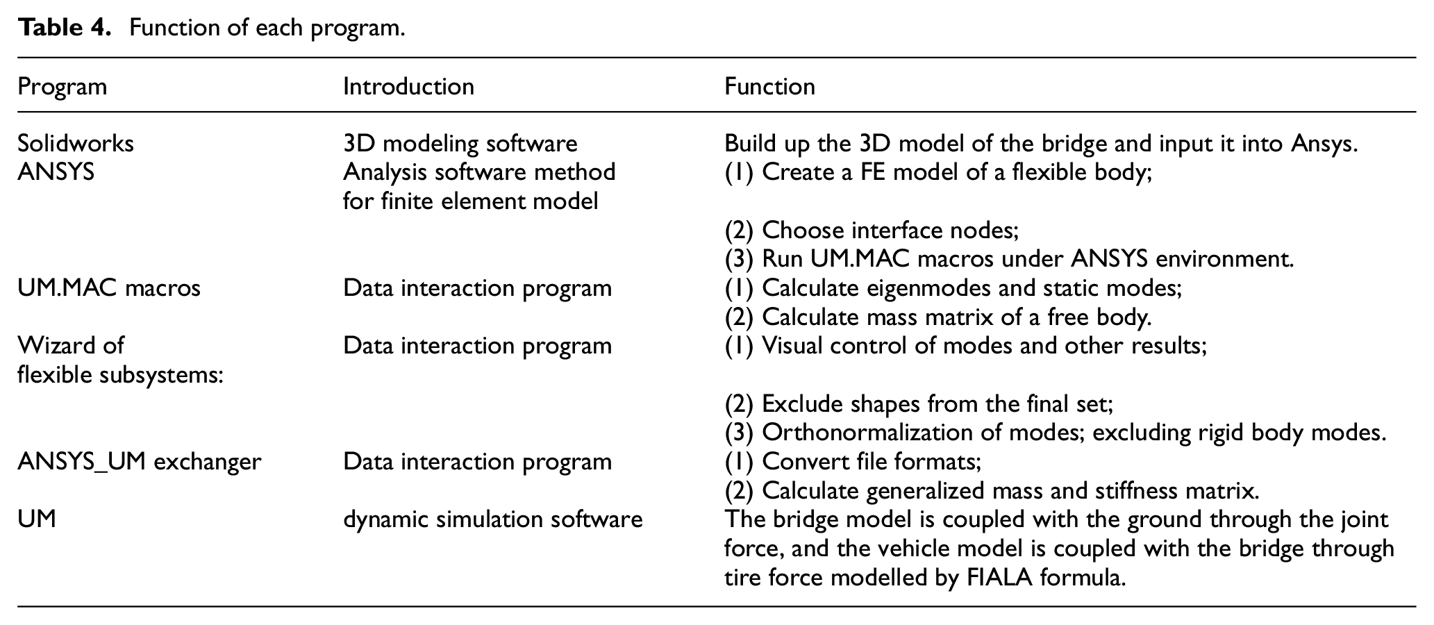
Nowadays, there are two methods for the dynamic simulations for vehicle system in the world, namely the multi rigid body dynamics and vehicle-bridge coupling dynamics. For the vehicle-bridge coupling dynamics, the 3D model of the Y shape bridge is built up in Solidworks. It contains the piers and the box girder with an open bottom. The piers and girder are connected by the pin shaft. The FE model is built up with the Shell 181 element in Ansys and inputted into UM. Six programs are needed in this process, ³⁰ shown in Table 4. In these software, Universal Mechanism (UM) is a new Russian dynamics simulation software for the multi body system. It can analyze not only rigid-body systems with multi-degrees of freedom, but also some complex rigid-flexible coupling systems. It is widely used in the machinery, automobiles, railway vehicles, aerospace, monorail, robots, and so on. ³¹

Table 4.

Function of each program.

Program	Introduction	Function
Solidworks	3D modeling software	Build up the 3D model of the bridge and input it into Ansys.
ANSYS	Analysis software method for finite element model	(1) Create a FE model of a flexible body;
		(2) Choose interface nodes;
		(3) Run UM.MAC macros under ANSYS environment.
UM.MAC macros	Data interaction program	(1) Calculate eigenmodes and static modes;
		(2) Calculate mass matrix of a free body.
Wizard of flexible subsystems:	Data interaction program	(1) Visual control of modes and other results;
		(2) Exclude shapes from the final set;
		(3) Orthonormalization of modes; excluding rigid body modes.
ANSYS_UM exchanger	Data interaction program	(1) Convert file formats;
		(2) Calculate generalized mass and stiffness matrix.
UM	dynamic simulation software	The bridge model is coupled with the ground through the joint force, and the vehicle model is coupled with the bridge through tire force modelled by FIALA formula.

Simulation process of the vehicle-bridge coupling dynamics

The linear multistep methods are chosen for simulation in the traditional researches. It is known in these researches that the historical derivatives will result in numerical instability. Park method, with no requirement of historical derivative information could be the solution. The multistep method $G_m$ , could be expressed as follows ³⁸ :

$$G_m=\sum _{i=0}^m({\alpha }_i{X}_{n-1-i}-\mathrm{\Delta }t{\beta }_i\frac{d{X}_{n-1-i}}{\mathrm{dt}})+T_m$$

(15)

Where, $T_m$ denotes the truncation error of the given method. ${\alpha }_i,{\beta }_i$ are the coefficients of the particular method.

The Park method could be defined as follows:

$$P_{m,n}=C_m{G}_m+C_n{G}_n$$

(16)

$C_m,C_n$ are constants.

Reference ³⁸ shows the comparison among the Houbolt method, trapezoidal method, and Park method. When the integration step is small, the result of trapezoidal rule is more accurate, but when the time step is larger, the result becomes unbounded.

Compared with Houbolt and Gear’s methods for the linear system, and Gear’s two-step and three-step methods and Houbolt method, Park method shows its great advantage over other integration methods.

Through all kinds of experiment, it is demonstrated that Park method is an implicit solver of the second order with a variable step size, for stiff ordinary differential equation and differential algebraic equation. Using this method, a more complex dynamic model could be solved.

The traditional modeling method for vehicle system are the multi rigid body dynamic method and vehicle-bridge coupling dynamic method.^31–36 The dynamic models of the two method are shown in Figure 7:

Figure 7.

Dynamic model: (a) multi-rigid body model, (b) vehicle-bridge coupling model.

The initial position of the vehicle and bridge will be calculated first. The tire force is calculated according to the dynamic response of the vehicle and bridge at the previous time point, then the dynamic response of the vehicle and bridge at the next time point will be obtained by the new tire forces. The detailed simulation process is shown in Figure 8.

Figure 8.

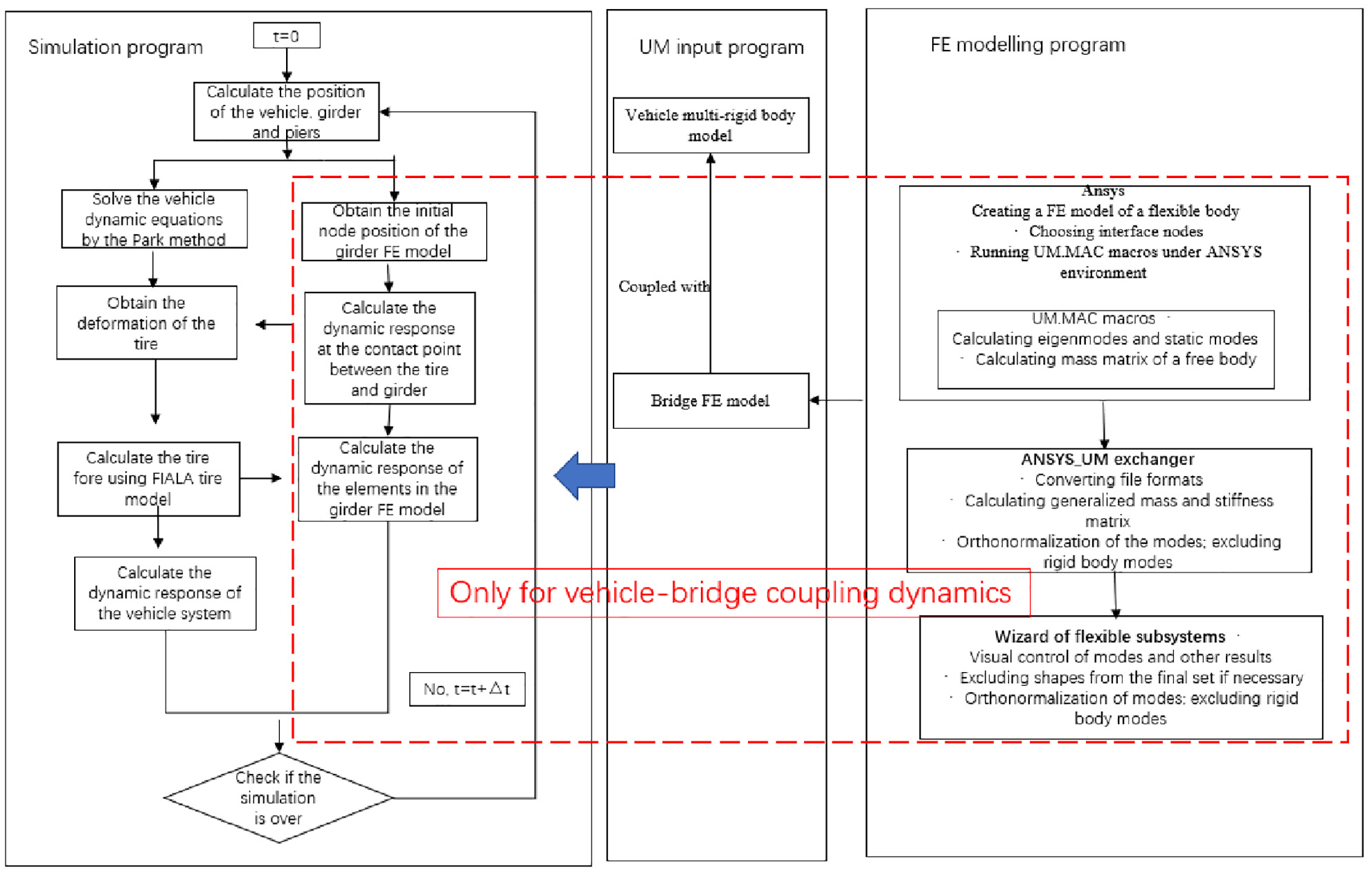
Flow chart of the integration of the vehicle-bridge coupling system.

Traditional parameter controlling strategy

There are two strategies to control the suspension parameters, which are called Matsim and Simat shown in Figure 9:

1. Matsim: The transferring function of is edited in a Simulink model as the control program. Input the control program into “dll” file which will be used as control element in dynamic software. When the simulation begins, the “dll” file will control the parameter which will be input into the dynamic system in the next period.

2. Simat: The dynamic model is linearized and input into Simulink as a matrix. In the Simulink integration space, it is shown as a system function module. When the simulation begins, the parameters are input into the system function. The transferring function will control the parameter which will be input into the dynamic system in the next period.

Figure 9.

Traditional parameter controlling strategy: (a) Matsim, (b) Simat.

Batch process for parameters

The major difference between the two strategies is the position of the integration space. Matsim uses the dynamics software as integration platform, but for Simat, the integration space is Simulink. However, both the two method are the real time control. That means, they both carry out one period for a vehicle to pass the bridge.

As for the batch process, it is needed to carry out a unique simulation for each group of parameters. The simplest method to achieve this goal is to use the Simulink as the integration space, and the control system is shown in Figure 10.

Figure 10.

Batch process using the Simulink as the integration space.

The practical experiment shows that the application of this method is limited. The integration solver in Simulink cannot solve the dynamic model which is complicated. Besides, the linearize process to transform the dynamic model into the system function can result in some errors in the result.

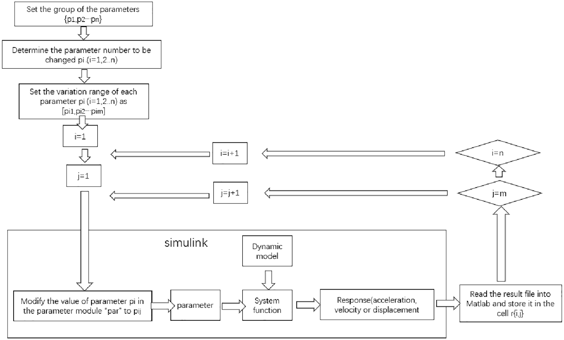
In order to enable the intelligent integration solved in the dynamic software, the batch process is as follows. Store the value ranges of each parameter in each vector in Matlab. For each simulation process, a numerical value will be selected from the vector and assigned to the corresponding parameter. Then, the parameter file “Par” in the UM software will be modified by the program. The DOS command to run the UM software will be automatically written in a “bat” file and run by Matlab. The simulation result file will be read and stored in a cell array in Matlab. Cyclic computation will be carried out till the end. This process is shown in Figure 11.

Figure 11.

Batch process using dynamic software as the integration space.

Result analysis

Comparison between the multi-rigid body dynamics and vehicle-bridge coupling dynamics

Sperling index, specified in GB5599 ³⁷ is an important index to evaluate the ride comfort of the railway trains. The lower the Sperling index is, the more stable the vehicle system is. In many countries like China, it is also applied in the study of the monorail. The following figure shows the comparison of the ride comfort response of the vehicle between the multi rigid body dynamics and vehicle bridge coupling dynamics. The vehicle speed is chosen as the decision variable input into the batch program. The result of Figure 12 shows the vibration of the bridge doesn’t cause a large error. So, in order to reduce the amount of calculation, the multi rigid body dynamics is carried out in the research of the effect of the vehicle parameters.

Figure 12.

Sperling index of the vehicle in difference vehicle speed: (a) lateral vibration (multi-rigid body dynamics), (b) lateral vibration (vehicle-bridge coupling dynamics), (c) vertical vibration (multi- rigid body dynamics), (d) vertical vibration (vehicle-bridge coupling dynamics).

The main components to alleviate the vibration are the lateral shock absorber, vertical shock absorber, air spring, anti-tilting shock absorber, guide wheel, stable wheel, driving wheel. This chapter will analyze the effect of these components on the vehicle. The research objectives are the lateral Sperling index, vertical Sperling index, maximum guide wheel force, maximum stable wheel force.

In the FIALA tire model, the radial damping of the wheel can be expressed as an equation for the radial stiffness, shown as follows.

$$D_z=2{\beta }_z\sqrt{m{C}_z}$$

(17)

${\beta }_z$ denotes the damping ratio of critical; m, the tire mass; $C_z$ , the tire radial stiffness.

When the radial stiffness of the wheel is determined, the radial damping of the wheel is also determined. Therefore, it is not necessary to analyze the effect of the wheel damping additionally.

Effect of all the parameters

The effects of the components on the lateral Sperling index are shown in Figures 13–15. When the lateral stiffness of the air spring ranges from 0.1 to 0.4 MN/m, the lateral Sperling index increases from 1.85 to 2. When the radial stiffness of the driving wheel increase from 0.2 to 2 MN/m, the lateral Sperling index increases from 1.6 to 2.1. When the radial stiffness of the guide wheel increase from 0.2 to 2 MN/m, the lateral Sperling index increases from 1.7 to 1.9. As shown in the figures, reducing the lateral stiffness of the air spring and the radial stiffness of the guide wheel and driving wheel can significantly alleviate the lateral vibration. The damping of the lateral shock absorber, plays a greater role than the lateral damping of the air spring. As known in the FIALA formula, the tire side force varies with the radial force. It is just like that there is a lateral spring element between the vehicle and the rail surface, whose stiffness is proportional to the radial stiffness of the driving wheel. So, it is not difficult to explain why the stiffness of driving wheels has such a great effect on the lateral vibration of the vehicle.

Figure 13.

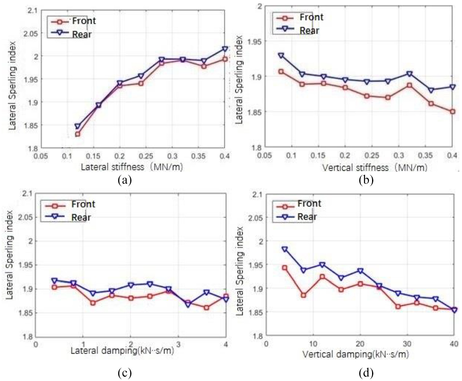
Effect of the air spring parameter on the lateral Sperling index: (a) lateral stiffness; (b) vertical stiffness; (c) lateral damping; and (d) vertical damping.

Figure 14.

Effect of the damping of the shock absorber on the lateral Sperling index: (a) lateral shock absorber; (b) vertical shock absorber; and (c) anti-tilting shock absorber.

Figure 15.

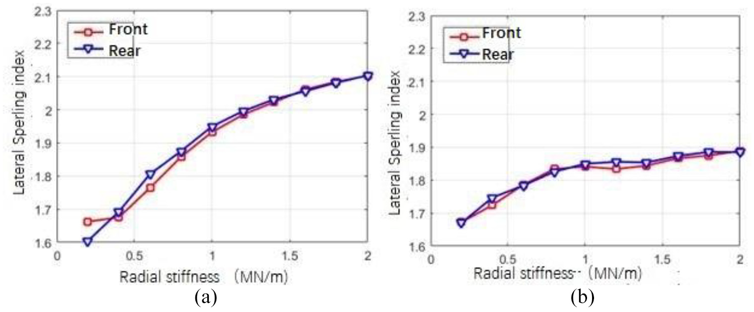
Effect of the wheel radial stiffness on the lateral Sperling index: (a) driving wheel and (b) guide wheel.

The effect of the parameters on the vertical Sperling index of the vehicle is shown in Figures 16–18. When the vertical stiffness of the air spring varies from 0.08 to 0.4 MN/m, the vertical Sperling index of the vehicle front position varies from 2.3 to 2.4, the vertical Sperling index of the vehicle rear position varies from 2.2 to 2.3. When the vertical damping of the air spring varies from 4 to 40 kN·s/m, the vertical Sperling index of the vehicle front position increases from 2.2 to 2.4, the vertical Sperling index of the vehicle rear position increases from 2.1 to 2.3. When the radial stiffness of the driving wheel varies from 0.2 to 2 MN/m, the vertical Sperling index of the vehicle increases from 2 to 2.6. As you can see, the vertical stiffness and damping of the air spring, radial stiffness of the driving wheel play an important role on the alleviation of the vertical vibrations. Compared to the stiffness, the damping of the air spring shows greater importance. Due to the small damping, the vertical shock absorber doesn’t seem to be able to reduce the vibration. As a result, it should be removed or replaced by another absorber with a larger damping.

Figure 16.

Effect of the air spring parameter on the vertical Sperling index: (a) lateral stiffness; (b) vertical stiffness; (c) lateral damping; and (d) vertical damping.

Figure 17.

Effect of the damping of the shock absorber on the vertical Sperling index: (a) lateral shock absorber; (b) vertical shock absorber; and (c) anti-tilting shock absorber.

Figure 18.

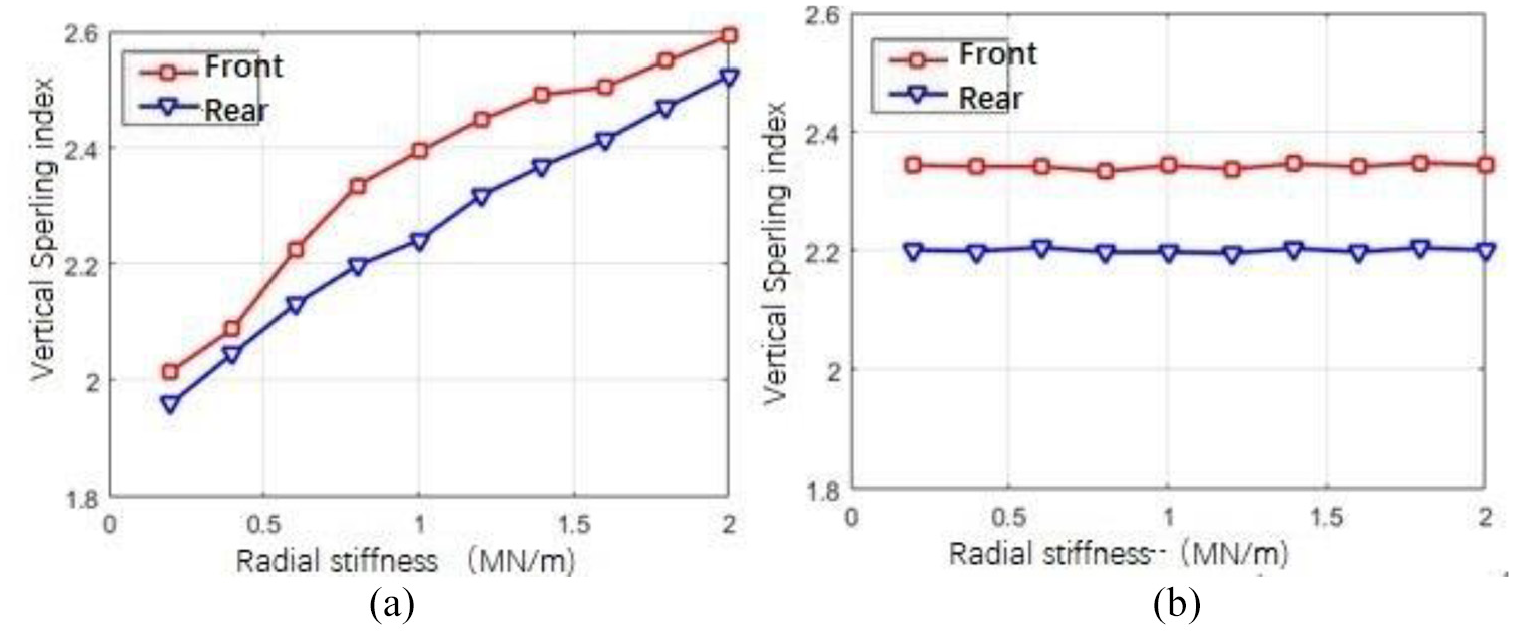
Effect of the wheel radial stiffness on the vertical Sperling index: (a) driving wheel and (b) guide wheel.

Shown in the Figures 19–21, when the radial stiffness of the driving wheel varies from 0.2 to 2 MN/m, the radial force of the guide wheel increases from 1 to 5 kN. The parameter which affect the guide wheel force greatest is the radial stiffness of the driving wheel. Other parameters including that for the lateral vibration alleviation show little effect on the radial force of the guide wheel.

Figure 19.

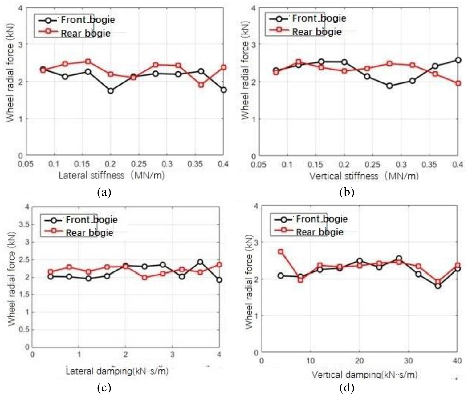
Effect of the air spring parameter on guide wheel force: (a) lateral stiffness; (b) vertical stiffness; (c) lateral damping; and (d) vertical damping.

Figure 20.

Effect of the damping of the shock absorber on guide wheel force: (a) lateral shock absorber; (b) vertical shock absorber; and (c) anti-tilting shock absorber.

Figure 21.

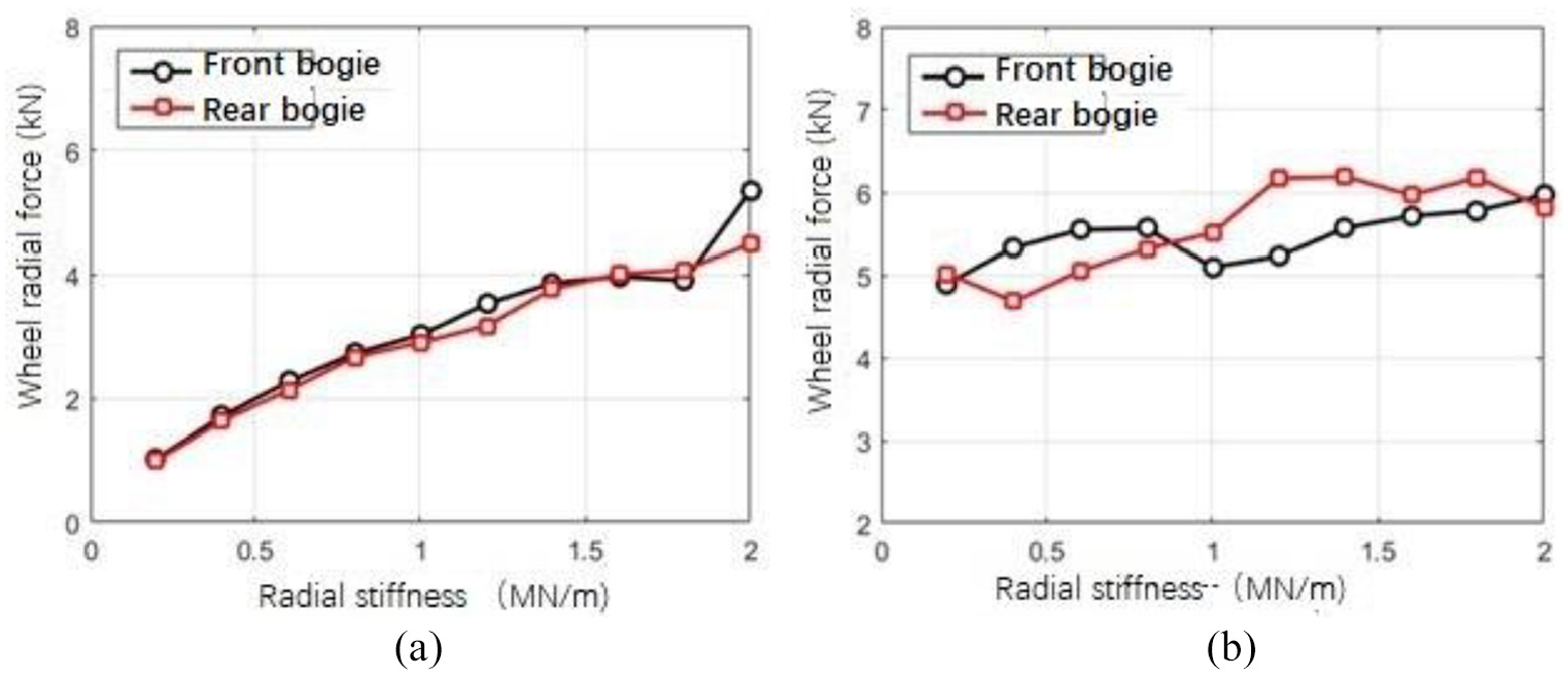
Effect of the wheel radial stiffness on guide wheel force: (a) driving wheel and (b) guide wheel.

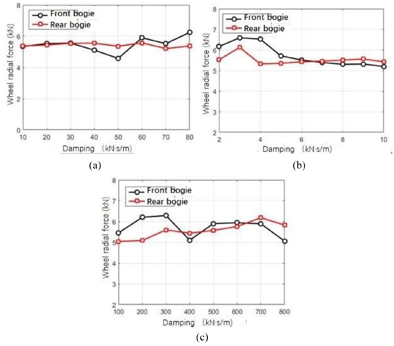
As you can see in the results of Figures 22–24, when the radial stiffness of the driving wheel varies from 0.2 to 2 MN/m, the radial force of the stable wheel increases from 1 to 3 kN. When the radial stiffness of the guide wheel varies from 0.2 to 2 MN/m, the radial force of the stable wheel increases from 1 to 3 kN. Except for the guide wheel stiffness, the radial stiffness of the driving wheel also plays an important role. Large stiffness of the driving wheel is not helpful to reduce the difference of the forces between left and right driving wheels caused by the road irregularities, result in the fierce rolling movement of the bogie. This rolling movement can only be alleviated by the stable wheel which provides a moment to prevent the bogie overturning. As a result, the stable wheel force will increase.

Figure 22.

Effect of the air spring parameter on stable wheel force: (a) lateral stiffness; (b) vertical stiffness; (c) lateral damping; and (d) vertical damping.

Figure 23.

Effect of the damping of the shock absorber on stable wheel force: (a) lateral shock absorber; (b) vertical shock absorber; and (c) anti-tilting shock absorber.

Figure 24.

Effect of the wheel radial stiffness on stable wheel force: (a) driving wheel and (b) guide wheel.

Conclusion

With various of intelligent solvers like “Park” solver and tire models like “FIALA model, the UM software seems the best choice to analyze the dynamic properties of the monorail. The complicated model which cannot be solved through the traditional method could be solved in this software. The vehicle-bridge coupling dynamics, which contains the complicated FE model of the bridge, will take a lot of time during the simulation. The parameters cannot be changed during the simulation. In order to analyze the effect of each parameter on the vehicle, an intelligent co-simulation method is introduced. This process enables the simulation to run in the UM software, and the advantages of the algorithm will be remained. Cyclic computation will be carried out till the end. Then, the effect of the parameters on the system could be analyzed in the study.

Known from the research, when the lateral stiffness of the air spring ranges from 0.1 to 0.4 MN/m, the lateral Sperling index increases from 1.85 to 2. When the radial stiffness of the driving wheel increase from 0.2 to 2 MN/m, the lateral Sperling index increases from 1.6 to 2.1. When the radial stiffness of the guide wheel increase from 0.2 to 2 MN/m, the lateral Sperling index increases from 1.7 to 1.9. When the vertical stiffness of the air spring varies from 0.08 to 0.4 MN/m, the vertical Sperling index of the vehicle front position varies from 2.3 to 2.4, the vertical Sperling index of the vehicle rear position varies from 2.2 to 2.3. When the vertical damping of the air spring varies from 4 to 40 kN·s/m, the vertical Sperling index of the vehicle front position increases from 2.2 to 2.4, the vertical Sperling index of the vehicle rear position increases from 2.1 to 2.3. When the radial stiffness of the driving wheel varies from 0.2 to 2 MN/m, the vertical Sperling index of the vehicle increases from 2 to 2.6. When the radial stiffness of the driving wheel varies from 0.2 to 2 MN/m, the radial force of the guide wheel increases from 1 to 5 kN. When the radial stiffness of the driving wheel varies from 0.2 to 2 MN/m, the radial force of the stable wheel increases from 1 to 3 kN. When the radial stiffness of the guide wheel varies from 0.2 to 2 MN/m, the radial force of the stable wheel increases from 1 to 3 kN. Reducing the lateral stiffness of the air spring and the radial stiffness of the guide wheel can significantly alleviate the lateral vibration. The damping of the lateral shock absorber, plays a greater role than the lateral damping of the air spring. The lateral vibration can also be alleviated by reducing the radial stiffness of the driving wheel. The vertical stiffness and damping of the air spring, radial stiffness of the driving wheel plays an important role on the alleviation of the vertical vibrations. Compared to the stiffness, the damping of the air spring shows greater importance. Due to the small damping, the vertical shock absorber doesn’t seem to be able to alleviate the vibration. As a result, it should be removed or replaced by another absorber with a larger damping. The parameter which affect the guide wheel force greatest is the radial stiffness of the guide wheel. Other parameters including that for the lateral vibration alleviation show little effect on the radial force of the guide wheel. Except for the guide wheel stiffness, the radial stiffness of the driving wheel also plays an important role to control the stable wheel force.

Supplemental Material

Appendix – Supplemental material for Intelligent batch process method for analyzing the effect of the suspension parameters on the vibration of the suspended monorail

Supplemental material, Appendix for Intelligent batch process method for analyzing the effect of the suspension parameters on the vibration of the suspended monorail by Yongzhi Jiang, Pingbo Wu, Jing Zeng, Xingwen Wu, Xing Wang and Qinglie He in Advances in Mechanical Engineering