Sage Journals: Discover world-class research

Abstract

A model-driven fault diagnosis method for slant cracks in aero-hydraulic straight pipes is presented in this paper. First, fracture mechanics theory and the principle of strain energy release are used to derive an expression for the local flexibility coefficient of straight pipes with slant cracks. The inverse method of total flexibility is used to calculate the stiffness matrix of straight pipe elements with slant cracks. Second, the Euler-Bernoulli beam model theory is used in conjunction with the finite element method to construct a dynamic model of the cracked pipe. Finally, a contour map method is used to diagnose the slant crack fault and quantitatively determine the crack position and depth. Experimental results show that the proposed method can accurately and effectively identify a slant crack fault in aero-hydraulic pipelines.

Keywords

Fault diagnosis aero-hydraulic straight pipe slant crack stress intensity factor finite element method

Introduction

Hydraulic pipes have a wide range of applications in the aerospace field. At present, the development of high-pressure, lightweight, and intelligent applications of aero-equipment require hydraulic pipes to operate under severe fluid pulsation over extended periods. Cumulative damage occurs under high vibrational stress induced by structural resonance in the pipeline, and multiple cycles lead to crack propagation and fracture.^1,2 The vibrations caused by pipeline cracks have strong non-linearity and non-stationarity, such the resulting damage is considerably more severe than that from general faults.^3,4 Therefore, research on vibration failure and crack fault diagnosis of aero-hydraulic pipelines is extremely significant for prolonging the service life of aero-engine hydraulic pipeline systems.

Some success has been achieved in previous research studies on the model-based dynamic characteristics of hydraulic pipelines. These studies have focused on constructing pipeline models and determining the pipeline fluid-solid coupling vibration mechanism.^5,6 Current pipeline models include beam models and shell models. The beam model is applicable when the length of the pipeline is much larger than the cross-sectional diameter. The shell model is more reasonable when the pipeline length is small relative to the diameter of the cross-section. Pei-xin Gao et al.^7–9 proposed a model reduction method for complex aeronautical hydraulic pipeline systems and studied the vibration response of hydraulic pipeline systems under multi-source excitations. Zhai Hong-bo and Xiaoping Ouyang et al.^10,11 analysed the vibration response and modal characteristics of hydraulic pipelines.

Hydraulic pipelines account for the largest proportion of all pipelines. These pipelines are easily damaged during service because of fatigue, overload, collision and other reasons. Statistics show that the failure of aeronautical hydraulic pipelines accounts for more than 50% of accidents in aircraft systems. Timely detection of hydraulic pipeline failure is required to prevent serious safety accidents.^12,13 In general, a crack in an actual environment propagates at an angle (that is not always 90°) to the longitudinal direction. In modelling cracked pipelines, the change in the pipeline stiffness caused by cracks is first determined. Then, the effect of this change in the stiffness on the inherent characteristics of the pipeline is studied. Yongfeng Yang et al.¹⁴ analysed the dynamic characteristics of a hollow shaft considering uncertainties in the parameters of a crack model. Fusheng Wang et al.¹⁵ applied the finite element model to study the factors affecting crack propagation in a hydraulic pipeline. Ridong Bao et al.^16,17 studied the dynamic characteristics of cracked pipelines with general and elastic support at both ends.

Scholars have used frequency data to identify crack faults.^18–20 When a crack occurs in a structure, the material physical parameters change and affect the inherent characteristics of the structure. Therefore, the change in the natural frequency can be used to monitor crack damage. Fault diagnosis of structural cracks can be performed by correlating the natural frequency with the structural damage. The change law of the natural frequency reflects the degree of structural damage.

Most current research studies have considered solid beam structures and mainly straight cracks. Therefore, a model-driven fault diagnosis method for a slant crack in aero-hydraulic straight pipes is proposed in this paper. The local flexibility coefficient and the element matrix of the cracked pipeline are calculated and used to construct a finite element model. Measured natural frequencies are as input as parameters to the proposed model to identify slant crack faults on hydraulic pipelines and quantify the crack location and depth.

Establishment of finite element model

The Euler-Bernoulli beam model theory is used to construct a finite element model of a straight pipe with a slant crack. The hydraulic straight pipe element is shown in Figure 1, where the element nodes in the local coordinate system are denoted by i and j. Consider that each node has three degrees of freedom (the transverse and longitudinal displacements of the node and the angular displacement of the node cross-section) for an element length l_e. The displacement vector of the pipeline element node is²¹

{D^{e}} = {[u_{i}, θ_{i}, v_{i}, u_{j}, θ_{j}, v_{j}]}^{T}

(1)

Figure 1.

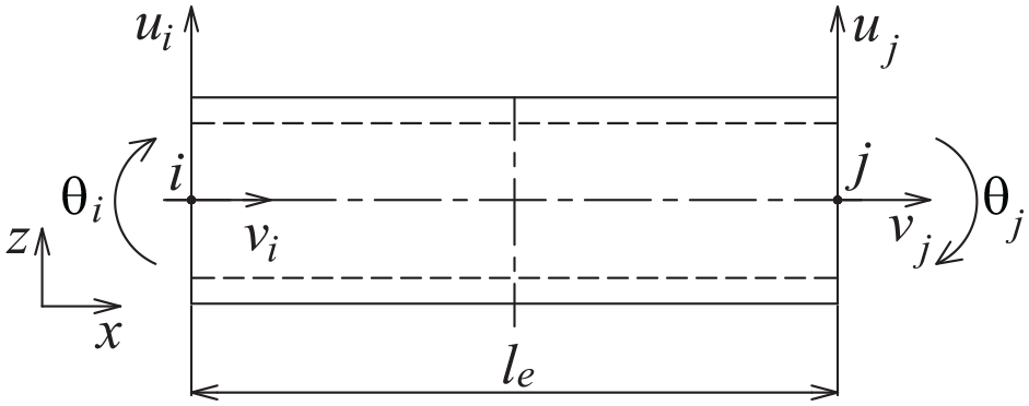
Hydraulic straight pipe element.

The stiffness matrix for the elements of the hydraulic straight pipe is

K_{g} = [\begin{matrix} \frac{EA}{l_{e}} & 0 & 0 & - \frac{EA}{l_{e}} & 0 & 0 \\ 0 & \frac{12 EI}{l_{e}^{3}} & \frac{6 EI}{l_{e}^{2}} & 0 & - \frac{12 EI}{l_{e}^{3}} & \frac{6 EI}{l_{e}^{2}} \\ 0 & \frac{6 EI}{l_{e}^{2}} & \frac{4 EI}{l_{e}} & 0 & - \frac{6 EI}{l_{e}^{2}} & \frac{2 EI}{l_{e}} \\ - \frac{EA}{l_{e}} & 0 & 0 & \frac{EA}{l_{e}} & 0 & 0 \\ 0 & - \frac{12 EI}{l_{e}^{3}} & - \frac{6 EI}{l_{e}^{2}} & 0 & \frac{12 EI}{l_{e}^{3}} & - \frac{6 EI}{l_{e}^{2}} \\ 0 & \frac{6 EI}{l_{e}^{2}} & \frac{2 EI}{l_{e}} & 0 & - \frac{6 EI}{l_{e}^{2}} & \frac{4 EI}{l_{e}} \end{matrix}]

(2)

The mass matrix for the elements of the hydraulic straight pipe is

\begin{matrix} M_{g} = \\ [\begin{matrix} \frac{ρ A l_{e}}{3} & 0 & 0 & - \frac{ρ A l_{e}}{6} & 0 & 0 \\ 0 & \frac{13 ρ A l_{e}}{35} & \frac{11 ρ {Al}_{e}^{2}}{210} & 0 & \frac{9 ρ A l_{e}}{70} & - \frac{13 ρ A l_{e}}{420} \\ 0 & \frac{11 ρ {Al}_{e}^{2}}{210} & \frac{ρ {Al}_{e}^{3}}{105} & 0 & \frac{13 ρ A l_{e}}{420} & - \frac{ρ {Al}_{e}^{3}}{140} \\ - \frac{ρ A l_{e}}{6} & 0 & 0 & \frac{ρ A l_{e}}{3} & 0 & 0 \\ 0 & \frac{9 ρ A l_{e}}{70} & \frac{13 ρ A l_{e}}{420} & 0 & \frac{13 ρ A l_{e}}{35} & - \frac{11 ρ {Al}_{e}^{2}}{210} \\ 0 & - \frac{13 ρ A l_{e}}{420} & - \frac{ρ {Al}_{e}^{3}}{140} & 0 & - \frac{11 ρ {Al}_{e}^{2}}{210} & \frac{ρ {Al}_{e}^{3}}{105} \end{matrix}] \end{matrix}

(3)

where E is the elastic modulus of the pipeline material, I is the moment of inertia of the pipeline section, A is the cross-sectional area of the pipeline, ρ is the pipe density, and x is the coordinate along the longitudinal direction of the pipeline element.

An aero-engine hydraulic piping system is an extremely complex structure. Multiple field coupling factors affect the hydraulic piping during operation.²² An aero-hydraulic straight pipe is usually fixed on the body of the structure, and mechanical and fluid coupling vibrations are generated under the combined action of basic and pump source excitations. Figure 2 is a schematic of a hydraulic straight pipe with fixed ends in slant crack failure. The pipeline is divided into 20 elements, and the slant crack failure is located at the 11th element.

Figure 2.

Structural diagram of slant crack in a hydraulic straight pipe

A slant crack fault changes the local flexibility of the pipeline structure. The local flexibility coefficient must be determined to calculate the stiffness matrix of the elements of a straight pipe with a slant crack and is therefore key in constructing a corresponding finite element model. We follow the procedure developed by Dimarogonas²³ to determine the local flexibility of a cracked rotating shaft. The hydraulic pipeline is divided into a series of thin plates of thickness dβ. In-plane cracked beam theory is used to determine the additional strain energy of each thin plate, and numerical integration is used to obtain the local flexibility coefficient of the straight pipe element with slant cracks. A straight pipe element with a slant crack is shown in Figure 3. The pipeline element is subject to the combined action of the axial force P₁, the shear force P₂ and the bending moment P₃. The direction of the force is symmetrical about the central axis of the pipeline element.

Figure 3.

Straight pipeline element with slant crack.

The top view of the hydraulic straight pipe element with a slant crack is shown in Figure 4. The angle between the crack edge and the pipeline axis is denoted by θ (hereinafter referred to as the crack angle, which is 90° for a straight crack), β is the distance between the thin plate and the Z-axis, and l_c is the crack position. The crack size is the distance between the crack midline and the left end face of the straight pipe element.

Figure 4.

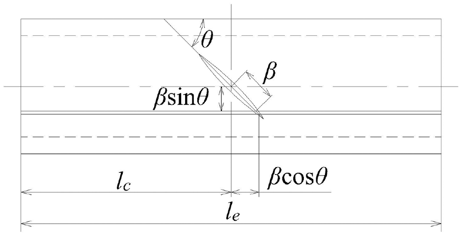
Top view of straight pipe element with slant crack.

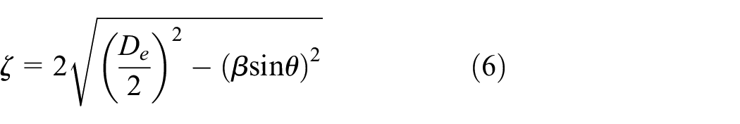
A cross-sectional view along the crack edge of the hydraulic straight pipe element with a diagonal crack is shown in Figure 5: a is the crack depth; D_e and D_i are the outer and inner pipe diameters respectively; b is the crack half-width at the cross-section; and α and ζ are the local depth variable and the height of the rectangular integral strip, respectively.

Figure 5.

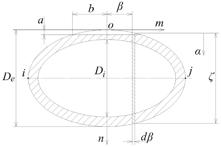
Sectional view of hydraulic diagonal crack straight pipe element along crack edge.

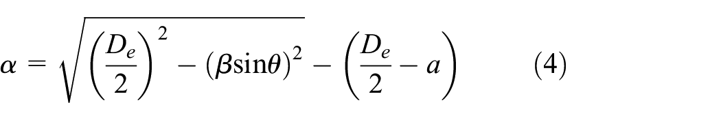
The geometric relationships in Figures 4 and 5 are used to obtain the following expressions:

α = \sqrt{{(\frac{D_{e}}{2})}^{2} - {(β \sin θ)}^{2}} - (\frac{D_{e}}{2} - a)

(4)

b = \frac{\sqrt{{(\frac{D_{e}}{2})}^{2} - {(\frac{D_{e}}{2} - a)}^{2}}}{\sin θ}

(5)

ζ = 2 \sqrt{{(\frac{D_{e}}{2})}^{2} - {(β \sin θ)}^{2}}

(6)

The stress intensity factor of the crack region of each rectangular integral strip for a slant crack in a hydraulic straight pipe under the combined action of the axial force, the shear force and the bending moment is

K_{I}^{1} = \frac{4 P_{1}}{π D_{e}^{2} (1 - γ^{2})} si n^{2} θ \sqrt{π α} F_{1} (\frac{α}{ζ})

(7)

K_{I}^{2} = \frac{32 P_{2} (l_{c} + β \cos θ) ζ}{π D_{e}^{4} (1 - γ^{4})} si n^{2} θ \sqrt{π α} F_{2} (\frac{α}{ζ})

(8)

K_{I}^{3} = \frac{32 P_{3} ζ}{π D_{e}^{4} (1 - γ^{4})} si n^{2} θ \sqrt{π α} F_{2} (\frac{α}{ζ})

(9)

K_{II}^{2} = \frac{4 k P_{2}}{π D_{e}^{2} (1 - γ^{2})} \sin θ \sqrt{π α} F_{II} (\frac{α}{ζ})

(10)

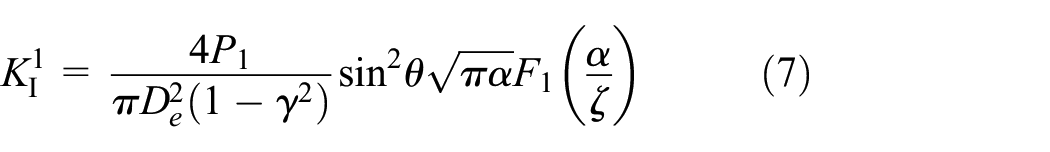
where k is the shear coefficient.²⁴ For a circular section, $k = \frac{6 (1 + ν) {(1 + γ^{2})}^{2}}{(7 + 6 ν) {(1 + γ^{2})}^{2} + (20 + 12 ν) γ^{2}}$ , where γ = D_i /D_e; and ν is Poisson’s ratio. The stress intensity factor is used to derive the local flexibility coefficient of a straight pipe with slant cracks.

According to the basic theory of local flexibility, the release rate of additional strain energy caused by slant cracks is

J = \frac{1}{E'} [{(K_{I}^{1} + K_{I}^{2} + K_{I}^{3})}^{2} + {(K_{II}^{2})}^{2}]

(11)

where E′ is Young’s elastic modulus, and E′=E/(1-ν²) for the plane strain state, and E′=E for the plane stress state.

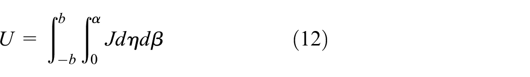
According to fracture mechanics theory, the additional strain energy resulting from the slant crack in the hydraulic straight pipe is

U = \int_{- b}^{b} \int_{0}^{α} Jd η d β

(12)

Then, the local flexibility coefficient for the cracked pipe is expressed as

c_{ij} = \frac{\partial^{2} U}{\partial P_{i} \partial P_{j}} = \frac{\partial^{2}}{\partial P_{i} \partial P_{j}} \int_{- b}^{b} \int_{0}^{α} Jd η d β (i, j = 1, 2, 3)

(13)

Considering the influence of the shear force and the shear coefficient, the local flexibility coefficient of a straight pipe with slant cracks is

c_{11} = \frac{32}{E' π D_{e}^{4} {(1 - γ^{2})}^{2}} si n^{4} θ \int_{- b}^{b} \int_{0}^{α} F_{1}^{2} (η / ζ) η d η d β

(14)

\begin{matrix} c_{12} = \frac{256}{E' π D_{e}^{6} (1 - γ^{2}) (1 - γ^{4})} si n^{4} θ \\ \int_{- b}^{b} \int_{0}^{α} l_{s} ζ F_{1} (η / ζ) F_{2} (η / ζ) η d η d β \end{matrix}

(15)

\begin{matrix} c_{13} = \frac{256}{E' π D_{e}^{6} (1 - γ^{2}) (1 - γ^{4})} \\ si n^{4} θ \int_{- b}^{b} \int_{0}^{α} ζ F_{1} (η / ζ) F_{2} (η / ζ) η d η d β \end{matrix}

(16)

\begin{matrix} c_{22} = \frac{2048}{E' π D_{e}^{8} {(1 - γ^{4})}^{2}} si n^{4} θ \int_{- b}^{b} \int_{0}^{α} l_{s}^{2} ζ^{2} F_{2}^{2} (η / ζ) η d η d β \\ + \frac{32 k^{2}}{E' π D_{e}^{4} {(1 - γ^{2})}^{2}} si n^{2} θ \int_{- b}^{b} \int_{0}^{α} F_{II}^{2} (η / ζ) η d η d β \end{matrix}

(17)

c_{23} = \frac{2048}{E' π D_{e}^{8} {(1 - γ^{4})}^{2}} si n^{4} θ \int_{- b}^{b} \int_{0}^{α} l_{s} ζ^{2} F_{2}^{2} (η / ζ) η d η d β

(18)

c_{33} = \frac{2048}{E' π D_{e}^{8} {(1 - γ^{4})}^{2}} si n^{4} θ \int_{- b}^{b} \int_{0}^{α} ζ^{2} F_{2}^{2} (η / ζ) η d η d β

(19)

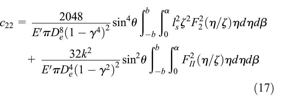
where l_s=l_c+βcosθ, and F₁(s), F₂(s) and F_II(s) are correction factors for the stress intensity factor of the pipeline crack:

\begin{matrix} F_{1} (s) = \sqrt{\tan λ / λ} \times \\ (0.751 + 2.02 s + 0.37 {(1 - \sin λ)}^{3}) / \cos λ \end{matrix}

(20)

F_{2} (s) = \sqrt{\tan λ / λ} \times (0.923 + 0.199 {(1 - \sin λ)}^{4}) / \cos λ

(21)

F_{II} (s) = (1.122 - 0.561 s + 0.085 s^{2} + 0.18 s^{3}) / \sqrt{1 - s}

(22)

where $s = \frac{η}{ζ}$ and $λ = \frac{π}{2} \times s$ .

The local flexibility for the cracked pipe is then given by

C_{crack} = [\begin{matrix} c_{11} & - c_{12} & - c_{13} \\ - c_{21} & c_{22} & c_{23} \\ - c_{31} & c_{32} & c_{33} \end{matrix}]

(23)

Using the total flexibility inversion method,²⁵ the total flexibility of a straight pipe with a slant crack is equal to the sum of the element flexibility without cracks and the flexibility in the presence of cracks, that is,

\begin{matrix} C_{sum} = C_{int act} + C_{crack} \\ = [\begin{matrix} \frac{l_{e}}{EA} + c_{11} & - c_{12} & - c_{13} \\ - c_{21} & \frac{l_{e}^{3}}{3 EI} + c_{22} & \frac{l_{e}^{2}}{2 EI} + c_{23} \\ - c_{31} & \frac{l_{e}^{2}}{2 EI} + c_{32} & \frac{l_{e}}{EI} + c_{33} \end{matrix}] \end{matrix}

(24)

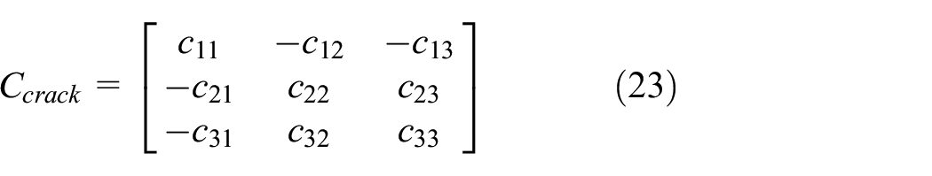
The stiffness matrix of a straight pipe element with a slant crack is

K_{g}^{c} = {Tc}_{sum}^{- 1} T^{T}

(25)

where $T = {[\begin{matrix} - 1 & 0 & 0 & 1 & 0 & 0 \\ 0 & - 1 & - l_{e} & 0 & 1 & 0 \\ 0 & 0 & - 1 & 0 & 0 & 1 \end{matrix}]}^{T}$ is the transformation matrix.

For a relatively small crack, the pipeline quality can be considered to be unchanged by the occurrence of the crack. The uniform element mass matrix of the pipeline system is M_g. The stiffness matrix of the pipeline elements with and without diagonal cracks are K_g^c and K_g, respectively. The stiffness and mass matrix of the elements of the hydraulic straight pipe are grouped into an overall matrix. Finally, the frequency equation of the hydraulic straight pipe system can be written as

| K - ω_{i}^{2} M | ϕ = 0

(26)

where M is the mass matrix, K is the stiffness matrix, and ω_i (i=1,2,…) is the natural frequency of the system. The frequency equation is solved to yield the natural frequencies of each order of the pipeline system.

Numerical calculation and experimental verification

Calculation of local flexibility coefficient of hydraulic straight pipe with slant crack

A correct solution for the local flexibility coefficient of a straight pipe with a slant crack is a prerequisite for constructing a corresponding finite element model. In this study, the effect of breathing cracks is not considered, and the two ends of the pipeline have fixed support. Numerical integration is used to calculate the local flexibility coefficient of the pipeline. Experiments are carried out on an aero-stainless-steel hydraulic straight pipe. The parameters of the pipeline are shown in Table 1.

Table 1.

Material parameters and geometric dimensions of hydraulic straight pipe.

Parameter	Value
Elastic modulus E	1.93×10¹¹ Pa
Poisson’s ratio μ	0.3
Density ρ	7930 kg/m³
Length L	540 mm
Outer diameter D_e	16 mm
Inner diameter D_i	12 mm

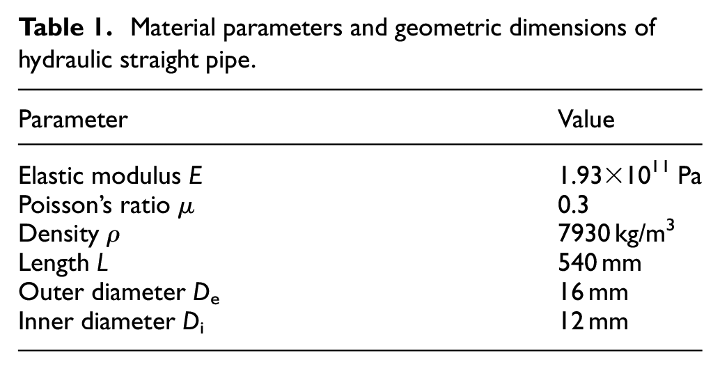
Specifications of hydraulic straight pipe: γ = D_i/D_e= 0.75

First, the crack position is fixed at l_c = 7.2D_e, and the crack angle is set to 30°, 45°, 60° and 90° (straight cracks). The local flexibility coefficient is calculated for different crack depths using equations (14) to (19). Then, the crack angle is fixed at 45°, and the local flexibility coefficient is calculated for different crack positions and depths. The results are shown in Figures 6 and 7.

Figure 6.

Variation in local flexibility coefficient with crack angle.

Figure 7.

Variation in local flexibility coefficient with crack location.

Figure 6 shows that (1) the local flexibility coefficients c (i, j) for different crack angles gradually increase with the crack depth for a fixed slant crack location, and (2) the local flexibility coefficients increase with the crack angle for a fixed slant crack location and depth.

Figure 7 shows that for a fixed crack angle, (1) the local flexibility coefficients c (i, j) at different crack locations gradually increase with the crack depth, and (2) the local flexibility coefficient is higher the farther the crack is from the fixed end for a constant crack depth. This result is obtained because as the crack distance increases, the bending moment introduced by the shear force P₂ also increases, thereby increasing the local flexibility coefficient.

Modal experiment verification

A slant crack failure is artificially implanted on the outer wall of a hydraulic straight pipe that is fixed on a table. A force hammer is used as the pulse excitation source, and an acceleration sensor and an LMS data acquisition system are used to measure the inherent characteristics of the slant cracks at different locations, depths and angles in the straight pipe. Figure 8 shows the uncracked and failed hydraulic straight pipe, and Figure 9 shows the modal test.

Figure 8.

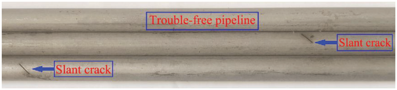
Slant crack failure in hydraulic straight pipe.

Figure 9.

Modal test of slant crack failure (a) at end and (b) in the middle of hydraulic straight pipe.

We correct the elastic modulus for the measured natural frequency of the uncracked hydraulic straight pipe.^26,27 The modified elastic modulus is then used to calculate the inherent characteristics of the straight pipe to reduce the frequency error between the theoretical calculation and the experimental measurement. The measured natural frequency of the uncracked hydraulic straight pipe is used as an input parameter with the following characteristic equation:

| ω_{i}^{2} M - \frac{E_{c}}{E} K | = 0

(27)

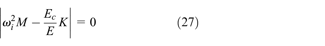
where M is the overall mass; K is the stiffness matrix; and E_c is the modified elastic modulus obtained by solving the frequency equation. In this paper, the first and second natural frequencies of the uncracked pipe are experimentally measured to be 280.00 Hz and 1506.30 Hz, respectively. The impulse response signal and frequency response of the uncracked pipe are shown in Figure 10. Using equation (27), E_c of the hydraulic straight pipe is calculated to be 166.77 GPa.

Figure 10.

(a) Impulse response signal and (b) frequency response of uncracked hydraulic straight pipe.

Equations (14) to (19) show that changes in parameters, such as the crack location, depth and included angle, affect the local flexibility of the pipeline structure, which in turn changes the natural frequency. This change in the natural frequency of the structure is more distinct in a thin-walled pipeline. To ensure the accuracy of the data, each pipeline is measured six times during the test and the results are averaged to obtain the test measurement. Before each measurement, the system is checked to determine whether the boundary conditions have been loosened by the action of the force hammer. Seven crack conditions are investigated in the experimental tests. The test results obtained under condition 1 are shown in Figure 11. The numerical and experimental results for the first and second natural frequencies of the hydraulic straight pipe are compared in Tables 2 and 3, respectively, using the relative error calculation formula below:

\frac{| E_{i} - F_{i} |}{E_{i}} \times 100 %

(28)

Figure 11.

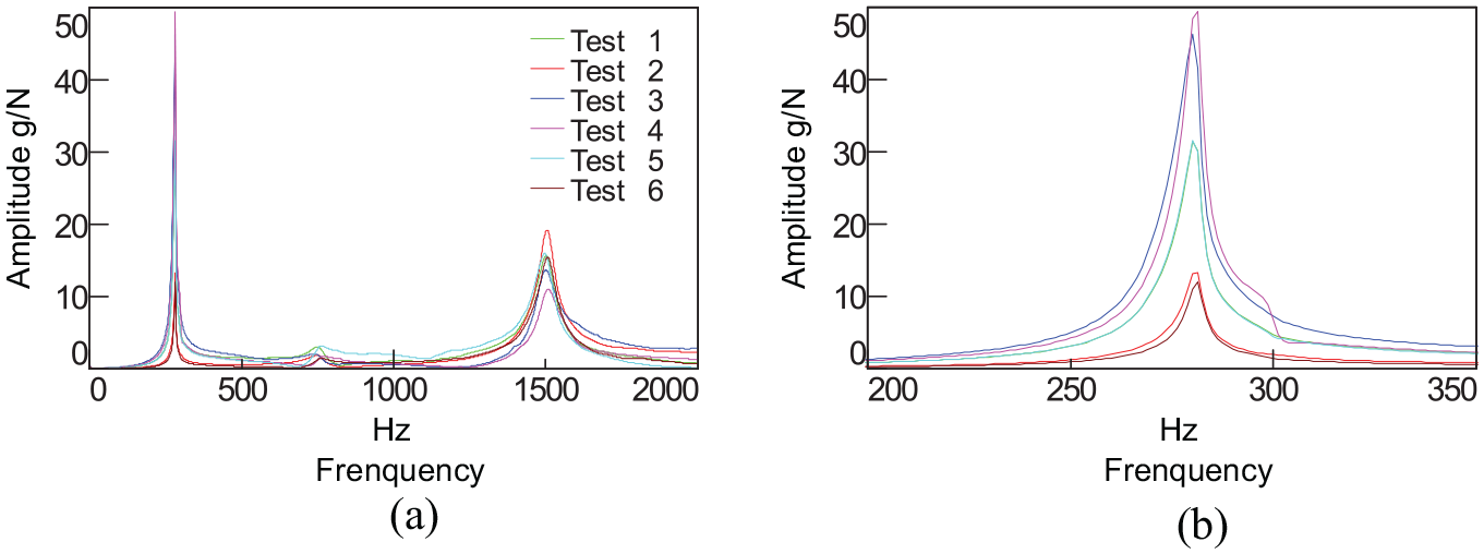
(a) Frequency response function for case 1 and (b) partial enlargement.

Table 2.

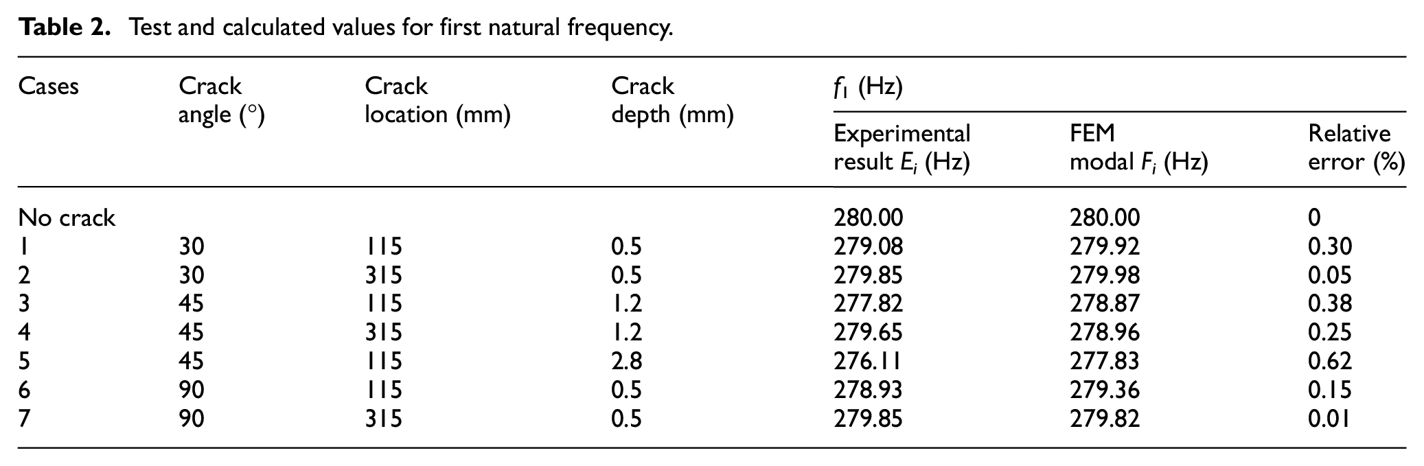
Test and calculated values for first natural frequency.

Cases	Crack angle (°)	Crack location (mm)	Crack depth (mm)	f₁ (Hz)
Cases	Crack angle (°)	Crack location (mm)	Crack depth (mm)	Experimental result E_i (Hz)	FEM modal F_i (Hz)	Relative error (%)
No crack				280.00	280.00	0
1	30	115	0.5	279.08	279.92	0.30
2	30	315	0.5	279.85	279.98	0.05
3	45	115	1.2	277.82	278.87	0.38
4	45	315	1.2	279.65	278.96	0.25
5	45	115	2.8	276.11	277.83	0.62
6	90	115	0.5	278.93	279.36	0.15
7	90	315	0.5	279.85	279.82	0.01

Table 3.

Test and calculated values for second natural frequency.

Cases	Crack angle (°)	Crack location (mm)	Crack depth (mm)	f₂ (Hz)
Cases	Crack angle (°)	Crack location (mm)	Crack depth (mm)	Experimental result E_i (Hz)	FEM modal F_i (Hz)	Relative error (%)
No crack				1506.30	1513.19	0.46
1	30	115	0.5	1512.98	1512.76	0.01
2	30	315	0.5	1507.34	1506.98	0.02
3	45	115	1.2	1512.16	1506.88	0.35
4	45	315	1.2	1499.17	1502.83	0.24
5	45	115	2.8	1507.50	1500.50	0.46
6	90	115	0.5	1511.92	1509.68	0.15
7	90	315	0.5	1504.14	1502.63	0.10

In Tables 2 and 3, the experimental and finite element results for the first and second natural frequencies of the hydraulic straight pipe are consistent. The relative errors for the first and second natural frequencies do not exceed 0.62% and 0.46%, respectively, which verifies the proposed finite element model.

Identification of slant crack location and depth

The occurrence of a crack in a hydraulic pipeline structure reduces the local stiffness and therefore directly affects the natural frequency of the system. Therefore, the natural frequency of a hydraulic piping system can be used as an input parameter to identify crack occurrence. The contour map method can be used to simultaneously identify the crack location and depth.^28,29 In this paper, slant cracks at 30°, 45° and 90° are considered as examples.

The first and second natural frequencies of the slant crack hydraulic straight pipe are used for crack identification. The contour plot method used to identify the slant crack parameters is described below.

A series of sample points within the range of the position and depth of the slant crack is selected, and the natural frequency of the cracked hydraulic straight pipe is calculated for crack angles of 30°, 45° and 90°.

Placing the origin of the coordinate system at the left end of the pipeline, the crack is located at l with a depth a. Let the relative depth of the slant crack α = a/D_e, and the relative location β = l_c/L. Then, the ith order (i = 1,2,…) natural frequency database of the hydraulic straight pipe is fitted using the crack relative position and crack depth as variables for the three crack angles to the damage surface.

A modal test is performed on the hydraulic straight pipe to obtain the first and second natural frequencies, and the measured natural frequency is used to determine the damage surface. Contour maps corresponding to the relative position and depth of the crack are drawn. The coordinates of the intersection of the two curves (or the centroid of the enclosed figure) represent the location and depth of the slant crack failure.

Figure 12 is a flow chart for identifying the slant crack failure of the hydraulic straight pipe using the finite element and contour plot methods and quantitatively diagnosing the position and depth of the slant crack.

Figure 12.

Slant crack fault diagnosis flowchart.

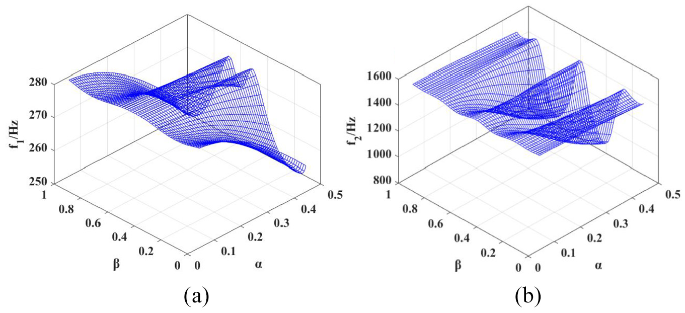
Figures 13 to 15 show the damage curved surface of the hydraulic straight pipe with slant cracks obtained using the proposed diagnostic method.

Figure 13.

Natural frequency damage curves of hydraulic straight pipe with 30° slant crack.

Figure 14.

Natural frequency damage curves of hydraulic straight pipe with 45° slant crack.

Figure 15.

Natural frequency damage curve of hydraulic straight pipe with 90° slant crack

After obtaining the damage surface, a modal test is performed on the straight pipe with slant cracks to obtain the first and second natural frequencies. The pre-second-order natural frequency is used as an input parameter to identify the crack location and depth in the pipeline. Table 4 shows the first and second natural frequencies of the uncracked and cracked pipe under six fault conditions.

Table 4.

Natural frequencies of pipeline under different working conditions.

Cases	Crack angle (°)	Crack location (mm)	Crack depth (mm)	Natural frequency (Hz)
Cases	Crack angle (°)	Crack location (mm)	Crack depth (mm)	f ₁	f ₂
No crack				280.00	1506.30
1	30	115	1.5	277.44	1512.76
2	30	315	1.5	279.55	1495.76
3	45	115	0.5	279.10	1512.76
4	45	315	0.5	279.85	1507.35
5	90	115	1.0	277.87	1510.66
6	90	315	1.0	279.70	1492.24

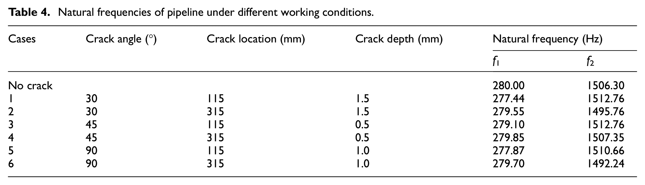
The pipeline structure remains highly symmetrical over the identification process. The two contour lines of the contour map have completely symmetrical intersections. Therefore, the intersection can be identified based on the side where the crack is located.³⁰ The seven sets of measured natural frequencies (including that of the uncracked pipeline) are used to draw a contour map of the first and second natural frequencies. Figures 16 and 17 show the contours in the coordinate system of the uncracked pipe.

Figure 16.

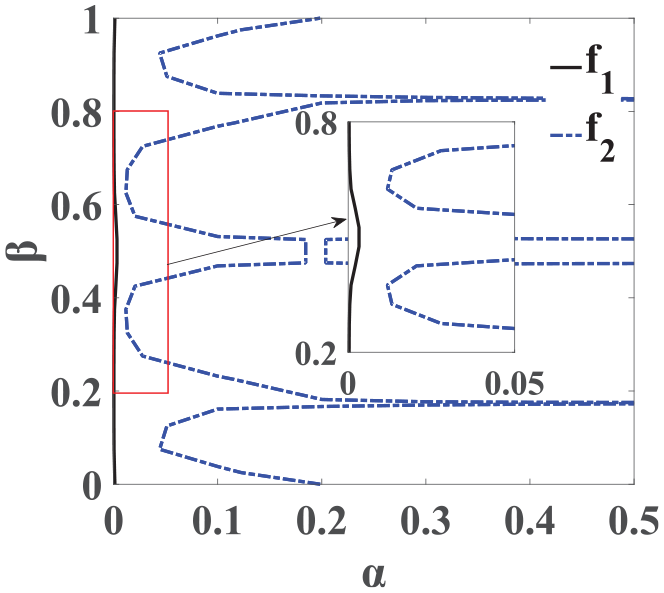
Contour diagram of natural frequency of uncracked pipeline.

Figure 17.

Contour diagram of natural frequency of crack failure state: (a) case 1; (b) case 2; (c) case 3; (d) case 4; (e) case 5 and (f) case 6.

Figure 16 shows that there are no possible intersections between the two contour lines of the contour map of the uncracked pipe. Therefore, the contour plot method can be used to diagnose cracks. The coordinates of the intersection (or the centre of mass of the enclosed figure) of the two curves in Figure 17 represent the position and depth of the slant crack. The actual crack parameters identified using the contour map method under different working conditions are shown in Table 5. The relative error calculation formula is

\frac{| A_{i} - D_{i} |}{A_{i}} \times 100 %

(29)

Table 5.

Identified parameters for slant cracks in hydraulic straight pipe.

Cases	Crack relative location (mm)		Relative error (%)	Crack relative depth (mm)		Relative error (%)
Cases	Actual value A_i	Diagnostic result D_i	Relative error (%)	Actual value A_i	Diagnostic result D_i	Relative error (%)
1	0.213	0.210	1.41	0.094	0.099	5.32
2	0.583	0.564	3.26	0.094	0.096	2.13
3	0.213	0.220	3.29	0.031	0.032	3.23
4	0.583	0.564	3.26	0.031	0.032	3.23
5	0.213	0.221	3.76	0.063	0.064	1.59
6	0.583	0.569	2.40	0.063	0.064	1.59

In Table 5, the relative errors in the slant crack position and depth do not exceed 3.76% and 5.32%, respectively. The actual and theoretical results for the slant crack position and depth are consistent. Therefore, the fault diagnosis method based on the proposed finite element model for diagonal cracks in an aero-hydraulic straight pipe is effective for detecting pipeline cracks in practice.

Conclusion

The vibration signals of aeronautical hydraulic straight pipes are non-linear, non-stationary and subject to strong noise interference, making it is difficult to obtain a prior diagnosis of slant crack faults. In this paper, a model-driven fault diagnosis method is proposed for slant cracks in aero-hydraulic straight pipes. Slant crack faults are identified, and the position and depth of slant cracks are quantified.

Fracture mechanics theory and the principle of strain energy release are used to derive an expression for the local flexibility coefficient of hydraulic straight pipes with slant cracks considering the influence of the shear force and the shear coefficient. A finite element model of an aeronautical hydraulic straight pipe with slant crack faults is established, and the effects of different angles, positions and depths of diagonal cracks on the local compliance coefficient are analysed.

The proposed finite element model is used to obtain the damage surface of the natural frequency of the hydraulic straight pipe. Modal experiments are performed on the hydraulic straight pipe with slant cracks to quantitatively identify slant crack faults at different locations and depths. The predicted and actual crack parameters are consistent, which verifies the accuracy and feasibility of the proposed method and provides a new approach for the quantitative diagnosis of cracks in aero-hydraulic pipelines.

Footnotes

Handling Editor: James Baldwin

Declaration of conflicting interests

The author(s) declared no potential conflicts of interest with respect to the research, authorship, and/or publication of this article.

Funding

The author(s) disclosed receipt of the following financial support for the research, authorship, and/or publication of this article: The research is supported by the National Natural Science Foundation of China (Grant No. 51775257).

ORCID iDs

Dou Jinxin

Yu Xiaoguang

References

Zhang

Kong

Huang

, et al. Fluid-structure-interaction analysis of an aero hydraulic pipe considering friction coupling. IEEE Access 2019; 7: 26665–26677.

Lin

Zhou

, et al. Literature review on vibration mechanism and fault diagnosis of the pipe. Mach Tool Hydraulics 2013; 41(1): 163–164, 141.

Gao

Zhao

, et al. Fault diagnosis and location of the aero-engine hydraulic pipeline based on Kalman filter. Adv Mech Eng 2017; 9(12): 168781401774281.

Gao

Tong

, et al. Research of fault diagnosis method of hydraulic pipeline cracks based on HHT. Comput Eng Appl 2016; 52(20): 221–226.

Zhu

Wang

Yin

, et al. Spectral element method for vibration analysis of three- dimensional pipes conveying fluid. Int J Mech Mater Des 2019; 15(2): 345–360.

Pavlou

Correia

. Dynamic response of pipelines under impact and harmonic loading. Proc Inst Civ Eng 2019; 172(MA1): 15–22.

Gao

Zhai

Han

. Dynamic response analysis of aero hydraulic pipeline system under pump fluid pressure fluctuation. Proc Inst Mech Eng 2019; 233(5): 1585–1595.

Gao

Zhai

, et al. Vibration and damping analysis of aerospace pipeline conveying fluid with constrained layer damping treatment. Proc Inst Mech Eng 2018; 232(8): 1529–1541.

Gao

Zhai

Yan

, et al. A model reduction approach for the vibration analysis of hydraulic pipeline system in aircraft. Aerosp Sci Technol 2016; 49: 144–153.

10.

Zhai

Liu

, et al. Dynamic response of pipeline conveying fluid to random excitation. Nucl Eng Des 2011; 241(8): 2744–2749.

11.

Ouyang

Gao

Yang

, et al. Modal analysis of the aircraft hydraulic-system pipeline. J Aircraft 2012; 49(4): 1168–1174.

12.

Wang

Liu

Huo

, et al. Identification of leakage degree of hydraulic pipeline based on probabilistic neural network. Mach Tool Hydraulics 2020; 48(4): 159–164.

13.

Quan

Kong

Bin

, et al. Research status and trends on fluid-structure interaction vibration mechanism and control of hydraulic pipeline. J Mech Eng 2015; 51(18): 175–183.

14.

Yang

Wang

, et al. Dynamic characteristics of cracked uncertain hollow-shaft. Mech Syst Signal Process 2019; 124: 36–48.

15.

Wang

Wei

, et al. Initial crack propagation and the influence factors of aircraft pipe pressure. Materials 2019; 12(19): 3098.

16.

Bao

Liang

. Nonlinear dynamic characteristics of a cracked pipe conveying fluid under two-end elastic supports. J Vib Shock 2017; 36(1): 70–74, 87.

17.

Bao

Liang

. Dynamic characteristics of a cracked pipe conveying fluid with both elestically supported ends. J Vib Shock 2016; 35(7): 220–224.

18.

Liu

Barkey

. Frequency error based identification of cracks in beam-like structures. J Mech Sci Technol 2017; 31(10): 4657–4667.

19.

Chen

. Three-steps-meshing based multiple crack identification for structures and its experimental studies. Chin J Mech Eng 2013; 26(2): 400–405.

20.

Sinou

. On the use of non-linear vibrations and the anti-resonances of Higher-Order Frequency Response Functions for crack detection in pipeline beam. Mech Res Commun 2012; 43: 87–95.

21.

Wang

. Finite element method. Beijing: Tsinghua University Press, 2010.

22.

Wang

Qiu

. Research on stability reliability of pipe conveying fluid based on finite element method. J Aerosp Power 2017; 32(12): 2903–2909.

23.

Dimarogonas

Paipetis

. Analysis methods in rotor dynamics. Essex: Applied Science Publishers, 1983.

24.

Cowper

. The shear coeficient in Timoshenko’s beam theory. J Appl Mech 1966; 33(3): 393–398.

25.

Papadopoulos

. The strain energy release approach for modeling cracks in rotors: a state of the art review. Mech Syst Signal Process 2008; 22(4): 763–789.

26.

Murigendrappa

Maiti

Srirangarajan

. Experimental and theoretical study on crack detection in pipes filled with fluid. J Sound Vib 2004; 270(4–5): 1013–1032.

27.

Chen

, et al. Pipe crack identification based on finite element method of second generation wavelets. Mech Syst Signal Process 2010; 24(2): 379–393.

28.

Feng

Zhou

. Vibration analysis and crack identification of a cantilever pipe with a circumferential part-through crack. J Vib Shock 2011; 30(4): 21–25.

29.

Wang

Chen

. Daubechies wavelet finite element method and genetic algorithm for detection of pipe crack. Nondestruct Test Eva 2011; 26(1): 87–99.

30.

Gao

Zhang

, et al. Pipe crack quantitative identification based on the change of the local flexibility. J Vib Meas Diagn 2015; 35(6): 1184–1189, 1207.

Model-driven fault diagnosis of slant cracks in aero-hydraulic straight pipes

Abstract

Keywords

Introduction

Establishment of finite element model

Numerical calculation and experimental verification

Calculation of local flexibility coefficient of hydraulic straight pipe with slant crack

Modal experiment verification

Identification of slant crack location and depth

Conclusion

Footnotes

Declaration of conflicting interests

Funding

ORCID iDs

References