Implementation of micropolar fluids model and hydrodynamic behavior analysis using user-defined function in FLUENT

Abstract

Micropolar fluids commonly represent the complex fluids with microstructure, for example, animal blood and liquid crystals. To understand the behavior of micropolar fluids and the role of micropolar parameters, different micropolar fluids models were implemented by user-defined function in the FLUENT software. The correctness of user-defined function programs was verified comparing to the analytical solution in the Poiseuille flow. Then, the hydrodynamic behavior was analyzed in the Poiseuille flow with a moving particle, slider bearing, and dam break. Numerical results show that microrotation viscosity weakens translational velocity while enhances the pressure of micropolar fluids, in addition, microrotation velocity decreases with the increase in angular viscosity.

Introduction

Researchers gradually realize that the classical fluid has a limitation in describing complex fluids, for example, polymeric fluids, liquid crystals, colloidal systems, suspensions, and emulsions, as the local structure and microrotation of the fluid element is not considered especially at micro- and nanoscales. ¹ To describe the effect of microstructure, micropolar fluid theory was established by Eringen^2,3 and Eringen and Suhubi. ⁴ Physically, micropolar fluids may represent the fluids consisting of rigid, randomly oriented, or spherical particles suspended in a viscous medium.

As the equations of micropolar fluids are highly nonlinear, various methods^5,6 have been presented to investigate its solutions. Among them, the behavior of microchannel fluids was described using the finite difference method and experimentally verified by Papautsky et al. ¹ They found that the numerical results based on micropolar fluids predicted experimental data better than classical Navier–Stokes theory. Routh ⁷ mentioned that finite difference method needs lots of calculation and computer programming to get the almost same result compared to direct integration method. In his study, computational fluid dynamics (CFD) analysis was also presented to justify pressure profile obtained by direct numerical method in infinitely long/short journal bearings. Asadi et al. ⁸ developed finite element formulation for numerical analysis on the behaviors of the blood flowing through a stenosed artery, and the same method was applied for energy transfer analysis in a lid-driven porous square container filled with micropolar fluids. ⁹ Besides, the homotopy perturbation method (HPM) was proposed to derive the solution of nonlinear equations of micropolar fluids flowing in a permeable channel subjected to chemical reaction, ¹⁰ and the numerical solution by four-order Runge–Kutta method was presented to verify the accuracy. Boukrouche et al. ¹¹ proved the existence and uniqueness solution for two-dimensional (2D) domain with micropolar fluids by theoretical analysis assuming that velocity field satisfies the Tresca friction boundary conditions while microrotation field satisfies non-homogeneous the Dirichlet boundary conditions. And the regularity criterion of weak solutions to three-dimensional (3D) incompressible micropolar fluid equations in terms of the pressure condition was obtained by Liu. ¹² In addition, some developed solutions based on micropolar fluid equations were investigated, for example, the mathematics analysis of thermophoresis theory, ¹³ the approximate solution of compressible viscous and heat-conducting micropolar fluids, ¹⁴ and closed form of the Poiseuille flow subjected to electromagnetic field under the linear slip boundary conditions. ¹⁵

The demand of engineering applications in medicine, mechanical engineering, and chemical industry makes micropolar fluids be a focus and get more and more attention. As a result, numerous research works have been emerged, for example, a novel application of bio-inspired computational heuristic paradigm ¹⁶ and the investigation of surface roughness and squeeze film lubrication problems between conical bearings. ¹⁷ Khanukaeva et al. ¹⁸ devoted to the application of cell model combined a swarm of solid cylindrical particles with porous layer involving micropolar fluids, which the effect of particle volume fraction, permeability parameter, and micropolarity number on the hydrodynamic permeability of the membrane was discussed.

Limited by the complex differential equations of micropolar fluids, it is difficult to obtain the pure solution of the corresponding model. In this study, we introduced the user-defined function (UDF) to obtain the solution of micropolar fluid model and analyzed its hydrodynamic behaviors. First, the theory of micropolar fluids and the description of UDF were presented. Next, the implementation of micropolar fluid model by UDF programs was validated comparing to the analytical solution in the Poiseuille flow. Then, the influence of micropolar parameters on the physical quantities—that is, translational velocity, microrotation velocity, and pressure—was investigated in different micropolar fluid models. In the end, there are conclusions and prospects.

Micropolar fluids equations

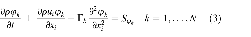
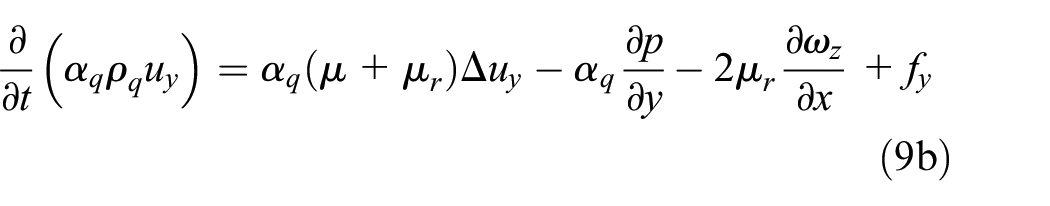
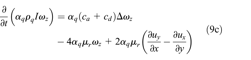
The governing equations of micropolar fluids regardless of the temperature variation are as follows referred to Petrosyan ¹⁹ and Lukaszewicz’s ²⁰ books

$$\frac{D\rho }{\mathrm{Dt}}=-\rho \nabla ·\mathbf{u}$$

(1a)

$$\begin{array}{c}\multicolumn{1}{c}{\rho \frac{D\mathbf{u}}{\mathrm{Dt}}=-\nabla p+(\lambda +\mu -{\mu }_r)\nabla \mathrm{div}\mathbf{u}}\\ +(\mu +{\mu }_r)\mathrm{\Delta }\mathbf{u}+2{\mu }_r\mathrm{rot}\mathbf{\omega }+\rho \mathbf{f}\hfill \end{array}$$

(1b)

$$\begin{array}{c}\multicolumn{1}{c}{\rho I\frac{D\mathbf{\omega }}{\mathrm{Dt}}=2{\mu }_r(\mathrm{rot}\mathbf{u}-2\mathbf{\omega })+(c_0+c_d-c_a)\nabla \mathrm{div}\mathbf{\omega }}\\ +(c_a+c_d)\mathrm{\Delta }\mathbf{\omega }+\rho \mathbf{\tau }\hfill \end{array}$$

(1c)

where $\rho$ and $p$ represent the density and the pressure, respectively, $\lambda$ and $\mu$ are the second viscosity coefficient and the dynamic Newtonian viscosity, respectively. ${\mu }_r$ represents the dynamic microrotation viscosity, and $c_0$ , $c_a$ , and $c_d$ are the constants called the coefficient of angular viscosity. $\mathbf{f}$ and $\mathbf{\tau }$ represent the body force per unit mass and the body torque per unit mass, respectively, $I$ is a scalar called the microinertia coefficient, and $D/\mathrm{Dt}$ denotes the material derivative.

Compared with the classical fluid, there is one more physical quantity named the angular velocity $\mathbf{\omega }$ which can describe the microrotation of the microstructure, so one more conservation equation of angular momentum is needed. Notice that if $\mathbf{\tau }\mathbf{,}\mathbf{\omega }$ , and viscosity coefficients $c_0$ , $c_a$ , $c_d$ , and ${\mu }_r$ are zero, then equation (1) reduces to the field equations of classical fluids

$$\frac{D\rho }{\mathrm{Dt}}=-\rho \nabla ·\mathbf{u}$$

(2a)

$$\rho \frac{D\mathbf{u}}{\mathrm{Dt}}=-\nabla p+(\lambda +\mu )\nabla \mathrm{div}\mathbf{u}+\mu \mathrm{\Delta }\mathbf{u}+\rho \mathbf{f}$$

(2b)

Numerical method

Finite volume method (FVM) is an important and popular class of discretization numerical method used in CFD, which has fine conservation in solving differential equations. The thought of FVM is that the differential equations to be calculated are integrated in a control volume and a certain time interval after the computational region was divided into a series of control volume units and each of which was represented by a node information. FVM has good adaptability to the grid; therefore, it can solve complex engineering problems well and perfectly combine with the finite element method in fluid–solid coupling analysis. As FLUENT can solve the transport equations for an arbitrary user-defined scalar (UDS) by UDF, therefore, the investigation of the hydrodynamic behaviors of micropolar fluids was implemented using UDF compiled through FLUENT in this study. Here, C language and UDF—for example, DEFINE_UDS_UNSTEADY, DEFINE_PROPERTY, DEFINE_DIFFUSIVITY, and DEFINE_SOURCE—are prerequisite to prepare the solution program of differential equations with different boundary conditions.

For an arbitrary scalar ${\phi }_k$ , FLUENT solves the equation in the following form

$$\frac{\partial \rho {\phi }_k}{\partial t}+\frac{\partial \rho u_i{\phi }_k}{\partial x_i}-{\mathrm{\Gamma }}_k\frac{{\partial }^2{\phi }_k}{\partial x_i^2}=S_{{\phi }_k}k=1,\dots ,N$$

(3)

where ${\mathrm{\Gamma }}_k$ and $S_{{\phi }_k}$ are the diffusion coefficient and the source term supplied for each of scalar equation. Note that ${\mathrm{\Gamma }}_k$ is defined as a tensor in the case of anisotropic diffusivity; hence, the diffusion term is $\nabla ·({\mathrm{\Gamma }}_k·{\phi }_k)$ .

For multiphase flows, FLUENT solves transport equations for two types of scalars: per phase and mixture. For an arbitrary $k$ scalar in the first phase, denoted by ${\phi }_l^k$ , FLUENT solves the transport equation inside a volume occupied by the first phase

$$\begin{array}{c}\multicolumn{1}{c}{\frac{\partial {\alpha }_l{\rho }_l{\phi }_l^k}{\partial t}+\nabla ·({\alpha }_l{\rho }_l{\mathbf{u}}_l{\phi }_l^k-{\alpha }_l{\mathrm{\Gamma }}_l^k\nabla {\phi }_l^k)}\\ =S_l^{k}k=1,\dots ,N\hfill \end{array}$$

(4)

where ${\alpha }_l$ , ${\rho }_l$ , and $u_l$ are the volume fraction, the physical density, and the velocity of the first phase, respectively. ${\mathrm{\Gamma }}_l^k$ and $S_l^k$ represent the diffusion coefficient and the source term, respectively. In this case, the scalar ${\phi }_l^k$ is associated only with one phase and is considered an individual field variable of the first phase.

Numerical examples

Poiseuille flow

The Poiseuille flow can be considered as the micropolar fluids in the analysis of blood flow as the microstructure can vividly represent the existence of erythrocyte flowing with the blood. Therefore, the study of flow behavior under a certain pressure drop can provide a reference for the analysis of blood movement, including the speed of metabolism.

Provided that the fluid is incompressible and in steady state, with no external force, it yields from equation (1)

$$\mathrm{div}\mathbf{u}=0$$

(5a)

$$-(\mu +{\mu }_r)\mathrm{\Delta }\mathbf{u}+(\mathbf{u}·\nabla )\mathbf{u}+\nabla p=2{\mu }_r\mathrm{rot}\mathbf{\omega }$$

(5b)

$$\begin{array}{c}-(c_a+c_d)\mathrm{\Delta }\mathbf{\omega }+I(\mathbf{u}·\nabla )\mathbf{\omega }\hfill \\ -(c_0+c_d-c_a)\nabla \mathrm{div}\mathbf{\omega }+4{\mu }_r\mathbf{\omega }=2{\mu }_r\mathrm{rot}\mathbf{u}\hfill \end{array}$$

(5c)

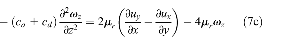
We simplified the Poiseuille flow as 2D flow between parallel plates in the direction of the x-axis with the absence of mass forces and moments. Herein, change equations (5a)–(5c) in the form of UDS transport equations, it obtains

$$(\mu +{\mu }_r)\frac{{\partial }^2{u}_x}{\partial y^2}=\frac{\partial p}{\partial x}-2{\mu }_r\frac{\partial {\omega }_z}{\partial y}$$

(6a)

$$(c_a+c_d)\frac{{\partial }^2{\omega }_z}{\partial y^2}=2{\mu }_r(2{\omega }_z+\frac{\partial u_x}{\partial y})$$

(6b)

For comprehensive understanding of Poiseuille flow, one can refer to Beneš et al.’s ²¹ study, it provided the global existence and uniqueness result for generalized time-dependent Poiseuille solution by means of semi-discretization in time.

Poiseuille flow

The simplified 2D Poiseuille flow is shown in Figure 1 with $2h=4\mathrm{mm}$ , computational domain is divided by quadrilateral mesh, and element size is 0.1 mm. Set the upper and lower boundary conditions as no-slip boundary, the left as the pressure inlet and the right as the pressure outlet with $\partial p/\partial x=-2\rho \mu /h^2=1000\mathrm{Pa}/\mathrm{m}$ . Fluid density $\rho =1\mathrm{kg}/{\mathrm{m}}^3$ and dynamic viscosity $\mu =0.002\mathrm{Pa}·\mathrm{s}$ are considered, and micropolar parameters ${\mu }_r=2.2\times {10}^{-4}\mathrm{Pa}·\mathrm{s}$ , ${\mu }_r=1.05\times {10}^{-4}\mathrm{Pa}·\mathrm{s}$ , ${\mu }_r=2\times {10}^{-5}\mathrm{Pa}·\mathrm{s}$ , $c_a+c_d=8\times {10}^{-9}\mathrm{N}·\mathrm{s}$ , $c_a+c_d=2\times {10}^{-9}\mathrm{N}·\mathrm{s}$ , and $c_a+c_d=8.8\times {10}^{-10}\mathrm{N}·\mathrm{s}$ are proposed, respectively, to investigate the variation of hydrodynamic behavior.

Figure 1.

Schematic of Poiseuille flow.

As shown in Figure 2, translational velocity in the x-direction is parabolic along the y-coordinate. It can be seen from the local enlargement diagram that the numerical solution obtained UDF program is in good agreement with analytical solution calculated by MATLAB, which fully demonstrates the correctness of FVM in calculating differential equations of micropolar fluids. Comparing the translational velocity under different microrotation viscosities, it can be known that owing to the existence of microstructure, the translational velocity profile is shown to deviate from classical parabolic profile, which is the same conclusion in Delhommelle and Evan’s ²² study. In addition, with the decrease in the microrotation viscosity from $2.2\times {10}^{-4}$ to $2\times {10}^{-5}\mathrm{Pa}·\mathrm{s}$ , the velocity distribution in the x-direction is closer to that of classical fluids $({\mu }_r=0)$ with the deviation from 9.59% to 0.98%, which indicates that the existence of microrotation viscosity will weaken the translational velocity, and at the same time, the kinetic energy of the fluid is weakened to a certain extent. It may infer that when the concentration of blood admixture such as drugs and macromolecular polymers increases, it will slow down the blood movement and the metabolism.

Figure 2.

Translational velocity with different microrotation viscosities.

We can see that the effect of angular viscosity coefficient on microrotation velocity is obvious from Figure 3, the distribution along the central of y-coordinate is centrosymmetric, and the numerical result of microrotation velocity is well consistent with analytical solutions obtained by MATLAB as the angular viscosity is $c_a+c_d=8\times {10}^{-9}\mathrm{N}·\mathrm{s}$ . The results show that with the increase in the coefficient of angular viscosity, the absolute value of microrotation velocity decreases gradually from 85.12 s⁻¹ to 12.22 s⁻¹, that is, the increase in angular viscosity hinders the occurrence of microrotation and weakens the generation of fluid vortices, leading to the gradual evolution of classical fluids into micropolar fluids. Combining with Figure 2, it can be seen that angular viscosity coefficient is a restriction to microrotation velocity, the translational velocity is confined by the microrotation viscosity, and the translational velocity profile is not affected by the angular viscosity, which has similar characteristics compared to Travis’s ²³ and Radzyner’s ²⁴ study.

Figure 3.

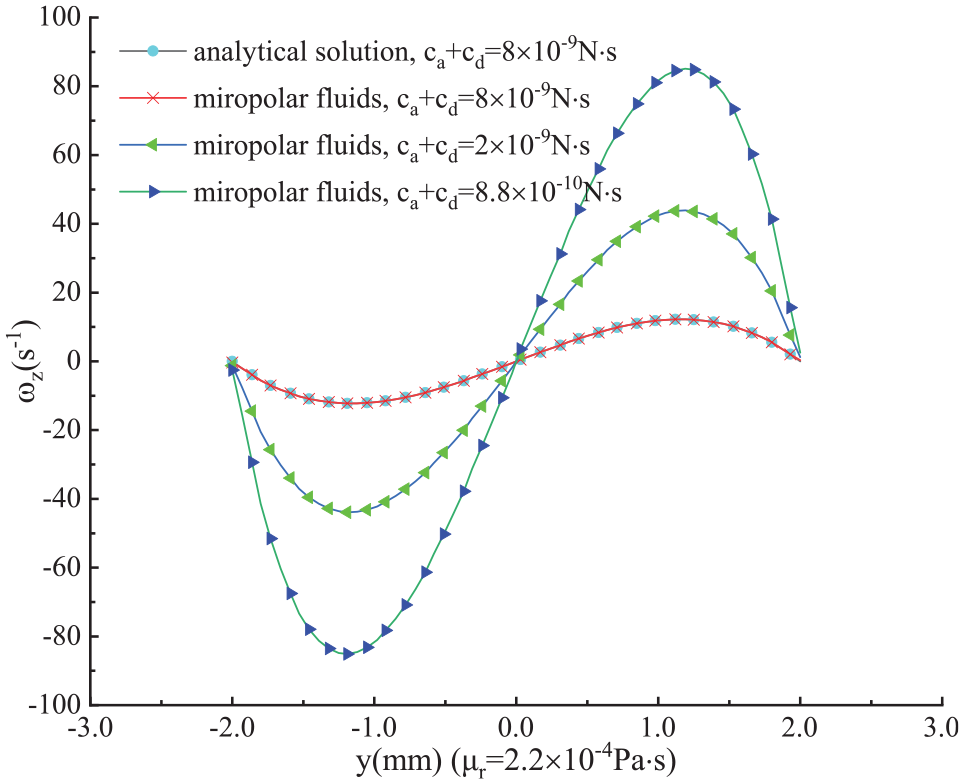
The effect of angular viscosity on microrotation velocity.

Poiseuille flow with a moving particle

Studying the behavior of moving particles in micropolar fluids is significant in chemistry and biology, such as moving drugs in blood. In this part, we do not directly consider the coupling between the particle and fluids. We use dynamic boundary conditions, that is, dynamic grid technology, to realize the movement of a particle in the fluid. The coupling mechanism between particles and fluids will be considered in the next study. And readers can refer to Sherief et al.’s^25,26 research to understand the calculation of real particles and micropolar fluid system, which including coupling relationship, boundary condition setting, and so on.

The calculation model is divided by triangular grids as shown in Figure 4 with the average mesh quality 0.944. In FLUENT, the evaluation index of mesh quality is between 0 and 1, that is, the closer the grid quality is to 1, the higher the accuracy of the calculation results. Physical quantities $\rho =1050\mathrm{kg}/{\mathrm{m}}^3$ and $\mu =0.002\mathrm{Pa}·\mathrm{s}$ are adopted, and boundary conditions are same as the above model beside the moving particle created by the dynamic mesh. Thus, the variation of microrotation velocity at different times is calculated under the condition of ${\mu }_r=2.2\times {10}^{-4}\mathrm{Pa}·\mathrm{s}$ and $c_a+c_d=8\times {10}^{-9}\mathrm{N}·\mathrm{s}$ . The results also compared to the numerical solution of classical fluids as shown in Figure 7.

Figure 4.

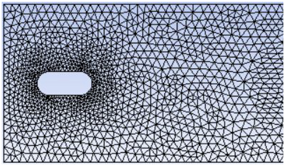
The calculation mesh.

It presents the particle position at $t=0.25\mathrm{s}$ , $t=0.5s$ , $t=0.75s$ , and $t=1s$ with the local enlarged detail of the variation of microrotation velocity around the particle at $t=1s$ in Figure 5. Due to the application of dynamic boundary conditions to simulate the movement of a particle with a constant velocity 0.08 m/s, it can be seen that when t = 0.25 s, the absolute value of microrotation speed is small. As time goes on, the disturbance caused by a moving particle in micropolar fluids increases and tends to be stable. As mentioned above, the microrotation velocity distributes centrosymmetrically, which can be approximately explained from contour legend in this simulation. The local enlargement shows a detailed distribution of microrotation velocity around the particle. On both sides of the upper and lower walls, microrotation speed is approximately equal but in opposite direction. Interestingly, the distribution of microrotation velocity on the upper and lower sides of the particle is opposite, that is, negative microrotation velocity on the upper side and positive microrotation on the lower side, but this distribution just balances the microrotation velocity on both sides of upper and lower walls. Similarly, the turbulence caused by the change of particle surface at the tail of a moving particle can still be reflected from the local enlarged image. The detailed study of the streamline style produced by a heavy particle in the Poiseuille flow with Newtonian fluids can refer to Liu et al. ²⁷

Figure 5.

Microrotation velocity contour at different times.

Figure 6 shows the change of microrotation velocity along y-direction at the right end of the model. It can be seen that microrotation velocity still distributes centrosymmetrically along the central axis of flow direction, but because of the existence of a moving particle, the change of curve is not smooth. As time goes on, the particle gradually moves to the right side of the model; hence, the absolute value of microrotation velocity becomes larger and larger.

Figure 6.

Variations of microrotation velocity at different moments.

Figure 7 displays a comparison of translational velocity at the right side of the model along y-coordinate between micropolar fluids and classical fluids when $t=1s$ . It can be seen that the distribution of translational velocity is no longer symmetrical strictly, which may be due to the change of the flow characteristics caused by a moving particle. Also it shows that the translational velocity of micropolar fluids is slightly lower than that of classical fluids with the largest deviation of 4.76% at y = 0.1 mm due to the effect of microstructure with parameters ${\mu }_r=2.2\times {10}^{-4}\mathrm{Pa}·\mathrm{s}$ and $c_a+c_d=8\times {10}^{-9}\mathrm{N}·\mathrm{s}$ ; this phenomenon matches with Hoffmann et al.’s ²⁸ conclusion on the difference of particle drag in classical fluids and micropolar fluids.

Figure 7.

The effect of micropolar parameters on translational velocity.

Slider bearing

Lubricant is widely used in bearing industry as it can provide hydraulic pressure between two objects to reduce the abrasion caused by relative motion. But the lubricant will be contaminated gradually with foreign particles or worn out dust-metal particles in industrial application. At this point, the solution of pressure based on classical fluids theory will deviate from the actual value. Hence, the hydrodynamic analysis based on micropolar fluid theory is more reasonable to represent lubricants containing additives.

For simplicity, we confine 2D slider bearing to investigate the solution of the differential equations of lubricants, which is shown as follows in the form of UDS transport equations

$$-(\mu +{\mu }_r)(\frac{{\partial }^2{u}_x}{\partial x^2}+\frac{{\partial }^2{u}_x}{\partial y^2})=2{\mu }_r\frac{\partial {\omega }_z}{\partial y}-\frac{\partial p}{\partial x}$$

(7a)

$$-(\mu +{\mu }_r)(\frac{{\partial }^2{u}_y}{\partial x^2}+\frac{{\partial }^2{u}_y}{\partial y^2})=2{\mu }_r\frac{\partial {\omega }_z}{\partial x}-\frac{\partial p}{\partial y}$$

(7b)

$$-(c_a+c_d)\frac{{\partial }^2{\omega }_z}{\partial z^2}=2{\mu }_r(\frac{\partial u_y}{\partial x}-\frac{\partial u_x}{\partial y})-4{\mu }_r{\omega }_z$$

(7c)

The lubrication films to be analyzed are assumed to comply with usual assumptions: ²⁹ (1) flow is incompressible and laminar, vortex and turbulence do not occur anywhere in the film; (2) body forces are neglected, that is, gravitational force and magnetic field are assumed to be negligible; (3) film is sufficiently thin compared with the length and span of the bearing to allow the curvature of lubricant film to be ignored; and (4) no-slip on bearing surfaces.

We consider the non-dimensional parameters

$$\begin{array}{c}\overline{x}=\frac{x}{B},\overline{y}=\frac{y}{h_1},{\overline{y}}_0=\frac{y}{h_0},h_0=\frac{(h_1+h_2)}{2},\overline{\mathbf{u}}=\frac{\mathbf{u}}{U}\hfill \\ \overline{\omega }=\frac{\omega h_1}{U},\overline{p}=\frac{{\mathrm{ph}}_0^2}{\mu \mathrm{UB}},\overline{z}=\frac{z}{b},L=\frac{h_0}{l},\hfill \\ N^2=\frac{{\mu }_r}{\mu +{\mu }_r},l^2=\frac{c_a+c_d}{4\mu }\hfill \end{array}$$

and the relationships

$$\begin{array}{c}{\alpha }_1=\frac{{\mu }_{r}U}{\mathrm{Bp}},{\alpha }_2=\frac{{\mu }_r\mathrm{UB}}{h_1^{2}p},{\alpha }_3=\frac{\mu \mathrm{UB}}{h_0^{2}p},{\beta }_1=\frac{2{\mu }_{r}U}{h_{1}p},\hfill \\ {\beta }_2=\frac{\mu U{B}^2}{h_0^2{h}_{1}p},{\beta }_3=\frac{4\mu {\mathrm{Uh}}_0^2}{h_{1}p{b}^2}\hfill \end{array}$$

Hence, the non-dimensional equations can be presented as follows

$$-\frac{1}{N^2}({\alpha }_1\frac{{\partial }^2{\overline{u}}_{\overline{x}}}{\partial {\overline{x}}^2}+{\alpha }_2\frac{{\partial }^2{\overline{u}}_{\overline{x}}}{\partial {\overline{y}}^2})=2{\alpha }_2\frac{\partial {\overline{\omega }}_{\overline{z}}}{\partial \overline{y}}-{\alpha }_3\frac{\partial \overline{p}}{\partial \overline{x}}$$

(8a)

$$-\frac{1}{N^2}({\alpha }_1\frac{{\partial }^2{\overline{u}}_{\overline{y}}}{\partial {\overline{x}}^2}+{\alpha }_2\frac{{\partial }^2{\overline{u}}_{\overline{y}}}{\partial {\overline{y}}^2})={\beta }_1\frac{\partial {\overline{\omega }}_{\overline{z}}}{\partial \overline{x}}-{\beta }_2\frac{\partial \overline{p}}{\partial \overline{y}}$$

(8b)

$$-\frac{1}{L^2}{\beta }_3\frac{{\partial }^2{\overline{\omega }}_{\overline{z}}}{\partial {\overline{z}}^2}=2{\alpha }_1\frac{\partial {\overline{u}}_{\overline{y}}}{\partial \overline{x}}-{\beta }_1\frac{\partial {\overline{u}}_{\overline{x}}}{\partial \overline{y}}-2{\beta }_2{\overline{\omega }}_{\overline{z}}$$

(8c)

where $B=15\mathrm{m}$ , $h_0=1.6\mathrm{mm}$ , $h_1=2.1889\mathrm{mm}$ , $h_2=1\mathrm{mm}$ , $U=1\mathrm{m}/\mathrm{s}$ in this example shown in Figure 8, and $b$ is the unit length in z-dimension, and parameters $N^2$ and $L$ are considered as the coupling number and the characteristic length of micropolar fluids, respectively. The parameter $L$ can be taken as a characterization of the interaction between the fluids with bearing geometry, $N^2$ is regarded as the parameter coupling the linear momentum and angular momentum equations, and restrictions require that $0\le N\le 1$ from Eringen. ² The larger $N^2$ means that the individuality of substructure becomes more significant. When $N$ approaches zero or $L$ approaches infinity, the micropolarity of fluids is lost, and then control equations degenerate to the classical ones. ⁵

Figure 8.

Slider bearing configuration. ³⁰

We set the bearing and slider boundary conditions as the wall, the left as the pressure inlet, and the right as the pressure outlet with the initial vale 0. Select the lubricant parameter $\rho =922.5\mathrm{kg}/{\mathrm{m}}^3$ and $\mu =0.16\mathrm{Pa}·\mathrm{s}$ , and lubricant film is thin enough about $1/{10}^4$ times to the size of bearing, thus the change of micropolar parameters will produce obvious hydrodynamic characteristics.^30,31 The micropolar parameters used in the comparison calculation are shown in Table 1; computational domain is divided into triangular mesh with a minimum element size of 0.2 mm.

Table 1.

Micropolar parameters in calculation of slider bearing.

$N^2=\frac{{\mu }_r}{\mu +{\mu }_r}$	0.4	0.2	0.1	0.01
${\mu }_r(\mathrm{Pa}·s)$	0.107	0.04	0.018	0.0016
$l^2=\frac{c_a+c_d}{4\mu }(m^2)$	–	2.56 × 10−6	0.64 × 10−7	0.284 × 10−7
$L=\frac{h_0}{l}$	–	1	2	3
$c_a+c_d(N·s)$	–	1.638 × 10−6	0.41 × 10−6	0.182 × 10−6

Figure 9 presents the variation of lubricant pressure along the slider side with different microrotational viscosities under the influence of moving slider. At the same viscosity, the pressure along x-direction increases first and then decreases, which has the same trend with Hanoca and Ramakrishna’s study. ³⁰ And the pressure has a maximum value at a certain position in the x-direction, which indicates that there is no pressure flow velocity but only shear flow velocity. Also from the figure, the higher microrotation viscosity, which may have some certain relationships with the additive concentration, the higher lubricant pressure, and the maximum of pressure at $c_a+c_d=1.638\times {10}^{-6}\mathrm{N}·\mathrm{s}$ and ${\mu }_{\mathrm{r}}=0.107\mathrm{Pa}·\mathrm{s}$ are approximately two times than those of calculated in classical fluids. It may infer that the increased additive concentration will decrease the microrotation viscosity thus weaken the lubricant pressure combined with practice experience. In other words, the hydraulic pressure is an increase function of microrotation viscosity and is always greater than the results of classical fluids, which are consistent with Khonsari and Brewe’s ³² conclusion.

Figure 9.

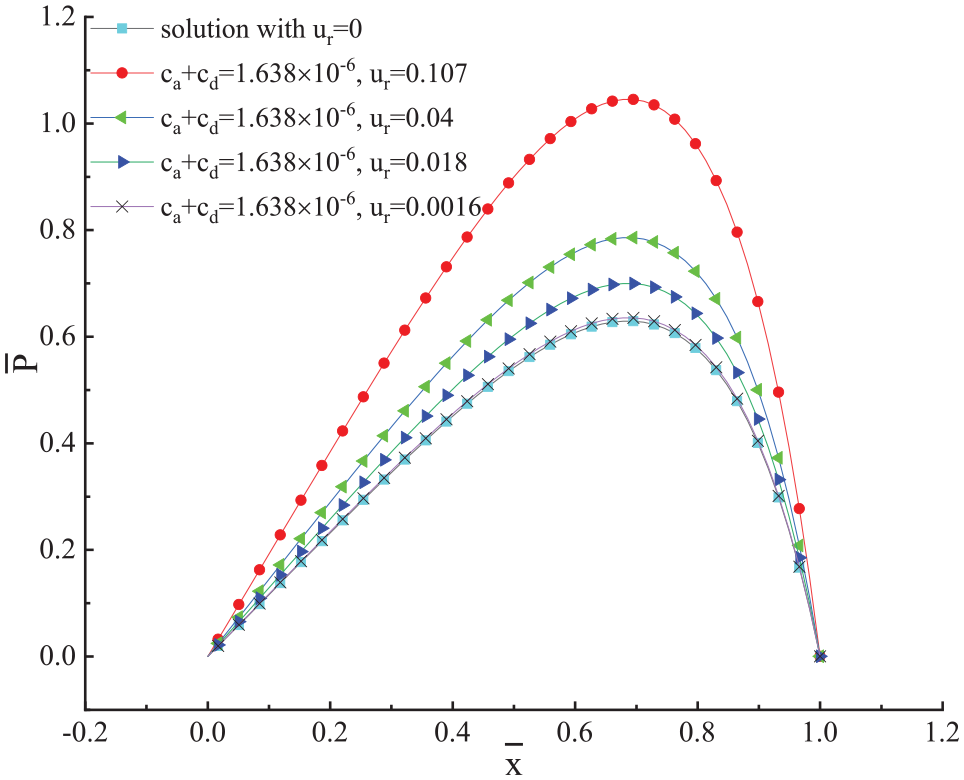
The effect of microrotation viscosity on pressure.

Figure 10 displays the distribution of microrotation velocity along y-coordinate at the left side of the slider bearing with the change of micropolar parameters. The overall distribution in the y-direction is parabolic but is different from that of in Poiseuille flow. Figure 10(a) presents the effect of microrotation viscosity on microrotation velocity, which shows that microrotation velocity is an increasing function of microrotation viscosity when angular viscosity is constant. And a similar conclusion can be obtained from Figure 10(b), that is, microrotation velocity increases with the increase in angular viscosity. But the difference of microrotation velocity caused by two parameters is about one order of magnitude, which illustrates that the effect of angular viscosity on microrotation velocity is greater than that of microrotation viscosity.

Figure 10.

Variation of microrotation velocity with different micropolar viscosities. (a) Variation of microrotation velocity with microrotation viscosity when angular viscosity $c_a+c_d$ is constant and (b) Variation of microrotation velocity with angular viscosity when microrotation viscosity ${\mu }_r$ is constant.

Figure 11 shows the variation of resultant velocity and x-velocity at the center position of x-axis along y-direction, which the velocity decreases with the increase in y-coordinate and the velocity on the side of moving slider is the largest. The comparison between resultant velocity and x-velocity in both classical fluids and micropolar fluids is presented in Figure 11(a). It can be seen that, as lubricant film is extremely narrow in slider bearing, the deviations between resultant velocity and x-velocity are averagely 2.02% and 2.30% in classical fluids and micropolar fluids, respectively, which means that the component of y-velocity is negligible. It can also be found that, as microstructure is taken into account, the velocity distributed along y-coordinate in micropolar fluids is gentler than that of in classical fluids. Furthermore, as we can know from Figure 11(b), with the decrease in microrotation viscosity, x-velocity is gradually close to the values calculated in classical fluids. It is interesting that the trend does not start from one direction but from both sides of the solution of classical fluids at the same time. This phenomenon demonstrates that there is a certain position in y-direction where the velocity is a constant.

Figure 11.

Comparison of velocity under different micropolar viscosities. (a) Comparison of velocity and x-veloticy in classical fluids and micropolar fluids, respectively and (b) Variation of x-velocity in classical fluids and micropolar fluids with different micropolar viscosities.

Dam break

The phenomena of dam break and over-topping flow can be seen everywhere in nature. In fact, this kind of flow is often doped with certain small mixtures, so the classical fluid theory is not enough to express the flow characteristics clearly. Therefore, in this part, we conducted the simulation based on micropolar fluid theory to analyze the hydrodynamic behavior of the dam breaking and passing over an obstacle, and a comparative study on the influence of micropolar parameters was carried out.

Dam break involves two-phase flow; therefore, the UDS transport equations of micropolar fluids are presented as follows

$$\frac{\partial }{\partial t}\left({\alpha }_q{\rho }_q{u}_x\right)={\alpha }_q(\mu +{\mu }_r)\mathrm{\Delta }{u}_x-{\alpha }_q\frac{\partial p}{\partial x}+2{\mu }_r\frac{\partial {\omega }_z}{\partial y}+f_x$$

(9a)

$$\frac{\partial }{\partial t}\left({\alpha }_q{\rho }_q{u}_y\right)={\alpha }_q(\mu +{\mu }_r)\mathrm{\Delta }{u}_y-{\alpha }_q\frac{\partial p}{\partial y}-2{\mu }_r\frac{\partial {\omega }_z}{\partial x}+f_y$$

(9b)

$$\begin{array}{c}\multicolumn{1}{c}{\frac{\partial }{\partial t}\left({\alpha }_q{\rho }_{q}I{\omega }_z\right)={\alpha }_q(c_a+c_d)\mathrm{\Delta }{\omega }_z}\\ -4{\alpha }_q{\mu }_r{\omega }_z+2{\alpha }_q{\mu }_r(\frac{\partial u_y}{\partial x}-\frac{\partial u_x}{\partial y})\hfill \end{array}$$

(9c)

with the initial conditions for all variables as 0 except $f_y={\alpha }_q{\rho }_{q}g$ , where ${\alpha }_q$ is the volume fraction of micropolar fluids compared to the classical fluid. Density ${\rho }_q=998.2\mathrm{kg}/{\mathrm{m}}^3$ and dynamic viscosity $\mu =1.003\times {10}^{-3}\mathrm{Pa}·\mathrm{s}$ were selected in this example; the dimension model is shown in Figure 12 where red region represents micropolar fluids which will collapse under the gravity and strike and overflow the obstacle on the right side.

Figure 12.

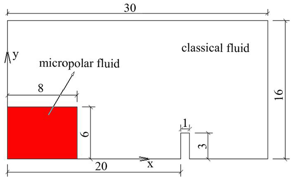
Configuration of dam break (cm).

Divide computation domain by quadrilaterals with an element size of 2 mm, set the surrounding boundary condition as the wall with no-slip, time step is set to 0.001 s, and total calculation time is 0.8 s. The characteristic results are shown as follows.

It can be seen from Table 2 that micropolar parameters have little effect on the pressure and velocity of fluids. The main reason is that the microstructure considered in the model is small, so the influence on macroscopic features is not obvious. However, a certain law can still be seen from the table. As microrotation viscosity decreases, velocity gradually tends to the values calculated under classical fluids, which is consistent with the conclusion in aforementioned examples. It is interesting to notice that the increase in negative pressure eventually exceeds the value obtained by classical fluids, which may be related to the existence of the obstacle. Besides, the microrotation velocity changes significantly exceed the magnitude of 10³ with micropolar viscosity varied from ${\mu }_r=6.69\times {10}^{-4}\mathrm{Pa}·\mathrm{s}$ and ${\mathrm{c}}_{\mathrm{a}}+c_d=0.16\times {10}^{-7}\mathrm{N}·\mathrm{s}$ to ${\mu }_r=1.01\times {10}^{-5}\mathrm{Pa}·\mathrm{s}$ and ${\mathrm{c}}_{\mathrm{a}}+c_d=0.26\times {10}^{-6}\mathrm{N}·\mathrm{s}$ , that is, its absolute value decreases remarkably with the increase in angular viscosity and the decrease in microrotation viscosity.

Table 2.

Physical quantity magnitude at different conditions.

${\mu }_r/c_a+c_d$	variables	0/0	6.69 × 10−4/0.16 × 10−7	6.69 × 10−4/0.64 × 10−7	6.69 × 10−4/0.26 × 10−6	2.51 × 10−4/0.26 × 10−6	1.11 × 10−4/0.26 × 10−6	1.01 × 10−5/0.26 × 10−6
Pressure (Pa)	Maximum	218.91	200.61	201.38	201.59	212.33	216.19	218.03
	Average	102.38	102.15	102.11	102.09	102.09	102.25	101.81
	Minimum	−22.72	−22.31	−22.42	−22.45	−22.93	−22.95	−23.24
Velocity (m/s)	Maximum	0.6410	0.6392	0.6397	0.6398	0.6407	0.6409	0.6410
	Average	0.4785	0.4678	0.4682	0.4683	0.4748	0.4769	0.4784
	Minimum	0.2715	0.2518	0.2522	0.2523	0.2643	0.2683	0.2712
Microrotation	Maximum	–	−9.480	−2.666	−0.719	−0.006	−0.001	0.0002
velocity (s−1)	Average	–	−10.62	−2.967	−0.795	−0.062	−0.018	−0.002
	Minimum	–	−11.83	−3.279	−0.874	−0.265	−0.088	−0.008

Annotation: Data are statistical values taken from the moment $t=0.3s$ , the position $x=19.5\mathrm{cm}$ in front of the obstacle, and the height in the range of $h=0~3\mathrm{cm}$ .

Figure 13 presents the comparison of dam break behavior at different moments between classical fluids and micropolar fluids with ${\mu }_r=6.69\times {10}^{-4}\mathrm{Pa}·\mathrm{s}$ and $c_a+c_d=0.16\times {10}^{-7}\mathrm{N}·\mathrm{s}$ , which (a) represents the dam break pattern under classical fluids and (b) represents the pattern under micropolar fluids. Due to the existence of the obstacle, the kinetic energy of fluids will be converted into potential energy, and when kinetic energy is reduced to the minimum, it will collapse downward and chaotic state appears. But as the scale of microstructures considered is very small, the dynamic characteristics different from the classical fluid are not significant, ²⁸ so the differences only appear after the collapse around the domains I and II.

Figure 13.

Hydrodynamic behaviors at different times.

Figure 14 shows the influence of different micropolar parameters on the variation of dam break behavior. It can be seen that the influence of micropolar parameters is only obvious at the place where large deformation occurs due to the small scale of microstructure considered. However, according to the analysis of above examples, with the increase in microrotation viscosity and angular viscosity, the non-Newtonian characteristics of micropolar fluids will become more and more obvious, that is, the motion of fluids will be gentler as shown in Figure 14(a) with the minimum of maximum velocity 0.6392 m/s.

Figure 14.

The effect of micropolar parameters on hydrodynamic behavior: (a) ${\mu }_r=6.69\times {10}^{-4}$ and $c_a+c_d=0.16\times {10}^{-7}$ , (b) ${\mu }_r=2.51\times {10}^{-4}$ and $c_a+c_d=0.26\times {10}^{-6}$ , (c) ${\mu }_r=6.69\times {10}^{-4}$ and $c_a+c_d=0.64\times {10}^{-7}$ , (d) ${\mu }_r=1.11\times {10}^{-4}$ and $c_a+c_d=0.26\times {10}^{-6}$ , (e) ${\mu }_r=6.69\times {10}^{-4}$ and $c_a+c_d=0.26\times {10}^{-6}$ , and (f) ${\mu }_r=1.01\times {10}^{-5}$ and $c_a+c_d=0.26\times {10}^{-6}$ .

Conclusion

In this article, UDF was adopted to calculate the solution of micropolar fluid equations through the FLUENT software. The impact of microrotation viscosity and angular viscosity on pressure, translational velocity, and microrotation velocity is investigated and discussed in detail.

With the analytical solution of Poiseuille flow provided by MATLAB, it confirmed that the UDF program of micropolar fluid model is correct. And it is convenient and efficient to implement the calculation of the other physical models, for example, micropolar fluids, through the UDF in FLUENT.

The study revealed that the increase in angular viscosity will hinder microrotation velocity, and translational velocity is positively correlated with microrotation viscosity. By comparison, the hydrodynamic behaviors of micropolar fluids will gradually approach to those of classical fluids with the decrease in microrotation viscosity and angular viscosity.

The main work is to fulfill the solution of micropolar fluid equations by UDF and to discuss the influence of micropolar parameters on hydrodynamic behaviors. But the relationship between the concentration of additives and the micropolar parameters is not investigated; also the coupling of micropolar fluids with solid particles will be a research focus in the future.