
Abstract
Ensemble local mean decomposition has been gradually introduced into mechanical vibration signal processing due to its excellent performance in electroencephalogram signal analysis. However, an unsatisfactory problem is that ensemble local mean decomposition cannot effectively process vibration signals of complex mechanical system due to the constraints of moving average. The process of moving average is time-consuming and inaccurate in complex signal analysis. Therefore, an improved ensemble local mean decomposition method called C-ELMD with modified envelope algorithm based on cubic trigonometric cardinal spline interpolation is proposed in this article. First, the shortcomings in sifting process of ensemble local mean decomposition is discussed and, furthermore, advantages and disadvantages of the common interpolation methods adopted to improve ensemble local mean decomposition are compared. Then, cubic trigonometric cardinal spline interpolation is employed to construct the local mean and envelope curves in a more precise way. In addition, the influence of shape-controlling parameter on envelope estimation accuracy in cubic trigonometric cardinal spline interpolation is also discussed in detail to select an optimal shape-controlling parameter. The effectiveness of cubic trigonometric cardinal spline interpolation for improving the accuracy of ensemble local mean decomposition is demonstrated using a synthetic signal. Finally, the proposed cubic trigonometric cardinal spline interpolation is tested to be effective in gear and bearing fault detection and diagnosis.
Keywords
Introduction
With the development of industrial technology, rotating machinery in modern mechanical systems is becoming more and more complex to satisfy the increasing application requirement. 1 However, the rotating machinery is vulnerable to failures due to its structural complexity, especially under harsh operating conditions. To improve system reliability and reduce accidental downtime, rotating machinery fault diagnosis has been widely adopted in modern industrial applications. Over the past decade, numerous fault diagnosis techniques such as expert systems, fuzzy logic, machine learning algorithm, and model-based methods have been introduced for rotating machinery fault diagnosis.2–5 Fault diagnosis is described as the process to determine whether the system is operating normally or not and to find incipient failures and their causes based on operational information obtained from the mechanical equipment.6,7 Fault feature extraction which can be accomplished through a vibration signal process is the key step of fault diagnosis. Common signal processing methods can be generally categorized into time-domain signal analysis methods, frequency domain signal analysis methods, and time-frequency domain signal synthetic analysis methods.3–6 However, fault signals of rotating machinery with multistage transmission usually appear nonlinear and non-stationary properties, which can be diagnosed effectively by only utilizing time-frequency synthetic analysis methods. Furthermore, the complex transmission paths from fault to sensors also makes the original signal contain a lot of interference information which further increase the difficulty of feature extraction.8,9
To overcome the above barriers, several advanced time-frequency analysis methods, such as singular value decomposition (SVD), wavelet transform (WT), and Hilbert-Huang transform (HHT) have been investigated to extract intrinsic information from non-stationary and nonlinear signals. Jiang et al. 10 used SVD to reduce the background noise in wind turbine signals and integrated SVD and Merlot wavelet for fault feature extraction. Zhao and Jia 11 proposed a reweighted SVD to improve the ability in weak feature identification and applied it for weak feature enhancement. Law et al. 12 improved the computation efficiency of HHT and combined it with wavelet packet decomposition for spindle bearing condition monitoring. Jiang et al. 13 made use of the multiresolution of multiwavelet packet to refine the original signal and combined it with ensemble empirical mean decomposition (EEMD) for multi-fault diagnosis. However, WT cannot effectively deal with the high frequency which contains abundant fault modulation information. Although wavelet packet transform (WPT) overcomes this drawback, the selection of wavelet basis function depends on personal experience when dealing with practical signals which makes WPT non-adaptive.14,15 HHT is an effective adaptive signal processing method which is not subject to the Heisenberg uncertainty principle. It can achieve high resolution simultaneously in time-frequency space. However EMD, as the core of HHT, usually suffers from serious end effects and mode mixing. Wu and Huang 16 proposed EEMD to alleviate mode mixing by using the statistical properties of white noise. Although EEMD can alleviate mode mixing, there are still many deficiencies such as added noise amplitude selection and extremum interpolation.17–21
A relatively new method named local mean decomposition (LMD) was proposed by Smith 22 for electroencephalogram signal analysis. LMD uses a natural and a priori way to decompose the non-stationary/nonlinear signal into a series of physically meaningful product functions (PFs). Compared with EMD, LMD decomposes signals into fewer levels and retains more useful information in the decomposed result, which means that this method may have better performance in fault detection.22,23 Accordingly, it has been introduced in rotating machinery fault diagnosis.23–27 As a new time-frequency method without systematic mathematical proof, LMD still has some deficiencies such as end effects, mode mixing, and envelope estimation. By extending the waveform based on spectral coherence, Guo et al. 28 eliminated the decomposition errors caused by end effects. To reduce mode mixing, ensemble local mean decomposition (ELMD) was proposed by Cheng, which presented better performance than EEMD in fault diagnosis.29,30 Subsequently, Zhang et al. 31 optimized the parameters of ELMD to further improve the performance of ELMD. However, the essence of ELMD is repetitive iterations of LMD, which does not fundamentally increase the accuracy of calculation results. In ELMD, moving average (MA) constructs the local mean and envelope estimation by smoothing the local means and local magnitudes step by step. After smoothing, interpolation line segment turns into a smooth curve, but this process can only ensure that the calculation result is a smooth continuous curve without any discontinuity. It is difficult to prove the existence of derivative of interpolation curve mathematically, let alone continuous first derivative. In general, the higher the interpolation number of polynomial, the more accurate the interpolation curves, which means that interpolation functions with continuous high-order derivatives are helpful to improve the performance of ELMD decomposition. And the gradual smoothing of MA is an inefficient progress. Therefore, a variety of high-order interpolation algorithms, such as piecewise linear interpolation, cubic spline interpolation, and rational spline interpolation, have been introduced to calculate the local mean and envelope estimation curves in a more accurate way.32–35 Comparison of these interpolation methods is critically reviewed highlighting their advantages and disadvantages. Piecewise linear interpolation has good uniform convergence, simple construction, and high numerical accuracy. However the interpolation curve is not smooth at the connection point and its accuracy depends on the density of interpolation nodes which means the smaller the interpolation interval, the higher the accuracy of calculation. Therefore, it is difficult to obtain accurate calculation results with less computation. Cubic spline interpolation is a common lower-order piecewise interpolation method with relatively simple calculation process, and it can use lower-order piecewise polynomials to express high-order smooth curves. Although cubic spline interpolation has high computation accuracy, the interpolation curves may exhibit numerical oscillation (Runge phenomenon) which will lead to overshoot/undershoot problems. Rational spline interpolation is a typical nonlinear interpolation method which is more accurate than polynomial interpolation. The curves generated by rational spline interpolation are smoother than those of polynomial interpolation. What’s more, rational spline interpolation can improve the mathematical properties of interpolation curves by selecting appropriate shape parameters to overcome numerical oscillation. But rational spline interpolation utilizes rational expressions to construct the spline which is difficult to select the tension parameter and the computational cost is enormous.36,37
Therefore, a novel interpolation algorithm called cubic trigonometric cardinal spline interpolation (CTCSI) is introduced to construct the local mean and envelope estimation functions in this article. After obtaining the midpoints of the local extreme points, the corresponding interpolation functions can be constructed utilizing CTCSI. The improved ELMD method based on CTCSI is called C-ELMD. The remainder of this article is organized as follows. A review of ELMD and CTCSI is presented in section “Review of ELMD and CTCSI.” The main steps of the C-ELMD are described in section “Improved ELMD.” Section “C-ELMD for rotating machinery fault diagnosis” introduces the experimental process of rolling bearing and gear and analyzes the results which demonstrate the effectiveness of C-ELMD for rotating machinery fault diagnosis. Finally, a brief summary and the final conclusion are given in section “Discussion and conclusions.”
Review of ELMD and CTCSI
Ensemble local mean decomposition
ELMD is a substantial improvement on LMD to overcome mode mixing. The reason for mode mixing is that the original signal contains intermittent parts with discrete time-scale distributions. Inspired by EEMD, ELMD add Gaussian white noise to the original signal, and utilize the uniform distribution of Gaussian white noise in time-frequency space to alleviate mode mixing. Finally, the Gaussian white noise can be eliminated in the ensemble mean. 13 The process of ELMD is actually utilizing LMD to decompose the noise-added signal repeatedly. Therefore, a clear understanding of the principle of LMD is helpful and necessary to improve ELMD effectively.
LMD is a double-loop iterative process (i.e. an inner loop within the body of an outer one) with interpolation, multiplication, and division algorithm, which realizes signal decomposition by reasonably arranging the order among various algorithms. The function of the inner loop is to extract a single PF from the original signal, and the function of the outer loop is to decompose the original signal completely, so that components with different characteristics are allocated to different PF. Given
Identify the local extremums


where
Extending the local mean and local magnitude points obtained in Step 1 with straight line to form the corresponding line segment. These segments are then smoothed utilizing MA to generate the smoothly continuous local mean function
Subtract local mean function


where
If

where

Then the first envelope function and PF can be derived as follows


where
Finally, after a certain number of cycles

Cubic trigonometric cardinal spline interpolation
As described in section “Ensemble local mean decomposition,” the accuracy of local mean function
Compared with the interpolation process of MA, four points are utilized for each interpolation process of CTCSI which can greatly improve the calculation accuracy of interpolation function. The main idea of CTCSI is to interpolate the value of related points as the coefficients of the basis function and select appreciate basis function so that the interpolation curve can satisfy C1 continuous. Following are the definitions of the basis functions. 38
Definition 1
Suppose
where
For any given value for

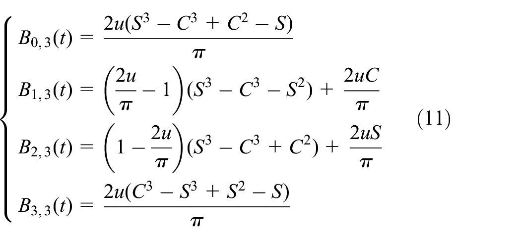
These properties of the basis function can guarantee the continuity of the interpolation curve. What’s more, we can obtain different basis function curves by adjusting the value of u, which means that the basis functions have good flexibility. Therefore, u is called shape-controlling parameter. The specific basis functions Bj,3(t) corresponding to

Basis functions of the CTCSI: (a) u = 0.5 and (b) u = 1.0.
Definition 2
We define qi (i = 1,2,…,)) as a series of discrete points. For any set of four ordinal control points, qi–1, qi, qi + 1, qi + 2, the parameter curve segments can be defined as follows

where
For any given four successive points qi–1, qi, qi + 1, qi + 2, CTCSI construct the interpolation curve between qi and qi + 1 , while the values of points qi–1 and qi + 2 are used to control slopes of the interpolation curve. Because there is a shape-controlling parameter, u, in the basis function, different spline curves can be obtained by changing the value of u. Furthermore, it has been proven that cubic trigonometric cardinal interpolation is C1 continuous which means the first derivative is smooth and continuous. 38 The envelopes constructed by CTCSI with shape-controlling parameter u values of 0, 0.2, 0.5, 0.8, and 1.2 are shown in Figure 2. The shapes of the envelopes progressively change as u varying. As can be seen from Figure 2, the spline curve is a convex interpolation spline curve when the value is small. And it becomes a ring buckle interpolation spline with two emphases when the value is too large (such as u = 1.2 in Figure 2), which is time-consuming and useless. Hence, the value of controlling parameter u should range from 0.3 to 0.7 to guarantee calculation efficiency and calculation accuracy. Research by Ping inspired us to set u = 0.5, which guarantees the best continuity of the spline curve. 38 The analysis of Figure 2 also confirms this; thus, we will set u = 0.5 for the rest of this article.

A range of values u combined with CTCSI to obtain upper and lower envelopes.
Improved ELMD
As mentioned above, the main process of ELMD is to decompose the noisy signal using LMD repeatedly. The decomposition performance of LMD is greatly affected by the accuracy of local mean and envelope estimation function. However, current smoothing algorithms, such as MA, cannot meet the requirements of computational accuracy under complex conditions. Therefore, a new interpolation method called CTCSI is adopted to construct the interpolation curves more precisely. The main procedures of envelope curve fitting process are given as follows:
Identify the local extremums of a signal and construct the upper envelope function
Calculate the local mean function


From the perspective of algorithm execution sequence, LMD is a double-loop iterative process. C-ELMD achieves accurate decomposition of signals through multiple iterations of LMD with improved interpolation algorithm. Thus, C-ELMD is essentially a three-loop iterative process. To understand this process easily, we can also regard C-ELMD as a double-loop iterative process, with the inner loop being the improved LMD and the outer loop being the process of introduction and elimination of the noise signal. The above are two descriptions of C-ELMD based on algorithm principle and execution process. Furthermore, it will be easier to understand the whole process of C-ELMD, if we treat the sequential outer loop as independent parallel structures. And the corresponding flowchart of C-ELMD is illustrated in Figure 3.

Flowchart of C-ELMD method.
C-ELMD for rotating machinery fault diagnosis
In this section, we test the performance of C-ELMD in fault diagnosis of rotating machinery. Rolling bearings and gears are important components to transmit power and motion in rotating machinery, and the failure of these components may lead to a breakdown of the whole system. Therefore, a simulation signal with modulation characteristics and two experimental signals collected from test rig with bearing and gear local fault are used to evaluate the effectiveness of C-ELMD in rotating machinery fault diagnosis. Comparison results show that the proposed C-ELMD outperforms existing ELMD and RS-ELMD.
Performance test using a simulation signal
Signals from rotating machinery with faults, especially local faults, usually present amplitude modulation and frequency modulation when the fault occurs in the gears or roller bearings.39–41 Therefore, a multi-component amplitude modulation simulated signal

where randn(n,1) is the noise signal; α is the signal-to-noise ratio which is set to be 0.16 in this article; and length(x1) is the length of x1(t).
The simulated signal consists of an amplitude-modulated signal, a sinusoidal harmonic signal, and a white Gaussian noise. Its spectrum and components are shown in Figure 4. The signal time duration is 0.5 s and the sampling frequency is 5000 Hz.

Simulated signal, its spectrum, and components: (a) Waveform of the simulated signal; (b) FFT spectrum of the simulated signal; (c) Components of the simulated signal.
To test the performance of the proposed C-ELMD, comparisons are conducted with ELMD and an improved ELMD based on rational Hermite interpolation (RS-ELMD). Orthogonality index (OI) and root mean square error (RMSE) are used as evaluation indicators. The reasons for selecting OI and RMSE are described as follows:
The concept of orthogonality comes from geometry to describe the perpendicular relationship between two lines. In terms of signal processing, orthogonality can be used to describe the correlation between two signals. Although different PF is not strictly orthogonal, there should be little or no similarity between them. This index can quantitatively describe the quality of decomposition results from the perspective of correlation. If the value of OI is large, there are many identical parts between different PF which means the decomposition result is poor and there is likely to be mode mixing; on the contrary, if the value of OI is small, that means the decomposition is good and effective. The expression of OI is given as follows

where NPF is the number of PFs, N is the length of the PF, PFik(t) and PFjk(t) are the ith and jth PF at the kth sifting step, respectively,
The use of RMSE is very common in statistical analysis and its physical meaning is to measure the difference between two datasets. It compares a predicted value and an observed or true value and quantifies how different two sets of values are. The smaller an RMSE value, the closer predicted and observed values are. Therefore RMSE can be used as an effective index for quantitative analysis of C-ELMD decomposition accuracy. The smaller of this index value, the closer PFs and corresponding sub-components of the original signal are, indicating the higher the decomposition accuracy is. The definition of RMSE is described as follows

where s(t) is defined sub-component of the original signal corresponding to the PF(t).
The simulated signal is decomposed using ELMD, RS-ELMD, and C-ELMD, respectively. The noise amplitude is set as A = 0.2 and the ensemble number is set as M = 100 for comparison. 31 The decomposition results of these three methods are presented in Figure 5. It shows that all three methods can successfully decompose x1(t) and x2(t) from the simulated signal x(t). The PF1(t) and PF2(t) components correspond to x1(t) and x2(t) of the original signal, respectively. However, the PF2(t) obtained by ELMD and RS-ELMD have mode mixing problems to a certain extent. Furthermore, the results of ELMD show a mode mixing phenomenon more serious than that of RS-ELMD. However, mode mixing can hardly be observed in PF2(t) obtained by C-ELMD, which means that C-ELMD has obvious advantages in decomposition effectiveness and precision compared with ELMD and RS-ELMD. As can be seen from Table 1, the values of OI and RMSE obtained by C-ELMD are also smaller than those obtained by ELMD and RS-ELMD. This indicates that C-ELMD achieves better decomposition performance than the other two methods.

Decomposition result of the simulated signal utilizing ELMD, RS-ELMD, and C-ELMD, respectively: (a) ELMD, (b) RS-ELMD, and (c) C-ELMD.
RMSE and OI indicators of ELMD, RS-ELMD, and C-ELMD.

ELMD: ensemble local mean decomposition; RS-ELMD: rational Hermite interpolation; C-ELMD: improved ELMD method based on CTCSI; RMSE: root mean square error; OI: orthogonality index.
Experimental validation for bearing fault diagnosis
In this experimental case, the applicability of C-ELMD in bearing fault diagnosis is tested using the experimental signals of a roller bearing with local defects on the outer ring. The bearing data were obtained from Case Western Reserve University (CWRU) Bearing Data Center. 42 This experimental dataset has been cited by many researchers as a benchmark for bearing fault diagnostics. The bearing test platform is mainly composed of a 2-hp reliance electric motor, a torque transducer, a dynamometer, and control electronics (not shown) as shown in Figure 6. There are two bearings in the test system, one supporting the drive spindle and the other supporting the fan spindle. Three types of faults with different severity levels have been manually made on test bearings utilizing an electrical-discharge machining. Detailed information about the test platform including bearing specifications, fault frequencies, related experimental parameters, and vibration data files can be found on the CWRU website. 42 The vibration signals collected on the drive-end bearing with pitting damage is used to test our proposed method. The fault is located in the 3 o’clock position on the outer race and the corresponding fault diameter is 21 mils. The vibration signal was measured at a motor speed of 1797 r/min (fr = 28.5 Hz) and sampling frequency of 48 kHz. The fault characteristic frequency can be determined by multiplying the rotating frequency by the outer ring coefficient of the drive-end bearing. The coefficients of the bearing are listed in Table 2, from which the fault characteristic frequency feq could be calculated as follows

where fr is the rotating frequency of the motor, and Co is the outer ring coefficient.

Bearing test rig of CWRU.
Coefficients of the drive-end bearing.

A vibration signal of the drive-end bearing and its spectrum are shown in Figure 7. Figure 7 shows that although the vibration signal presents clearly periodicity, we can only find rotating frequency of the drive-end bearing. This information alone is insufficient to provide evidence for fault diagnosis. Further processing and advanced signal processing technology are needed to extract the fault information which is totally submerged by noise and other interference.

Experimental bearing vibration signal and its spectrum: (a) time-domain waveform and (b) FFT spectrum of bearing vibration signal.
The above preliminary analysis suggests that the existent of interference information is bad for fault diagnosis. Therefore, it is promising to use C-ELMD to decompose the original signal into multiple independent components, then, fault information and interference information are separated, which can reduce the influence of interference information. The bearing vibration signal decomposition result obtained by means of C-ELMD is shown in Figure 8(c). For comparison, ELMD and RS-ELMD are also applied to the same bearing signal with the same conditions and the decomposition results are shown in Figure 8(a) and (b), respectively. As shown in Figure 8, PF1(t), similar to the original signal, presents clearly periodicity; PF2(t) shows a weak periodicity, and the rest of the decomposition results vibrate irregularly. Time-domain waveform of the results obtained by these three methods show little difference. However, the evaluation indicators (RMSI and OI) show that three methods are different (see Table 3). From the comparison of the evaluation indicators for the above three methods, we can draw the following conclusion: the performance of RS-ELMD in this case is better than ELMD, and C-ELMD is far better than ELMD and RS-ELMD. But this information is still insufficient for fault diagnosis. According to the above analysis, fault information is mainly distributed is PF1(t), hence, it is selected for further analysis.

Decomposition result of the bearing vibration signal by means of ELMD, RS-ELMD, and C-ELMD respectively: (a) ELMD, (b) RS-ELMD, and (c) C-ELMD.
Comparison of the evaluation indicators of bearing data for ELMD, RS-ELMD, and C-ELMD.
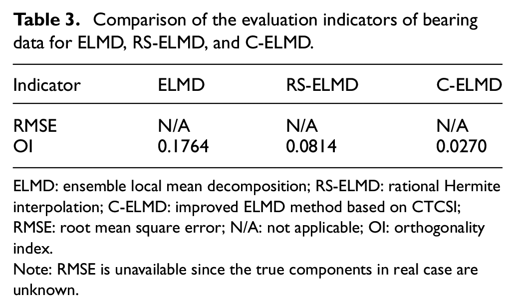
ELMD: ensemble local mean decomposition; RS-ELMD: rational Hermite interpolation; C-ELMD: improved ELMD method based on CTCSI; RMSE: root mean square error; N/A: not applicable; OI: orthogonality index.
Note: RMSE is unavailable since the true components in real case are unknown.
The time-domain waveform of PF1(t) and its envelope spectrum for those three methods are shown in Figures 9–11, respectively. The fault characteristic frequency feq and its second harmonic frequency 2feq in Figure 9 is almost unrecognizable. The fault characteristic frequency feq, and its second harmonic frequency 2feq, and third harmonic frequency 3feq can be seen from Figure 10. In Figure 11, the fault characteristic frequency feq, its second harmonic frequency 2feq, third harmonic frequency 3feq and side-band frequency can be clearly identified. Combine the above analysis results, C-ELMD is more effective in bearing fault diagnosis than ELMD and RS-ELMD.

Spectrum analysis of ELMD: (a) time-domain waveform of PF1(t); (b) envelope spectrum of PF1(t).

Spectrum analysis of RS-ELMD: (a) time-domain waveform of PF1(t); (b) envelope spectrum of PF1(t)
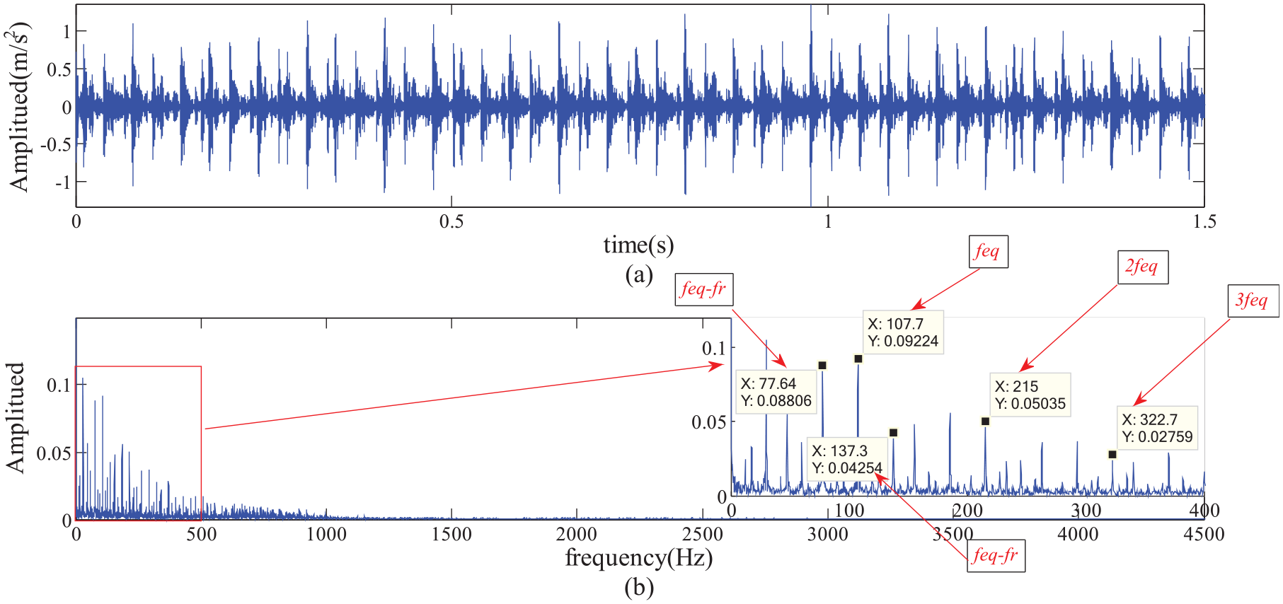
Spectrum analysis of C-ELMD: (a) time-domain waveform of PF1(t); (b) envelope spectrum of PF1(t).
Experimental validation for gear fault diagnosis
In many existing studies, the signals are collected from laboratory research gearboxes which only have one or two pairs of gears. Laboratory gearboxes may not have oil lubrication system, connectors, fasteners, and support components found in practical engineering gearboxes for economy and efficiency purpose. Hence, vibration signals collected from these laboratory-simplified gearboxes may not good enough to reflect the health conditions of practical engineering gearboxes. Therefore, a scaled wind turbine gearbox was constructed in our study to test the proposed method.
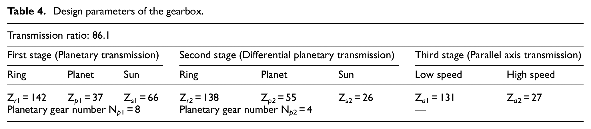
The gear test platform is illustrated in Figure 12. The system included two gearboxes with the same design parameters, a 3-hp AC, and a magnetic brake. A structural sketch of the test rig and a schematic diagram of the wind turbine gearbox are displayed in Figure 13. To simulate the practical working situation, one of the gearboxes connected to the motor works as a reduction gearbox to convert the high-speed output of the motor into low-speed output. The other one runs as the experimental subject. The design parameters of the gearbox are listed in Table 4.

Test rig of the wind turbine gearbox.
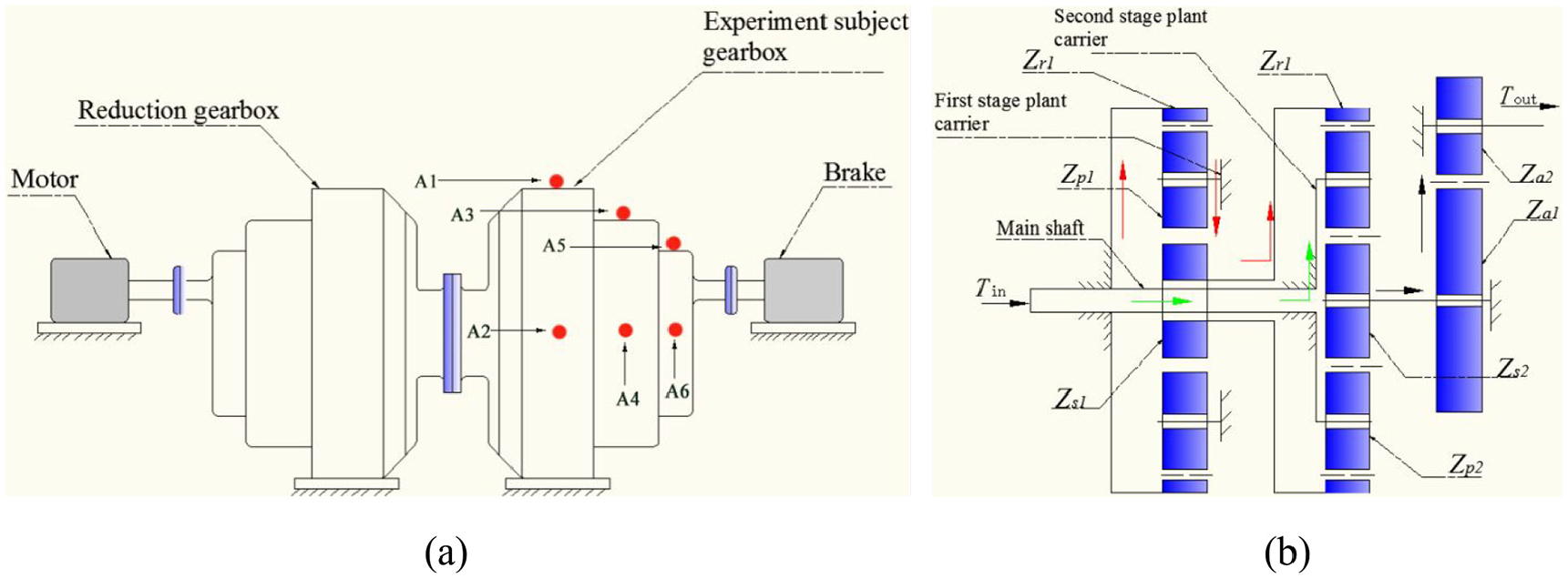
Diagram of gear test rig and gearbox: (a) Structural diagram of the gear test rig; (b) Schematic diagram of the gearbox.
Design parameters of the gearbox.
The third-stage high-speed gear, Za2, with pitting fault, was simulated in the experimental system. A photograph of the faulty gear and a schematic of the pitting damage are shown in Figure 14. The vibration signal is measured at a motor speed of 1450 r/min (fr = 24.17 Hz) and the sampling frequency is 6.4 kHz. Accelerometers are installed on the gearbox housing, as shown in Figure 13(a). The specific location is optimized according to the shortest transfer path principle. According to the configuration and design parameters of the gearbox, the fault characteristic frequency feq and the third-stage mesh frequency fh can be calculated as follows


Fault gear and its pitting schematic: (a) Fault gear; (b) Schematic of pitting damage.
Vibration signal of the faulty gear and its spectrum are illustrated in Figure 15. In Figure 15(a), it is difficult to see any periodic characteristic signal, which means that background noise and other interference components account for a large proportion of the original signal. Even though the frequency components in Figure 15(b) are clear with little interference, there is no frequency component associated with gear fault. This indicates that vibration signals observed in practical engineering are more complex than those observed in the laboratory due to complex mechanical systems.
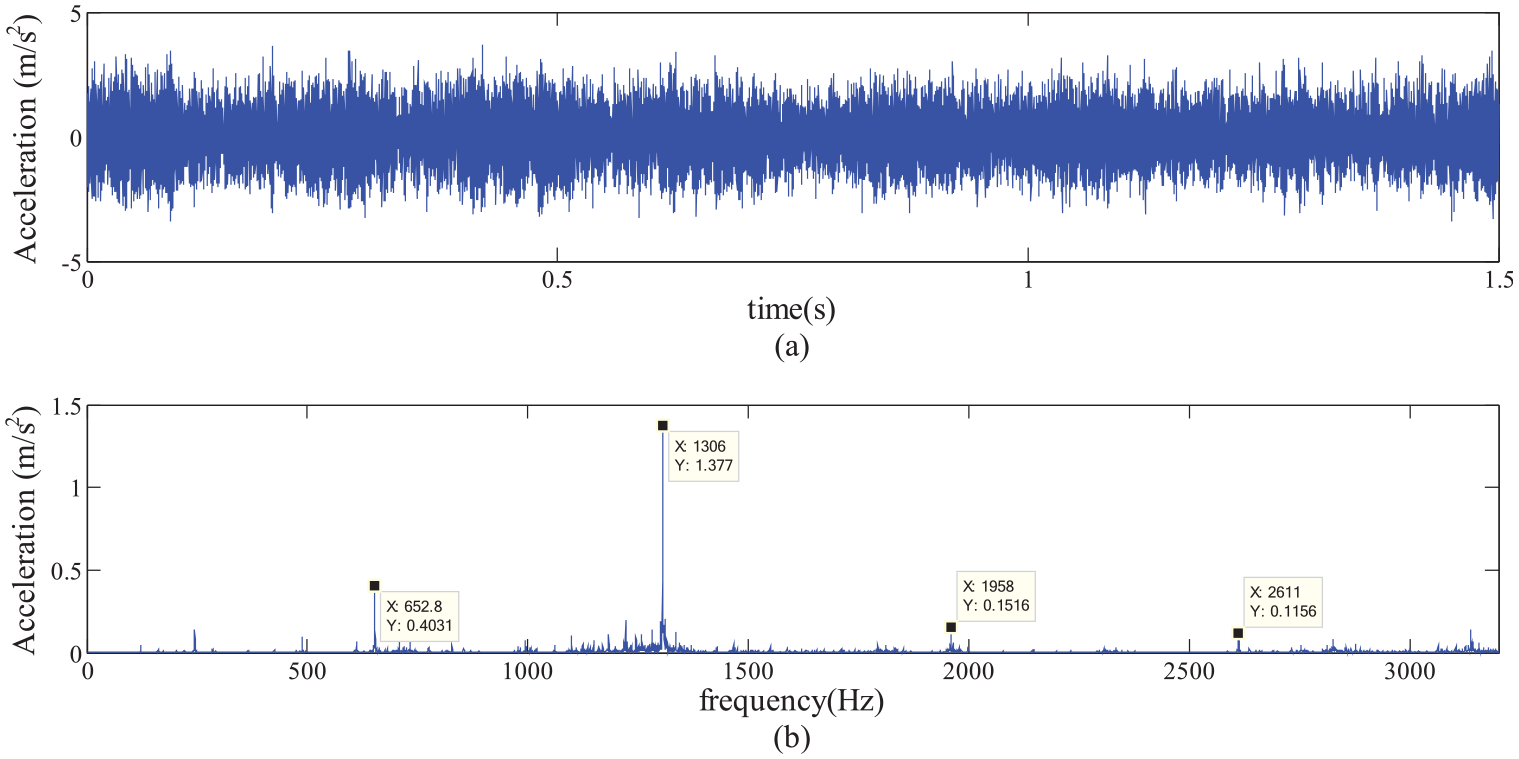
Experimental gear vibration signal and its spectrum: (a) Time-domain waveform; (b) FFT spectrum of gear vibration signal.
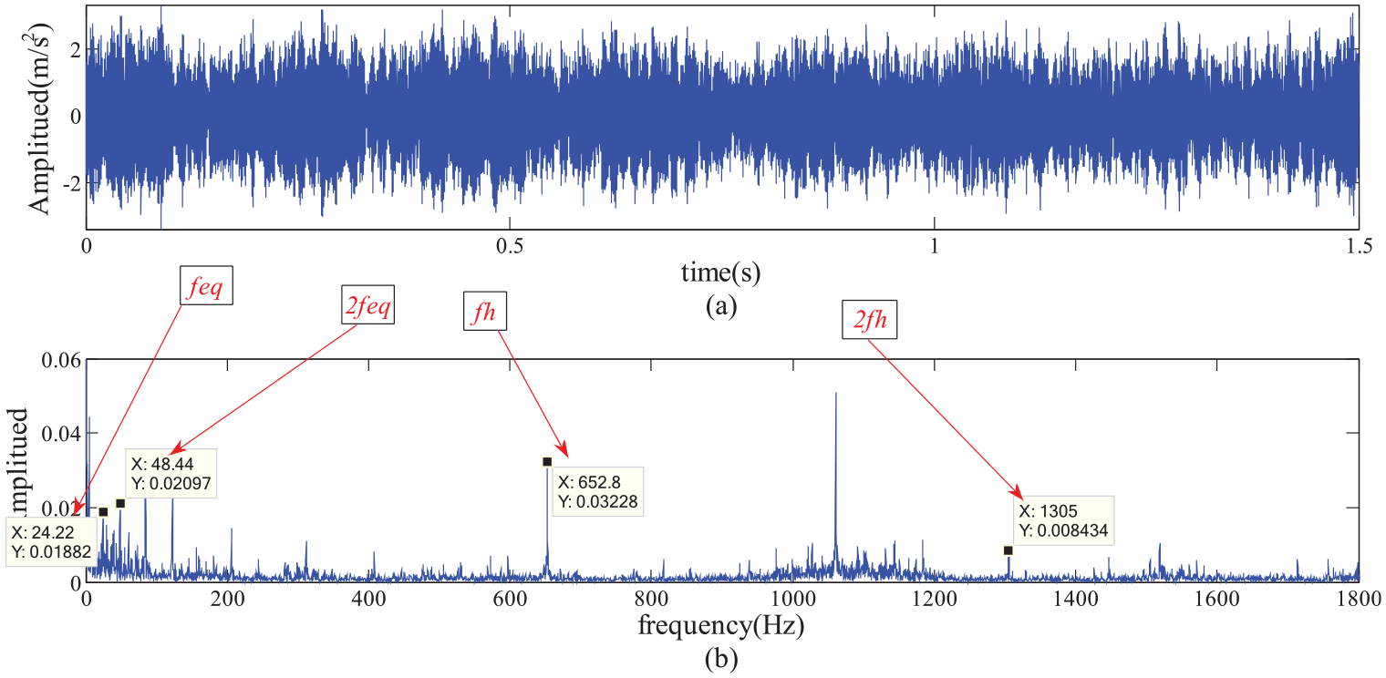
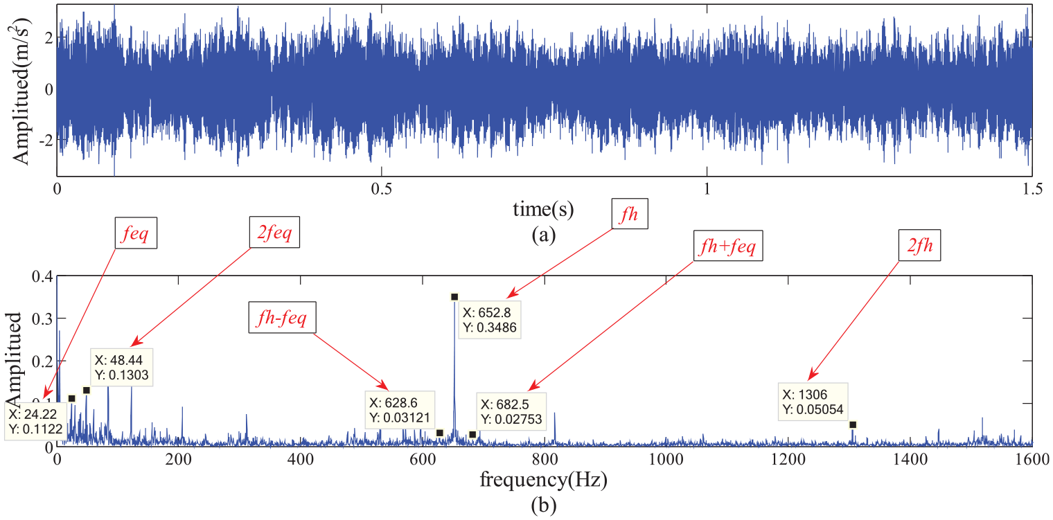
ELMD, RS-ELMD, and C-ELMD are applied for fault information extraction and the decomposition results of the faulty gear vibration signal are shown in Figure 16. The envelope spectrum analysis is applied afterward. The waveform of PF1(t) obtained by those three methods and its envelope spectrum are presented in Figures 17–19, respectively. Adopting the same strategy, the waveform of decomposition results and its evaluation indicators are used for comparison. Based on the comparison of waveform and evaluation indicators, we can get conclusions similar to section “Experimental validation for bearing fault diagnosis” that the performance of RS-ELMD is better than ELMD, and C-ELMD is far better than ELMD and RS-ELMD. Then, the spectrum is compared and analyzed. Although there is still no obvious periodic vibrational characteristic, Figure 19(a) and (b) has sufficient information to diagnose the gear fault. In Figure 19(b), we can clearly see the fault frequency component feq, its second harmonic frequency 2feq and third harmonic frequency 3feq, and side-band frequencies which indicate that the third-stage high-speed gear of the gearbox is working with fault. However, only the fault frequency component feq, its second harmonic frequency 2feq, and the meshing frequency fh can be obtained in Figure 17(b) and this information is insufficient for fault diagnosis. Figure 18(b) contains more information compared with Figure 17(b), such as the fault frequency component feq, its second harmonic frequency 2feq, mesh frequency fh and second harmonic frequency 2fh, and the side-band frequencies loading in fh. Fault diagnosis decision can be made based on the information in Figure 18(b), but errors may occur or extensive experience is required. The analysis results in this case study demonstrate the effectiveness of the C-ELMD for gear fault diagnosis. The evaluation indicators of gear data are listed in Table 5.
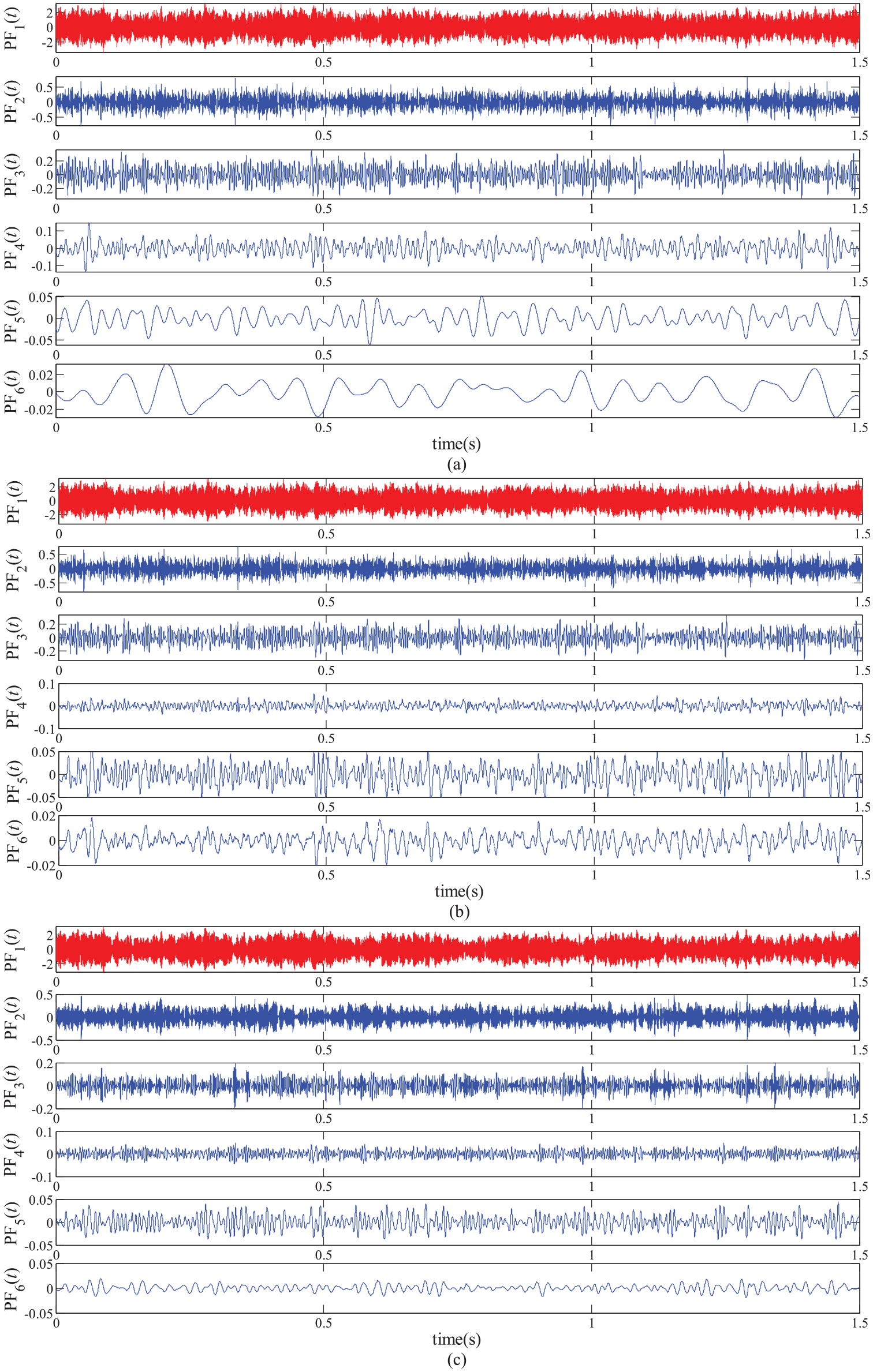
Decomposition result of the gear vibration signal by means of ELMD, RS-ELMD, and C-ELMD respectively: (a) ELMD, (b)RS-ELMD, and (c) C-ELMD.
Spectrum analysis of ELMD: (a) time-domain waveform of PF1(t); (b) envelope spectrum of PF1(t).
Spectrum analysis of RS-ELMD: (a) time-domain waveform of PF1(t); (b) envelope spectrum of PF1(t).

Spectrum analysis of C-ELMD: (a) time-domain waveform of PF1(t); (b) envelope spectrum of PF1(t).
Comparison of the evaluation indicators of gear data for ELMD, RS-ELMD, and C-ELMD.
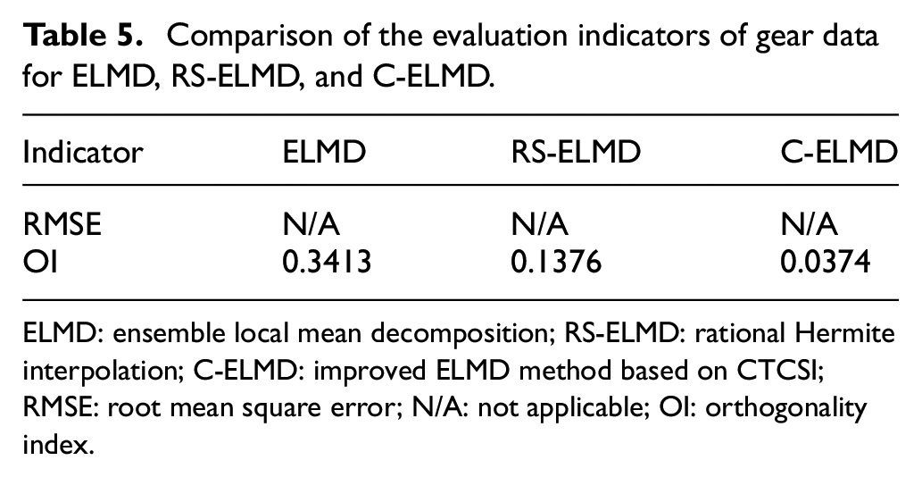
ELMD: ensemble local mean decomposition; RS-ELMD: rational Hermite interpolation; C-ELMD: improved ELMD method based on CTCSI; RMSE: root mean square error; N/A: not applicable; OI: orthogonality index.
Discussion and conclusion
This article originated from the research on the application and improvement of ELMD in rotating machinery fault diagnosis. Based on the comprehensive analysis of vibration signal characteristics, CTCSI is proposed to replace the original interpolation algorithm MA to improve the performance of ELMD. The quantitative evaluation indexes of the synthetic signal show that compared with ELMD and RS-ELMD, C-ELMD has significant advantages in reducing mode mixing and improving decomposition accuracy. In consideration of the complexity of vibration signals encountered in practical engineering scenarios, vibration signal obtained from a CWCRU bearing test system and a scale wind turbine gearbox was used to verify the effectiveness of C-ELMD. The fault characteristic frequency, second harmonic frequency, and corresponding side-band frequencies can be seen clearly from the analysis results of C-ELMD, which validates its effectiveness for rotating machinery fault diagnosis.
But what needs to be pointed out is that the improvement of ELMD interpolation algorithm in this article and previous articles are based on the signal characteristics of their specific applications. As shown in the analysis results of section “Experimental validation for gear fault diagnosis, although the fault characteristic frequency of a gear signal can be found in the spectrum analysis of PF1(t) obtained by C-ELMD, there is no obvious periodic vibrational characteristic, which means PF1(t) contains other interference terms. That is to say, there are still mode mixing in the decomposition result of C-ELMD in this case. The proposed method still has a place for further improvement. In future, the authors will also investigate theoretical properties of the proposed interpolation algorithm and give theoretical explanation of their effect on the decomposition accuracy of ELMD.
Footnotes
Acknowledgements
We appreciate the reviewers and editors for their valuable comments.
Handling Editor: James Baldwin
Declaration of conflicting interests
The author(s) declared no potential conflicts of interest with respect to the research, authorship, and/or publication of this article.
Funding
The author(s) disclosed receipt of the following financial support for the research, authorship, and/or publication of this article: This research is supported by the Key Program for International S&T Cooperation Projects of China (Grant No. 2015DFA71400), Natural Science Foundation of China (Grant No. 51975535).