Study on bifurcation characteristics of multi-clearance bending torsional coupling gear transmission based on EHL

Abstract

In order to study the influence of tooth surface friction on the non-linear bifurcation characteristics of multi-clearance gear drive system, a 6 degree-of-freedom bending torsional coupled vibration model was established. The time-varying mesh stiffness, backlash, support clearance and damping were considered comprehensively in this non-linear vibration model. Loaded tooth contact analysis was used to calculate the time-varying mesh stiffness. Based on the elasto-hydrodynamic lubrication, the time-varying friction coefficient was calculated. Runge–Kutta numerical method was used to solve the dimensionless dynamic differential equation. Using phase diagram, Poincaré diagram, time history diagram, and spectrum diagram, the influence of tooth surface friction on bifurcation characteristics was studied. The results show that the system undergoes a change from 1-periodic motion, multi-periodic motion, to chaotic motion through bifurcation and catastrophe when the speed changes independently. When the friction coefficient of tooth surface changes from 0, 0.05 to 0.09, the chaotic motion of the system is suppressed. Similarly, with the increase in tooth friction, the chaotic motion characteristics are suppressed. Tooth surface friction is the main factor affecting chaotic motion. With the increase in friction coefficient of tooth surface, the chaos characteristic does not change obviously and the vibration amplitude decreases slightly.

Introduction

Tooth surface friction is one of the key factors that affect the vibration and noise of the gear transmission system. In order to clarify the non-linear dynamic behavior of the gear transmission system under the real working condition, many scholars have done a lot of work on the research of the non-linear dynamic model of the gear with friction. Azar and Crossley ¹ considered the time-varying mesh stiffness, tooth surface friction, tooth separation, and gear modification and established the differential equation of motion of spur gear transmission system. Rao ² explored the coupling characteristics of friction coefficient and backlash and found that the change in backlash will affect the friction coefficient. Yang and Lin ³ established the differential equations of motion of spur gear transmission system including involute profile, energy loss, time-varying mesh stiffness, material elastic modulus, backlash and tooth surface friction. Kahraman and Singh ⁴ established a 3-degree-of-freedom (DOF) gear system non-linear model considering the non-linear factors such as support clearance, backlash, and time-varying mesh stiffness. Menon and Krishnamurthy ⁵ established a dynamic model including tooth surface friction and tooth side clearance and applied neural network compensation method to explore its dynamic impact on the transmission system. Velex and Cahouet ⁶ established the finite element model of spur gear and helical gear with friction, based on Coulomb friction theory and finite element theory. Howard et al. ⁷ established the dynamic model of spur gear transmission system with 16 DOFs including the factors affecting the friction of tooth surface. Vaishya and Singh^8–10 established a dynamic model considering friction and simplified the time-varying mesh stiffness to rectangular wave. Wang et al. ¹¹ analyzed the chaos and bifurcation phenomenon of the gear transmission model with 2DOFs including friction. Yuan et al. ¹² studied the application of fractal description in the characterization of engineering surface and wear particles. Lundvall et al. ¹³ used the method of multi-body dynamics to establish a 3-DOF motion differential equation including friction. He et al. ¹⁴ established a multi-DOF dynamic model including friction of tooth surface based on Coulomb friction theory. Liu and Parker ¹⁵ established the coupling vibration mechanical model of a single pair of gear system including friction, stiffness, and damping. Tang et al. ¹⁶ established a single pair of gear transmission system dynamics model considering friction, clearance, stiffness, and other factors. Zhang et al. ¹⁷ established a 6-DOF dynamic model including friction and solved the influence of tooth surface roughness on friction by numerical method. Lu et al.^18,19 use the normal distribution function to describe the random backlash and analyze the dynamic characteristics of single-pair gear transmission system. Wen et al. ²⁰ studied the response of a single-DOF gear system with random backlash under white noise excitation. Wang ²¹ established the dynamic model of herringbone gear including tooth friction and analyzed the influence of tooth friction on chaos and bifurcation of the system. Ma et al. ²² have studied the research progress of the dynamics of the gear transmission system with cracks. Bao et al. ²³ studied the dynamic characteristics of variable pitch external gear system with time-varying friction coefficient. Zhou et al. ²⁴ studied the non-linear dynamic characteristics of the coupling gear rotor bearing system under the internal and external excitation. Lu et al. ²⁵ studied the non-linear vibration characteristics of the gear rotor bearing system. Wang et al. ²⁶ studied the establishment method of time-varying mesh stiffness model of helical gear pair considering axial meshing force. Yin et al. ²⁷ studied the dynamic modeling and analysis of single-stage gear system with tooth impact and friction. Li et al.^28,29 studied the influence of the backlash with fractal characteristics on the dynamic characteristics of the gear bearing system. Chen et al.^30,31 introduced the fractal theory and studied the influence of the gear backlash with fractal characteristics on the dynamic characteristics of single-stage gear system. Shi and Zhao ³² studied the vibration characteristics of the second-stage helical cylindrical gear rotor system and believed that the high-frequency modal frequency of the gear rotor system changed greatly with the rotating speed due to the existence of gyroscopic effect. Zhang et al. ³³ studied the stiffness calculation and influence factor analysis of spur gear pair considering time-varying friction.

From the above studies, some research has been done on the non-linear characteristics of gear transmission systems with considering the friction of the tooth surface. However, in most of these studies, the actual meshing changes in the tooth surface loaded contact process are less considered. Therefore, in order to study the influence of tooth surface friction on the bifurcation characteristics of the system, through considering the time-varying mesh stiffness, time-varying friction coefficient, fractal backlash, support clearance and damping, and a 6-DOF multi-clearance bending torsional coupling vibration model of the gear transmission system are established. The loaded tooth contact analysis (LTCA) is used to calculate the time-varying mesh stiffness. The time-varying friction coefficient is calculated based on the elasto-hydrodynamic lubrication (EHL). The fractal theory is introduced into the dynamic model, and the W-M function is used to describe the change trend of the backlash. The Runge–Kutta numerical method is used to solve the dimensionless dynamic model, and the phase diagram, Poincaré diagram, and bifurcation diagram of the system response are obtained. The influence of tooth friction on the bifurcation characteristics of the system is analyzed when the parameters change. The numerical method is used to solve the problem, and the bifurcation characteristics of the system are studied under the influence of tooth friction.

Analysis of internal excitation factors of the multi-clearance bending torsional coupled model

System model description

The 6-DOF bending torsional coupled vibration model of system considering friction, backlash, and support clearance is shown in Figure 1.

Figure 1.

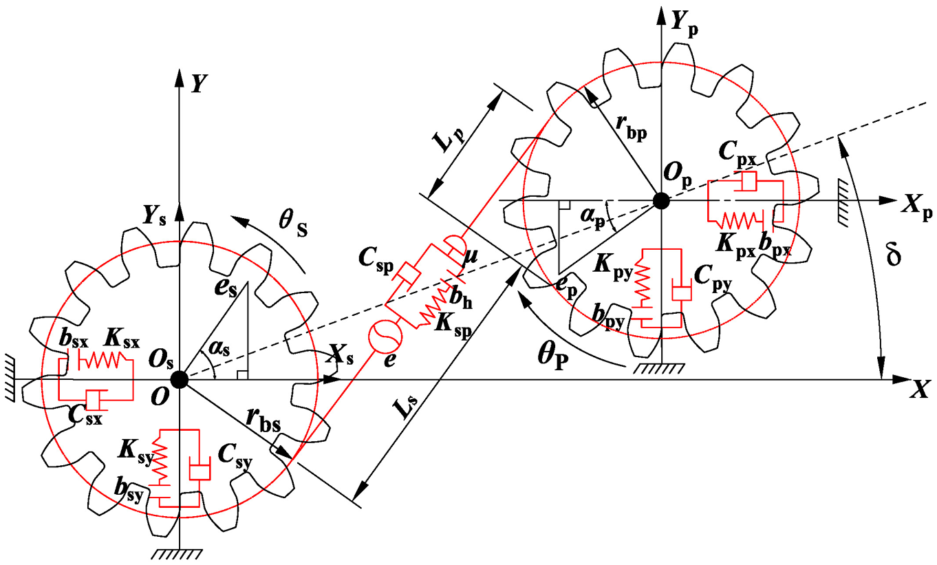
6-DOF bending–torsional coupling vibration model.

In Figure 1, the angular displacement of driving gear and driven gear is represented by θ_s and θ_p, respectively. The lateral displacement is represented by X_s and X_p, respectively. The longitudinal displacement is represented by Y_s and Y_p, respectively. The base circle radius is represented by r_bs and r_bp, respectively. The stiffness, half support clearance, and damping in the x and y directions of the driving gear are represented by K_sx, K_sy, b_sx, b_sy, C_sx, and C_sy, respectively. The stiffness, half support clearance, and damping in the x and y directions of the driven gear are represented by K_px, K_py, b_px, b_py, C_px, and C_py, respectively. Here, i is x and y. The comprehensive meshing error, time-varying mesh stiffness, half backlash, meshing damping, and friction coefficient of the gear pair are expressed by e(t), K_sp(t), b_h, C_sp, and μ, respectively. The friction arm of driving gear and driven gear is represented by L_s and L_p, respectively. The eccentricity errors of driving gear and driven gear are expressed by e_s and e_p, respectively. The initial phase angles of eccentricity errors are α_s and α_p, respectively. The phase angle between the driven gear and the driving gear is δ. The linear displacements x_s and x_p produced by the angular displacements of the driving gear and the driven gear on the meshing line can be shown in equation (1)

$$\{\begin{array}{c}{x}_{\mathrm{s}}={\theta }_{\mathrm{s}}{r}_{\mathrm{bs}}\hfill \\ \multicolumn{1}{c}{x_{\mathrm{p}}={\theta }_{\mathrm{p}}{r}_{\mathrm{bp}}}\end{array}$$

(1)

The comprehensive meshing error includes the static transmission error and eccentricity error of driving gear and driven gear. The harmonic period expansion of meshing transmission error by Fourier function can be expressed as follows

$$e\left(t\right)=E+\sum _{b=1}^l{e}_{\mathrm{s}}\sin (b{\omega }_{\mathrm{s}}t+{\alpha }_{\mathrm{s}})+\sum _{b=1}^l{e}_{\mathrm{p}}\sin (b{\omega }_{\mathrm{p}}t+{\alpha }_{\mathrm{p}})$$

(2)

In equation (2), E is the average value of static transmission error. α_s and α_p are the initial phase angles of the bth harmonic component, respectively. l is the number of harmonic terms expanded by Fourier. e_s and e_p are the eccentricity error. ω_s and ω_p are rotation frequency of driving gear and driven gear (rad/s).

The non-linear functions of backlash and support backlash can be expressed in equation (3)

$$\begin{array}{c}f(X,b_{\mathrm{h}})=\{\begin{array}{c}X-b_{\mathrm{h}}X>b_{\mathrm{h}}\hfill \\ \multicolumn{1}{c}{0\left|X\right|\le b_{\mathrm{h}}}\\ \multicolumn{1}{c}{X+b_{\mathrm{h}}X<-b_{\mathrm{h}},}\end{array}\hfill \\ f_{\mathrm{sx}}(X_{\mathrm{s}},b_{\mathrm{sx}})=\{\begin{array}{c}{X}_{\mathrm{s}}-b_{\mathrm{sx}}{X}_{\mathrm{s}}>b_{\mathrm{sx}}\hfill \\ \multicolumn{1}{c}{0\left|X_{\mathrm{s}}\right|\le b_{\mathrm{sx}}}\\ \multicolumn{1}{c}{X_{\mathrm{s}}+b_{\mathrm{sx}}{X}_{\mathrm{s}}<-b_{\mathrm{sx}},}\end{array}\hfill \\ f_{\mathrm{sy}}(Y_{\mathrm{s}},b_{\mathrm{sy}})=\{\begin{array}{c}{Y}_{\mathrm{s}}-b_{\mathrm{sy}}{Y}_{\mathrm{s}}>b_{\mathrm{sy}}\hfill \\ \multicolumn{1}{c}{0\left|Y_{\mathrm{s}}\right|\le b_{\mathrm{sy}}}\\ \multicolumn{1}{c}{Y_{\mathrm{s}}+b_{\mathrm{sy}}{Y}_{\mathrm{s}}<-b_{\mathrm{sy}}}\end{array}\hfill \\ f_{\mathrm{px}}(X_{\mathrm{p}},b_{\mathrm{px}})=\{\begin{array}{c}{X}_{\mathrm{p}}-b_{\mathrm{px}}{X}_{\mathrm{p}}>b_{\mathrm{px}}\hfill \\ \multicolumn{1}{c}{0\left|X_{\mathrm{p}}\right|\le b_{\mathrm{px}}}\\ \multicolumn{1}{c}{X_{\mathrm{p}}+b_{\mathrm{px}}{X}_{\mathrm{p}}<-b_{\mathrm{px}},}\end{array}\hfill \\ f_{\mathrm{py}}(Y_{\mathrm{p}},b_{\mathrm{py}})=\{\begin{array}{c}{Y}_{\mathrm{p}}-b_{\mathrm{py}}{Y}_{\mathrm{p}}>b_{\mathrm{py}}\hfill \\ \multicolumn{1}{c}{0\left|Y_{\mathrm{p}}\right|\le b_{\mathrm{py}}}\\ \multicolumn{1}{c}{Y_{\mathrm{p}}+b_{\mathrm{py}}{Y}_{\mathrm{p}}<-b_{\mathrm{py}}}\end{array}\hfill \end{array}$$

(3)

The dynamic meshing force of gear pair is defined as the sum of elastic restoring force and damping force, which can be expressed as follows

$$F_{\mathrm{N}}=K_{\mathrm{sp}}\left(t\right)f(X,b_{\mathrm{h}})+C_{\mathrm{sp}}\stackrel{·}{X}$$

(4)

In equation (4), X is the relative displacement of the gear pair’s meshing point.

The damping coefficient is expressed as follows

$$C_{\mathrm{sp}}=2\xi \sqrt{K_{\mathrm{m}}/(1/m_{\mathrm{s}}+1/m_{\mathrm{p}})}$$

(5)

In equation (5), ξ is the relative damping ratio of the meshing pair, m_s is the mass of the driving gear, m_p is the mass of the driven gear, and the relative damping ratio of the gear transmission system is generally 0.03 to 0.17.

Establishment of dynamic backlash b_h(t) based on fractal theory

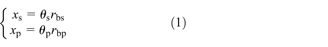
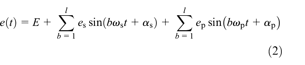
The W-M model of gear pair meshing based on the fractal theory is shown in Figure 2. A is the highest point of surface profile of gear 1. B is the highest point of surface profile of gear 2. The research in Yin et al. ²⁷ shows that the machined surface has fractal characteristics, and the tooth surface is also machined surface. The fractal formula of backlash can be defined by W-M function as follows

$$b_{\mathrm{h}}(t)=\sum _{k=0}^{+\infty }{{\lambda }_{\mathrm{b}}}^{(D-2)k}\sin ({{\lambda }_{\mathrm{b}}}^{k}t);{\lambda }_{\mathrm{b}}>1,1<D<2$$

(6)

In equation (6), b_h(t) is the backlash varying with the time. λ_b is the characteristic scale coefficient. D is the fractal dimension, and only two-dimensional fractal is considered. k is the contact coefficient. t is time.

Figure 2.

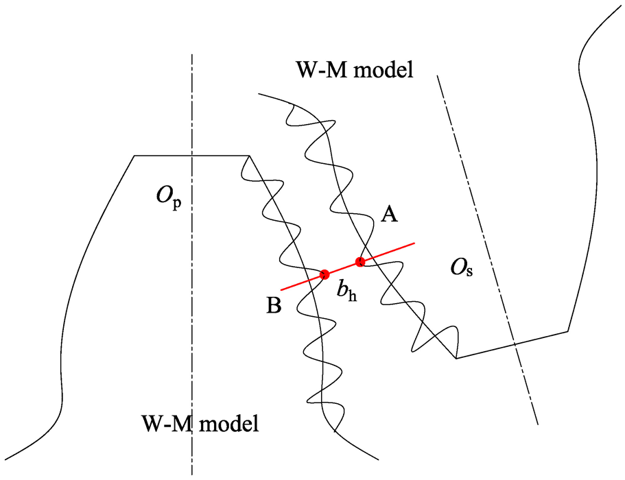
W-M model of gear pair meshing.

Using equation (6), the simulation of backlash under different fractal dimensions is shown in Figure 3. Here, λ is 1.5 and D is 1.1–1.9, respectively. The larger the fractal dimension D, the more complex the micro morphology of W-M simulation. The curve changes more dramatically with the increase in fractal dimension D. The larger the fractal dimension D, the smoother the tooth surface and the smaller the backlash. The average backlash b_hm with different fractal dimension D is shown in Table 1.

Figure 3.

The simulation of backlash (b_h) with different fractal dimensions (D): (a) D = 1.1, (b) D = 1.2, (c) D = 1.3, (d) D = 1.4, (e) D = 1.5, (f) D = 1.6, (g) D = 1.7, (h) D = 1.8, and (i) D = 1.9.

Table 1.

The average backlash b_hm in different fractal dimension D.

D	1.1	1.2	1.3	1.4	1.5	1.6	1.7	1.8	1.9
b hm	1.5472	0.9744	0.6140	0.3872	0.2444	0.1544	0.0978	0.0620	0.0394

Calculation of time-varying tooth surface friction based on EHL

The schematic diagram of gear force analysis is shown in Figure 4.

Figure 4.

Friction analysis of gear pair.

In the process of gear transmission, the tooth surface will be affected by the dynamic meshing force F_N along the direction of the meshing line and the friction force F_f perpendicular to the meshing line. XY is the theoretical meshing line length. AD is the actual meshing line length. r_as and r_ap are the top circle radius of driving gear and driven gear. r_s and r_p are the pitch circle radius of driving gear and driven gear. ω_s and ω_p are the rotation frequency of driving gear and driven gear, rad/s. α_n is the meshing angle.

From the geometric relationship of gear transmission, we can get the length XY of theoretical meshing line, the length AD of actual meshing line, the distance XA between the start end of actual and theoretical meshing line, and the distance YD between the end of actual and theoretical meshing line. The calculation expression is as follows

$$\{\begin{array}{c}\mathrm{XY}=(r_{\mathrm{s}}+r_{\mathrm{p}})\sin {\alpha }_{\mathrm{n}}\hfill \\ \multicolumn{1}{c}{\mathrm{AD}=\sqrt{r_{\mathrm{as}}^2-r_{\mathrm{bs}}^2}+\sqrt{r_{\mathrm{ap}}^2-r_{\mathrm{bp}}^2}-(r_{\mathrm{s}}+r_{\mathrm{p}})\sin {\alpha }_{\mathrm{n}}}\\ \multicolumn{1}{c}{\mathrm{XA}=(r_{\mathrm{s}}+r_{\mathrm{p}})\sin {\alpha }_{\mathrm{n}}-\sqrt{r_{\mathrm{ap}}^2-r_{\mathrm{bp}}^2}}\\ \multicolumn{1}{c}{\mathrm{YD}=(r_{\mathrm{s}}+r_{\mathrm{p}})\sin {\alpha }_{\mathrm{n}}-\sqrt{r_{\mathrm{as}}^2-r_{\mathrm{bs}}^2}}\\ \multicolumn{1}{c}{P_{\mathrm{b}}=\frac{2\mathrm{\pi }{r}_{\mathrm{bs}}}{Z_{\mathrm{s}}}=\frac{2\mathrm{\pi }{r}_{\mathrm{bp}}}{Z_{\mathrm{p}}}}\end{array}$$

(7)

In equation (7), P_b is the pitch of gear. Z_s and Z_p are the number of teeth of driving gear and driven gear, respectively.

Therefore, the expression of the friction arm can be derived as follows

$$\{\begin{array}{c}{L}_{\mathrm{s}}(t)=\mathrm{XA}+P_{\mathrm{b}}+mod({\omega }_{\mathrm{s}}{r}_{\mathrm{bs}}t,P_{\mathrm{b}})\hfill \\ \multicolumn{1}{c}{L_{\mathrm{p}}(t)=\mathrm{YD}+mod({\omega }_{\mathrm{p}}{r}_{\mathrm{bp}}t,P_{\mathrm{b}})}\end{array}$$

(8)

In equation (8), L_s and L_p are the time-varying friction arms of the driving gear and driven gear, respectively, mod (·) is the complementary function.

The relative velocity u_e of two meshing contact tooth surfaces at any position is shown in equation (9)

$$u_{\mathrm{e}}\left(t\right)=L_{\mathrm{s}}\left(t\right){\omega }_{\mathrm{s}}-L_{\mathrm{p}}\left(t\right){\omega }_{\mathrm{p}}$$

(9)

Since the direction of friction force will change at the node, the direction coefficient λ can be used to represent the direction change. The direction coefficient is defined as

$$\lambda (t)=\mathrm{sgn}\left(u_{\mathrm{e}}\left(t\right)\right)=\{\begin{array}{c}\begin{array}{cc}1\hfill & u_{\mathrm{e}}\left(t\right)<0\hfill \end{array}\hfill \\ \multicolumn{1}{c}{\begin{array}{cc}0\hfill & u_{\mathrm{e}}\left(t\right)=0\hfill \end{array}}\\ \multicolumn{1}{c}{\begin{array}{cc}-1\hfill & u_{\mathrm{e}}\left(t\right)>0\hfill \end{array}}\end{array}$$

(10)

In equation (10), sgn(·) is a symbolic function.

The calculation formula of Coulomb’s law friction model is as follows

$$\begin{array}{c}\multicolumn{1}{c}{\mu (t)={\mu }_0\mathrm{sign}(\mathrm{AP}-mod(r_{\mathrm{bs}}{\omega }_{\mathrm{s}}t,P_{\mathrm{b}}))}\\ =\{\begin{array}{c}\begin{array}{cc}{\mu }_0\hfill & \mathrm{AP}<mod(r_{\mathrm{bs}}{\omega }_{\mathrm{s}}t,P_{\mathrm{b}})\hfill \end{array}\hfill \\ \multicolumn{1}{c}{\begin{array}{cc}0\hfill & \mathrm{AP}=mod(r_{\mathrm{bs}}{\omega }_{\mathrm{s}}t,P_{\mathrm{b}})\hfill \end{array}}\\ \multicolumn{1}{c}{\begin{array}{cc}-{\mu }_0\hfill & \mathrm{AP}>mod(r_{\mathrm{bs}}{\omega }_{\mathrm{s}}t,P_{\mathrm{b}})\hfill \end{array}}\end{array}\hfill \end{array}$$

(11)

In equation (11), μ₀ is the amplitude of friction coefficient.

The time-varying sliding friction force of tooth surface according to Coulomb’s law can be expressed as follows

$$F_f\left(t\right)=\lambda \left(t\right)\mu \left(t\right)F_{\mathrm{N}}$$

(12)

In equation (12), μ is the friction coefficient.

In aviation standard, the empirical formula of friction coefficient at any meshing point K synthesized according to the actual test results is as follows

$$\mu =0.12{\left(\frac{W_{\mathrm{t}}{R}_{\mathrm{a}}}{2{\nu }_0{u}_{\mathrm{sp}}R}\right)}^{0.25}$$

(13)

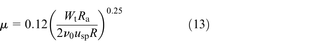
In equation (13), ν₀ is the initial viscosity of the lubricating oil (Pa/s). W_t is the tangential load per unit tooth width (N/mm). u_sp is the entrainment velocity (m/s). R is the comprehensive curvature radius of the gear pair (mm). R_a is the mean value of tooth surface roughness (μm). Ignoring the effect of roughness, R_a is equal to zero.

The friction coefficient is related to the geometric shape of the teeth, the surface roughness of the teeth, the relative sliding velocity of the teeth, the contact stress between the teeth, and the lubrication of the system, so it is difficult to accurately predict the friction coefficient. When the lubrication effect of tooth surface is considered, the gear contact problem becomes the linear contact EHL problem. Therefore, the friction coefficient is calculated by EHL theory.

By solving Reynolds equation, viscous pressure equation, dense pressure equation, energy balance equation, and load equation, the oil film pressure distribution and film thickness distribution are obtained. Combined with Ree–Eyring fluid equation, the oil film shear stress distribution is calculated, and then, the friction force and friction coefficient between two contact surfaces are obtained. It is assumed that the tooth surface is completely smooth, that is, the gear is in the state of complete EHL. In the lubrication analysis, the influence of temperature effect is ignored, and it is considered that the oil film thickness has not changed.

The Reynolds equation is

$$\{\begin{array}{c}\frac{\partial }{\partial x}\left[{\left(\frac{\rho }{\nu }\right)}_e{h}^3\frac{\partial p}{\partial x}\right]=12u_{\mathrm{sp}}\frac{\partial ({\rho }^{*}h)}{\mathrm{dx}}\hfill \\ u_{\mathrm{sp}}=(u_{\mathrm{s}}+u_{\mathrm{p}})/2\hfill \\ p_{x_{\mathrm{in}}}=p_{x_{\mathrm{out}}}=p_x=0\hfill \\ \frac{\partial p}{\partial x}|x_{\mathrm{out}}=0\hfill \end{array}$$

(14)

In equation (14), x is the tangent direction of tooth surface. ρ is the density of lubricating oil (kg/m³). h is the oil film thickness (m). p is oil film pressure (Pa). ν is the viscosity of Ree-Eyring fluid (Pa·s). u_sp is the entrainment velocity (m/s), u_s, u_p are the tangential velocity of lubricating oil along gear axis (m/s). x_in and x_out are the entrance and exit positions of the calculation area in the x-direction. ρ* and (ρ/ν) _e are the equivalent parameters. The equivalent parameters are defined in equation (15)

$$\{\begin{array}{c}{\left(\frac{\rho }{\nu }\right)}_e=12({\nu }_e\frac{\rho {\prime }_e}{{\nu \prime }_e}-{\rho ″}_e)\hfill \\ {\rho }^{*}=[{\rho \prime }_e{\nu }_e(u_{\mathrm{s}}-u_{\mathrm{p}})+{\rho }_e{u}_{\mathrm{s}}]/u_{\mathrm{sp}}\hfill \\ {\rho }_e=\frac{1}{h}\underset{0}{\overset{h}{\int }}\rho \mathrm{d}z\hfill \\ {\rho \prime }_e=\frac{1}{h^2}\underset{0}{\overset{h}{\int }}\rho \underset{0}{\overset{z}{\int }}\frac{\mathrm{dz}\prime }{{\nu }^{*}}\mathrm{d}z\hfill \\ {\rho ″}_e=\frac{1}{h^3}\underset{0}{\overset{h}{\int }}\rho \underset{0}{\overset{z}{\int }}\frac{z\prime \mathrm{d}z\prime }{{\nu }^{*}}\mathrm{d}z\hfill \\ \frac{1}{{\nu }_e}=\frac{1}{h}\underset{0}{\overset{h}{\int }}\frac{\mathrm{d}z}{{\nu }^{*}}\hfill \\ \frac{1}{{\nu \prime }_e}=\frac{1}{h^2}\underset{0}{\overset{h}{\int }}\frac{z\mathrm{d}z}{{\nu }^{*}}\hfill \end{array}$$

(15)

The boundary conditions for the differential equations are p(x_in) = 0, p(x_out) = 0, p(x_in) > 0, and (x_in < x < x_out). ν* is the equivalent viscosity of lubricating oil (Pa·s).

The film thickness equation is as follows

$$\{\begin{array}{c}h(x)=h_0+\frac{x^2}{2R}+\delta (x)\hfill \\ \delta (x)=-\frac{2}{\pi E\prime }\underset{x_{\mathrm{in}}}{\overset{x_{\mathrm{out}}}{\int }}p(\mathrm{Sr})\ln (x-\mathrm{Sr}{)}^2\mathrm{d}\mathrm{Sr}+C_d\hfill \end{array}$$

(16)

In equation (16), h₀ is the central film thickness (m) of the two gears without meshing deformation, which can be determined by the load balance condition. R is the comprehensive curvature radius (m). δ(x) is the elastic deformation displacement (m) due to the contact pressure of the tooth surface. E′ is the comprehensive elastic modulus (Pa) of the two gears. Sr is the sliding roll ratio when the gear is engaged. C_d is the viscosity pressure coefficient of Cameron’s viscosity pressure formula (m²/N), C_d = χ/15, and χ is the viscosity pressure coefficient of Barus’ viscosity pressure formula (m²/N).

The viscous pressure equation and the dense pressure equation can be expressed as follows

$$\{\begin{array}{c}\nu ={\nu }_0\exp \{(\ln {\nu }_0+9.67)[-1+(1+5.1\times {10}^{-9}p{)}^{z_0}]\}\hfill \\ \rho ={\rho }_0[1+\frac{0.6\times {10}^{-9}p}{1+1.7\times {10}^{-9}p}]\hfill \\ z_0=\chi /[5.1\times {10}^{-9}\times (\ln {\nu }_0+9.67)]\hfill \end{array}$$

(17)

In equation (17), ν₀ is the initial viscosity of the lubricating oil (Pa·s). ρ₀ is the initial density of the lubricant (kg/m³).

The load balance equation can be expressed as follows

$$\{\begin{array}{c}{c}_w(t)W=\underset{x_{\mathrm{in}}}{\overset{x_{\mathrm{out}}}{\int }}p(x)\mathrm{dx}\hfill \\ \multicolumn{1}{c}{c_w(t)=\{\begin{array}{c}\frac{1}{3}(1+\frac{\mathrm{Sr}-x_{\mathrm{in}}}{x_0})\begin{array}{c}{x}_{\mathrm{in}}\le \mathrm{Sr}\le x_{\mathrm{in}}+x_0\hfill \end{array}\hfill \\ \multicolumn{1}{c}{1\begin{array}{c}\begin{array}{c}{x}_{\mathrm{in}}+{\mathrm{x}}_0\le \mathrm{Sr}\le x_{\mathrm{out}}-x_0\hfill \end{array}\hfill \end{array}}\\ \multicolumn{1}{c}{\frac{1}{3}(1+\frac{\mathrm{Sr}-x_{\mathrm{out}}}{x_0})\begin{array}{c}{x}_{\mathrm{out}}-x_0\le \mathrm{Sr}\le x_{\mathrm{out}}\hfill \end{array}}\end{array}}\\ \multicolumn{1}{c}{x_0=\mathrm{\pi }{m}_{\mathrm{n}}\cos {\alpha }_{\mathrm{n}}(\epsilon -1)}\end{array}$$

(18)

In equation (18), W is the equivalent cylinder external load (N). c_w(t) is the load factor of gear. Taking the meshing line of gear transmission as the coordinate axis and the node as the origin, x_in and x_out are the coordinates of entering and leaving the meshing point, respectively, m_n is the modulus and ε is the gear coincidence degree.

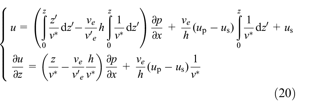
The constitutive equation of Ree-Eyring fluid can be expressed as follows

$$\{\begin{array}{c}\tau ={\nu }^{*}\frac{\partial u}{\partial z}\hfill \\ \multicolumn{1}{c}{{\nu }^{*}=\nu (\tau /{\tau }_0)/\sin \mathrm{h}(\tau /{\tau }_0)}\end{array}$$

(19)

In equation (19), τ is the shear stress of oil film in x-direction (Pa). u is the velocity of lubricating oil in x-direction (m/s). τ₀ is the shear stress of Ree–Eyring fluid (Pa).

The formula of velocity and velocity gradient derived from the motion equation of fluid particle can be expressed in equation (20)

$$\{\begin{array}{c}u=(\underset{0}{\overset{z}{\int }}\frac{z\prime }{v^{*}}\mathrm{d}z\prime -\frac{v_e}{{v\prime }_e}h\underset{0}{\overset{z}{\int }}\frac{1}{v^{*}}\mathrm{d}z\prime )\frac{\partial p}{\partial x}+\frac{v_e}{h}(u_{\mathrm{p}}-u_{\mathrm{s}})\underset{0}{\overset{z}{\int }}\frac{1}{v^{*}}\mathrm{d}z\prime +u_{\mathrm{s}}\hfill \\ \frac{\partial u}{\partial z}=(\frac{z}{v^{*}}-\frac{v_e}{{v\prime }_e}\frac{h}{v^{*}})\frac{\partial p}{\partial x}+\frac{v_e}{h}(u_{\mathrm{p}}-u_{\mathrm{s}})\frac{1}{v^{*}}\hfill \end{array}$$

(20)

The friction force on the contact tooth surface of the gear and the velocity distribution of the lubricant are shown in Figure 5.

Figure 5.

Schematic diagram of velocity distribution and friction force.

Here, the sliding friction is mainly generated in the contact area (−b, b). F₁ and F₂ are the friction force on the surface of the two tooth surfaces, respectively. The sliding friction coefficient of the gear based on the EHL model can be expressed as follows

$$\mu =\frac{F_1+F_2}{2W}=\frac{\underset{-b}{\overset{b}{\int }}\tau {|}_{z=0}\mathrm{d}x+\underset{-b}{\overset{b}{\int }}\tau {|}_{z=h}\mathrm{d}x}{2W}$$

(21)

In equation (21), $F_1={\int }_{-b}^b\tau {|}_{z=0}\mathrm{d}x$ and $F_2={\int }_{-b}^b\tau {|}_{z=h}\mathrm{d}x$ .

The above mathematical model is dimensionless. Then, the multi-grid method is used to solve the pressure, and the numerical method is used to solve the friction coefficient and friction.

In order to verify the correctness of the proposed sliding friction coefficient, this article gives the friction coefficient calculated by EHL empirical formula in Xu et al. ³⁴ and makes a comparison. Calculation model expression of friction coefficient based on EHL empirical formula proposed by Xu et al. ³⁴ is as follows

$$\mu =e^{f(\mathrm{sr},P_{\mathrm{h}},{\nu }_{\mathrm{m}},R_{\mathrm{rms}})}{P}_{\mathrm{h}}^{b2}{\left|\mathrm{Sr}\right|}^{b3}{u}_{\mathrm{sp}}^{b6}{\nu }_{\mathrm{m}}^{b7}{R}^{b8}$$

(22)

In equation (22), P_h is the maximum contact Hertz stress (GPa). R_rms is the root mean square (RMS) value of roughness.

f (Sr, P_h, ν_m, R_rms) is calculated in equation (23) as follows

$$\begin{array}{c}\multicolumn{1}{c}{f(\mathrm{Sr},P_{\mathrm{h}},{\nu }_{\mathrm{m}},R_{\mathrm{rms}})=b_1+b_4\left|\mathrm{Sr}\right|P_{\mathrm{h}}{\log }_{10}({\nu }_{\mathrm{m}})}\\ +b_5{e}^{-\left|\mathrm{sr}\right|P_{\mathrm{h}}{\log }_{10}({\nu }_{\mathrm{m}})}+b_9{e}^{R_{\mathrm{rms}}}\hfill \end{array}$$

(23)

The values of b₁, b₂, …, b₉ are shown in Table 2.

Table 2.

Parameters of EHL friction coefficient calculation model.

Parameters	b 1	b 2	b 3	b 4	b 5	b 6	b 7	b 8	b 9
Value	−8.9165	1.03303	1.03608	−0.3541	2.81208	−0.1006	0.75276	−0.3910	0.62031

EHL: elasto-hydrodynamic lubrication.

Maximum Hertz contact stress can be expressed as

$$P_{\mathrm{h}}=\sqrt{\frac{W\prime E\prime }{2\mathrm{\pi }R}}$$

(24)

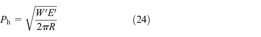
In equation (24), E′ is the comprehensive elasticity modulus, GPa, and calculated as follows

$$E\prime =\frac{2}{\frac{(1-{\mu }_{\mathrm{s}}^2)}{E_{\mathrm{s}}}+\frac{(1-{\mu }_{\mathrm{p}}^2)}{E_{\mathrm{p}}}}$$

(25)

In equation (25), μ_s and μ_p are Poisson’s ratio of driving gear and driven gear, respectively. E_s and E_p are the elastic modulus of driving gear and driven gear, respectively.

The instantaneous velocity u_s and u_p at any meshing point is calculated as follows

$$\{\begin{array}{c}{u}_{\mathrm{s}}={\omega }_{\mathrm{s}}{\rho }_{\mathrm{s}}={\omega }_{\mathrm{s}}(s+\mathrm{XA})\hfill \\ \multicolumn{1}{c}{u_{\mathrm{p}}={\omega }_{\mathrm{p}}{\rho }_{\mathrm{p}}={\omega }_{\mathrm{p}}(\mathrm{XY}-s-\mathrm{XA})}\end{array}$$

(26)

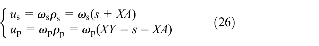
In equation (26), ρ_s and ρ_p are the curvature radius. s is the distance between the instantaneous meshing point and the actual meshing starting point, m.

The sliding roll ratio Sr, the tooth surface relative sliding velocity u_e, the entrainment velocity u_sp, and the rolling velocity u_r are calculated in equation (27)

$$\{\begin{array}{c}\mathrm{Sr}=\frac{u_{\mathrm{e}}}{u_{\mathrm{sp}}}=\frac{2u_{\mathrm{e}}}{u_{\mathrm{r}}}=\frac{2|u_{\mathrm{s}}-u_{\mathrm{p}}|}{u_{\mathrm{s}}+u_{\mathrm{p}}}\hfill \\ u_{\mathrm{e}}=|u_{\mathrm{s}}-u_{\mathrm{p}}|\hfill \\ u_{\mathrm{r}}=u_{\mathrm{s}}+u_{\mathrm{p}}\hfill \end{array}$$

(27)

Here, regardless of the influence of roughness, RMS value of roughness R_rms = 0.0 μm. Mobil dte24 anti-wear lubricating oil is selected, and its relevant parameters are shown in Table 3.

Table 3.

Lubricating oil parameters.

Parameters	Values	Unit
Lubricating oil initial density ρ0	871	kg/m3
Lubricating oil initial viscosity v0	0.0527	Pa/s
Lubricating oil kinematic viscosity v	31.5	cSt
Ree–Eyring fluid viscosity v*	0.824	Pa/s
Lubricating oil viscosity pressure coefficient χ	2.389 × 108	m2/N
Ree–Eyring fluid shear stress τ0	1.0 × 106	Pa
Elastic modulus Es, Ep	227 × 109	Pa
Poisson ratio μs, μp	0.3

In order to compare the calculation results of different friction coefficient models, the power is 100 kW and the input speed n_p is 5000 r/min. The change curve of tooth surface friction coefficient with slip roll ratio sr is shown in Figure 6. Figure 6(a) and (b) shows the curve of sliding friction coefficient with the entrainment velocity at 1.0, 2.0, and 3.0 m/s. EHL model comprehensively considers the load distribution, relative sliding velocity of tooth surface, gear surface morphology, and lubrication conditions. In this article, the friction coefficient calculation model based on EHL is used. From Figure 6, due to the calculation of EHL model without considering surface roughness, and assuming that the lubrication state is complete EHL, the value of sliding friction coefficient obtained by EHL model is smaller than that of Coulomb model. The coefficient of sliding friction calculated by EHL model increases first and then decreases with the decrease in sliding roll ratio Sr. The coefficient of sliding friction decreases with the increase in entrainment velocity u_sp.

Figure 6.

Change curve of friction coefficient with slip roll ratio Sr: (a) u_sp = 1.0 m/s, (b) u_sp = 2.0 m/s, and (c) u_sp = 3.0 m/s.

Calculation of time-varying mesh stiffness based on LTCA

LTCA method is used to calculate the time-varying mesh stiffness, and the results are compared with those of Ishikawa method. LTCA model of driving gear and driven gear is shown in Figure 7.

Figure 7.

LTCA model.

Under the load P, the driving gear goes through an approach Z. Due to the tooth deformation, contact load will become distributed. After contact deformation, the state can be described by the following equation for the tooth pair k

$$\{\begin{array}{c}\sum _{j=1}^n{P}_{j\mathrm{I}}+\sum _{j=1}^n{P}_{j\Pi }=P\left(P_j(j=1,2,\dots ,n)\right)\hfill \\ \multicolumn{1}{c}{[F{]}_k[P_j{]}_k+[w{]}_k=[Z]+[d_j{]}_k}\end{array}$$

(28)

In equation (28), j_k is a point along the relative principal direction, k = I, II, [F] _k is the normal flexibility coefficient matrix of the tooth pair k, [d_j] _k = [d_1k, d_2k, …, d_ik, …, djk_jk, d_nk]^T is the tooth surface clearance to contact the discrete point j of the ellipse long axis of the tooth pair k. [Z] = [1, 1, …, 1, …, 1]^T is the Normal displacement of gear teeth under load. [P_j] _k = [P_1k, P_2k, …, P_ik, …, Pjk_jk, P_nk]^T is the normal load to contact the discrete point j of the ellipse long axis of the tooth pair k. If p_jk > 0, then d_jk = 0. if p_jk = 0, then d_jk > 0. The tooth surface initial clearance w of gears I and II is [w] _k = [δ_T] _k +[b] _k (k = I, II). [w] _k = [w_1k, w_2k, …, w_ik, …, wjk_jk, w_nk]^T, [b] _k =[b₁, b₂, …, b_i, …, bn_n]^T, [δ_T] _k =[1, 1, …, 1, …, 1]^T. n is the number of discrete points. b_j is the tooth surface normal clearance (j = 1, …, n). δ_T is the geometric transmission error.

LTCA calculation is carried out for all the meshing positions in a meshing cycle, and Z, [P], and [d] are obtained. Z is the normal linear displacement transmission error of the gear after deformation under the normal load P of the current contact position, which is transformed into the angular displacement error Δφ_sp.

The elastic deformation of the gear teeth under normal load, including the geometric bending deformation δ_B of the gear teeth, the elastic deformation δ_M at the root of the gear teeth, and the contact deformation δ_C at the meshing point, is obtained. The relationship between the comprehensive elastic deformation Δφ_sp[T_sp(k)] and the transmission torque T_sp(k) of the gear pair is as follows

$$\mathrm{\Delta }{\phi }_{\mathrm{sp}}\left[T_{\mathrm{sp}}\left(k\right)\right]=\frac{T_{\mathrm{sp}}\left(k\right)}{\left|T_{\mathrm{sp}}\left(k\right)\right|}(a+b{T}_{\mathrm{sp}}\left(k\right)+c{T}_{\mathrm{sp}}{\left(k\right)}^{\frac{2}{3}})$$

(29)

In equation (29), a, b, and c are the constant terms in the formula, which are determined by the geometric parameters of the gear and the coordinates of the meshing position, T_sp(k) (k = 1,2, …,5) is the torque of the kth meshing position in a meshing cycle. δ_B = a, δ_M = bT_sp(k), and δ_C = cT_sp(k)^2/3.

Through the finite element calculation and the gear geometric contact simulation analysis program, when the gear pair is in the meshing position k, solving equation (27), the load transmission error Δδ_T (0.1T_sp(k)), Δδ_T (0.5T_sp(k)), and Δδ_T (0.9T_sp(k)) are obtained. The results are brought into equation (28), and the coefficients a, b, and c are obtained, and the function relation between the loaded deformation of the driving gear and driven gear and the nominal load is obtained. The time-varying mesh stiffness of driving gear and driven gear is obtained. The following equation (30) is satisfied with the integrated time-varying mesh stiffness K_sp of driving gear and driven gear with the corresponding angular error Δφ_sp(T_sp(k))

$$K_{\mathrm{sp}}=\frac{T_{\mathrm{sp}}\left(k\right)}{r_{\mathrm{bs}}^2\mathrm{\Delta }{\phi }_{\mathrm{sp}}\left[T_{\mathrm{sp}}\left(k\right)\right]}$$

(30)

The discrete value of the time-varying mesh stiffness calculated by LTCA is expanded into a harmonic periodic function with ω as the fundamental frequency by Fourier series. Its mathematical form can be described as follows

$$K_{\mathrm{sp}}\left(t\right)=K_{\mathrm{m}}+\sum _{a=1}^l{K}_{\mathrm{a}}\sin (a\omega t+{\psi }_{\alpha })$$

(31)

In equation (31), K_m is the average value of the fluctuation of the meshing stiffness. ω is the meshing frequency of the gear pair, and the meshing period is T=2π/ω. l is the order of the harmonic term expanded by the Fourier series. K_a is the stiffness amplitude of the ath (a = 1, 2, 3, …, l) harmonic component. ψ_α is the initial phase angle of meshing of the ath (a = 1, 2, 3, …, l) harmonic component.

The calculation formula of Ishikawa method is that the contact gear is equivalent to the cantilever beam composed of rectangle and trapezoid to calculate the deformation, and the dangerous section of the gear is defined as the length of rectangle, the specific calculation will not be described here. Figure 8(a) shows the comparison curve between LTCA calculation results and Ishikawa calculation results. The time-varying mesh stiffness including the friction factor of tooth surface is calculated, as shown in Figure 8(b). The time-varying mesh stiffness of the gear considering the friction of the tooth surface is larger than that without considering the friction, and the variation range is about 8%. This is because when the friction factor of tooth surface is considered, the friction makes the meshing stiffness of tooth pair increase in the meshing stage and decrease in the meshing out stage. The larger the friction coefficient is, the greater the variation of stiffness will be.

Figure 8.

Time-varying meshing stiffness curve: (a) without tooth surface friction and (b) with tooth surface friction.

Establishment of differential equation of bending torsional coupling vibration based on LPM

Based on the Lumped Parameter Theory (LPM), a multi-clearance coupled bending torsional vibration model is established, and the differential equations of the system are obtained as follows (equation (32)). Here, it is assumed that the transmission shaft has enough stiffness, ignoring the torsional stiffness and torsional damping of the shaft, and ignoring the elastic deformation of the shaft

$$\{\begin{array}{c}{m}_{\mathrm{s}}{\stackrel{··}{X}}_{\mathrm{s}}+K_{\mathrm{sx}}{f}_{\mathrm{sx}}(X_{\mathrm{s}},b_{\mathrm{sx}})+C_{\mathrm{sx}}{\stackrel{·}{X}}_{\mathrm{s}}=-(\sin \phi +\lambda u\cos \phi )F_{\mathrm{N}}\hfill \\ \multicolumn{1}{c}{m_{\mathrm{s}}{\stackrel{··}{Y}}_{\mathrm{s}}+K_{\mathrm{sy}}{f}_{\mathrm{sy}}(Y_{\mathrm{s}},b_{\mathrm{sy}})+C_{\mathrm{sy}}{\stackrel{·}{Y}}_{\mathrm{s}}=-(\cos \phi +\lambda u\sin \phi )F_{\mathrm{N}}}\\ \multicolumn{1}{c}{I_{\mathrm{s}}{\stackrel{··}{\theta }}_{\mathrm{s}}+(1+u\lambda L_{\mathrm{s}j}/r_{\mathrm{bs}})r_{\mathrm{bs}}{F}_{\mathrm{N}}=T_{\mathrm{in}}}\\ \multicolumn{1}{c}{m_{\mathrm{p}}{\stackrel{··}{X}}_{\mathrm{p}}+K_{\mathrm{px}}{f}_{\mathrm{px}}(X_{\mathrm{p}},b_{\mathrm{px}})+C_{\mathrm{px}}{\stackrel{·}{X}}_{\mathrm{p}}=(\sin \phi +\lambda u\cos \phi )F_{\mathrm{N}}}\\ \multicolumn{1}{c}{m_{\mathrm{p}}{\stackrel{··}{Y}}_{\mathrm{p}}+K_{\mathrm{py}}{f}_{\mathrm{py}}(Y_{\mathrm{p}},b_{\mathrm{py}})+C_{\mathrm{py}}{\stackrel{·}{X}}_{\mathrm{p}}=(\cos \phi +\lambda u\sin \phi )F_{\mathrm{N}}}\\ \multicolumn{1}{c}{I_{\mathrm{p}}{\stackrel{··}{\theta }}_{\mathrm{p}}-(1-u\lambda L_{\mathrm{p}j}/r_{\mathrm{bp}})r_{\mathrm{bp}}{F}_{\mathrm{N}}=T_{\mathrm{out}}}\end{array}$$

(32)

In equation (32), $\phi =\delta -{\alpha }_{\mathrm{n}}$ , φ is the projection angle. I_s is the moment inertia of driving gear. I_p is the moment inertia of driven gear. T_in is the input torque. T_out is the output torque.

In order to facilitate comparison and analysis, making the solution of the system in the same order of magnitude, dimension time τ = ω_nt and displacement nominal scale b_c are introduced. Here, ${\omega }_{\mathrm{n}}=\sqrt{K_{\mathrm{m}}(I_{\mathrm{s}}{r}_{\mathrm{p}}^2+I_{\mathrm{p}}{r}_{\mathrm{s}}^2)/(I_{\mathrm{s}}{I}_{\mathrm{p}})}$ . The dimensional displacement, velocity, and acceleration are $X=\overline{X}{b}_c$ , $\stackrel{·}{X}=\stackrel{·}{\overline{X}}{\omega }_{\mathrm{n}}{b}_{\mathrm{c}}$ , and $\stackrel{··}{X}=\stackrel{··}{\overline{X}}{\omega }_{\mathrm{n}}^2{b}_{\mathrm{c}}$ , respectively. The dimensional backlash, dimensional rotational speed, dimensionless angular velocity can be expressed as $b_{\mathrm{h}}={\overline{b}}_{\mathrm{h}}{b}_{\mathrm{c}}$ , $\mathrm{\Omega }=\omega /{\omega }_{\mathrm{n}}$ , ${\mathrm{\Omega }}_{\mathrm{s}}={\omega }_{\mathrm{s}}/{\omega }_{\mathrm{n}}$ , and ${\mathrm{\Omega }}_{\mathrm{p}}={\omega }_{\mathrm{p}}/{\omega }_{\mathrm{n}}$ , respectively.

The dimensional comprehensive meshing error of gear pair can be expressed as follows (equation (33))

$$\begin{array}{c}\multicolumn{1}{c}{\overline{e}\left(t\right)=\frac{\overline{E}}{b_c}+\frac{e_{\mathrm{s}}}{b_c}\sum _{b=1}^l\sin (b{\mathrm{\Omega }}_{\mathrm{s}}\tau +{\alpha }_{\mathrm{s}})}\\ +\frac{e_{\mathrm{p}}}{b_c}\sum _{b=1}^l\sin (b{\mathrm{\Omega }}_{\mathrm{p}}\tau +{\alpha }_{\mathrm{p}})\hfill \end{array}$$

(33)

The non-linear function of dimension clearance of gear pair can be expressed as follows (equation (34))

$$\{\begin{array}{c}f(\overline{X},{\overline{b}}_{\mathrm{h}})=\{\begin{array}{c}\overline{X}-{\overline{b}}_{\mathrm{h}}\overline{X}>{\overline{b}}_{\mathrm{h}}\hfill \\ \multicolumn{1}{c}{0\left|\overline{X}\right|\le {\overline{b}}_{\mathrm{h}}}\\ \multicolumn{1}{c}{\overline{X}+{\overline{b}}_{\mathrm{h}}\overline{X}<-{\overline{b}}_{\mathrm{h}}}\end{array};\hfill \\ \multicolumn{1}{c}{f_{\mathrm{sx}}({\overline{X}}_{\mathrm{s}},{\overline{b}}_{\mathrm{sx}})=\{\begin{array}{c}{\overline{X}}_{\mathrm{s}}-{\overline{b}}_{\mathrm{sx}}{\overline{X}}_{\mathrm{s}}>{\overline{b}}_{\mathrm{sx}}\hfill \\ \multicolumn{1}{c}{0\left|{\overline{X}}_{\mathrm{s}}\right|\le {\overline{b}}_{\mathrm{sx}}}\\ \multicolumn{1}{c}{{\overline{X}}_{\mathrm{s}}+{\overline{b}}_{\mathrm{sx}}{\overline{X}}_{\mathrm{s}}<-{\overline{b}}_{\mathrm{sx}}}\end{array};f_{\mathrm{sy}}({\overline{Y}}_{\mathrm{s}},{\overline{b}}_{\mathrm{sy}})=\{\begin{array}{c}{\overline{Y}}_{\mathrm{s}}-{\overline{b}}_{\mathrm{sy}}{\overline{Y}}_{\mathrm{s}}>{\overline{b}}_{\mathrm{sy}}\hfill \\ \multicolumn{1}{c}{0\left|{\overline{Y}}_{\mathrm{s}}\right|\le {\overline{b}}_{\mathrm{sy}}}\\ \multicolumn{1}{c}{{\overline{Y}}_{\mathrm{s}}+{\overline{b}}_{\mathrm{sy}}{\overline{Y}}_{\mathrm{s}}<-{\overline{b}}_{\mathrm{sy}}}\end{array};}\\ \multicolumn{1}{c}{f_{\mathrm{px}}({\overline{X}}_{\mathrm{p}},{\overline{b}}_{\mathrm{px}})=\{\begin{array}{c}{\overline{X}}_{\mathrm{p}}-{\overline{b}}_{\mathrm{px}}{\overline{X}}_{\mathrm{p}}>{\overline{b}}_{\mathrm{px}}\hfill \\ \multicolumn{1}{c}{0\left|{\overline{X}}_{\mathrm{p}}\right|\le {\overline{b}}_{\mathrm{px}}}\\ \multicolumn{1}{c}{{\overline{X}}_{\mathrm{p}}+{\overline{b}}_{\mathrm{px}}{\overline{X}}_{\mathrm{p}}<-{\overline{b}}_{\mathrm{px}}}\end{array};f_{\mathrm{py}}({\overline{Y}}_{\mathrm{p}},{\overline{b}}_{\mathrm{py}})=\{\begin{array}{c}{\overline{Y}}_{\mathrm{p}}-{\overline{b}}_{\mathrm{py}}{\overline{Y}}_{\mathrm{p}}>{\overline{b}}_{\mathrm{py}}\hfill \\ \multicolumn{1}{c}{0\left|{\overline{Y}}_{\mathrm{p}}\right|\le {\overline{b}}_{\mathrm{py}}}\\ \multicolumn{1}{c}{{\overline{Y}}_{\mathrm{p}}+{\overline{b}}_{\mathrm{py}}{\overline{Y}}_{\mathrm{p}}<-{\overline{b}}_{\mathrm{py}}}\end{array}}\end{array}$$

(34)

The dimensionless differential equation of coupled bending torsional vibration of the system can be expressed as follows (equation (35))

$$\{\begin{array}{c}{\stackrel{··}{\overline{X}}}_{\mathrm{s}}+\frac{K_{\mathrm{sx}}}{m_{\mathrm{s}}{\omega }_{\mathrm{n}}^2}{f}_{\mathrm{sx}}({\overline{X}}_{\mathrm{s}},{\overline{b}}_{\mathrm{sx}})+\frac{C_{\mathrm{sx}}}{m_{\mathrm{s}}{\omega }_{\mathrm{n}}}{\stackrel{·}{\overline{X}}}_{\mathrm{s}}=-(\sin \phi +u\lambda \cos \phi )(\frac{K_{\mathrm{sp}}}{m_{\mathrm{s}}{\omega }_{\mathrm{n}}^2}f(\overline{X},{\overline{b}}_{\mathrm{h}})+\frac{C_{\mathrm{sp}}}{m_{\mathrm{s}}{\omega }_{\mathrm{n}}}\stackrel{·}{\overline{X}})\hfill \\ {\stackrel{··}{\overline{Y}}}_{\mathrm{s}}+\frac{K_{\mathrm{sy}}}{m_{\mathrm{s}}{\omega }_{\mathrm{n}}^2}{f}_{\mathrm{sy}}({\overline{Y}}_{\mathrm{s}},{\overline{b}}_{\mathrm{sy}})+\frac{C_{\mathrm{sy}}}{m_{\mathrm{s}}{\omega }_{\mathrm{n}}}{\stackrel{·}{\overline{Y}}}_{\mathrm{s}}=-(\cos \phi +u\lambda \sin \phi )(\frac{K_{\mathrm{sp}}}{m_{\mathrm{s}}{\omega }_{\mathrm{n}}^2}f(\overline{X},{\overline{b}}_{\mathrm{h}})+\frac{C_{\mathrm{sp}}}{m_{\mathrm{s}}{\omega }_{\mathrm{n}}}\stackrel{·}{\overline{X}})\hfill \\ {\stackrel{··}{\overline{\theta }}}_{\mathrm{s}}+(1+\frac{u\lambda L_{\mathrm{s}j}}{r_{\mathrm{bs}}})(\frac{K_{\mathrm{sp}}}{I_{\mathrm{s}}{\omega }_{\mathrm{n}}^2}f(\overline{X},{\overline{b}}_{\mathrm{h}})+\frac{C_{\mathrm{sp}}}{I_{\mathrm{s}}{\omega }_{\mathrm{n}}}\stackrel{·}{\overline{X}})r_{\mathrm{bs}}=\frac{{\overline{T}}_{\mathrm{in}}}{I_{\mathrm{s}}{b}_{\mathrm{c}}{\omega }_{\mathrm{n}}^2}\hfill \\ {\stackrel{··}{\overline{X}}}_{\mathrm{p}}+\frac{K_{\mathrm{px}}}{m_{\mathrm{p}}{\omega }_{\mathrm{n}}^2}{f}_{\mathrm{px}}({\overline{X}}_{\mathrm{p}},{\overline{b}}_{\mathrm{px}})+\frac{C_{\mathrm{px}}}{m_{\mathrm{p}}{\omega }_{\mathrm{n}}}{\stackrel{·}{\overline{X}}}_{\mathrm{p}}=(\sin \phi +u\lambda \cos \phi )(\frac{K_{\mathrm{sp}}}{m_{\mathrm{p}}{\omega }_{\mathrm{n}}^2}f(\overline{X},{\overline{b}}_{\mathrm{h}})+\frac{C_{\mathrm{sp}}}{m_{\mathrm{p}}{\omega }_{\mathrm{n}}}\stackrel{·}{\overline{X}})\hfill \\ {\stackrel{··}{\overline{Y}}}_{\mathrm{p}}+\frac{K_{\mathrm{py}}}{m_{\mathrm{p}}{\omega }_{\mathrm{n}}^2}{f}_{\mathrm{py}}({\overline{Y}}_{\mathrm{p}},{\overline{b}}_{\mathrm{py}})+\frac{C_{\mathrm{py}}}{m_{\mathrm{p}}{\omega }_{\mathrm{n}}}{\stackrel{·}{\overline{X}}}_{\mathrm{p}}=(\cos \phi +u\lambda \sin \phi )(\frac{K_{\mathrm{sp}}}{m_{\mathrm{p}}{\omega }_{\mathrm{n}}^2}f(\overline{X},{\overline{b}}_{\mathrm{h}})+\frac{C_{\mathrm{sp}}}{m_{\mathrm{p}}{\omega }_{\mathrm{n}}}\stackrel{·}{\overline{X}})\hfill \\ {\stackrel{··}{\overline{\theta }}}_{\mathrm{p}}-(1-\frac{u\lambda L_{\mathrm{p}j}}{r_{\mathrm{bp}}})(\frac{K_{\mathrm{sp}}}{I_{\mathrm{p}}{\omega }_{\mathrm{n}}^2}f(\overline{X},{\overline{b}}_{\mathrm{h}})+\frac{C_{\mathrm{sp}}}{I_{\mathrm{p}}{\omega }_{\mathrm{n}}}\stackrel{·}{\overline{X}}){\mathrm{r}}_{\mathrm{bp}}=\frac{{\overline{T}}_{\mathrm{out}}}{I_{\mathrm{P}}{b}_{\mathrm{c}}{\omega }_{\mathrm{n}}^2}\hfill \end{array}$$

(35)

Because of the existence of backlash and support clearance, the vibration equations of the gear system are semi positive definite and variable parameter differential equations, so that the system contains rigid body displacement, which cannot be solved directly. Therefore, relative coordinates are introduced in the direction of torsion to eliminate rigid body displacement. The formula is

$$\{\begin{array}{c}{\overline{X}}_{\mathrm{sp}}={\overline{x}}_{\mathrm{s}}-{\overline{x}}_{\mathrm{p}}+{\overline{X}}_{\mathrm{s}}\sin \phi +{\overline{Y}}_{\mathrm{s}}\cos \phi -{\overline{X}}_{\mathrm{p}}\sin \phi -{\overline{Y}}_{\mathrm{p}}\cos \phi \hfill \\ \multicolumn{1}{c}{{\overline{x}}_{\mathrm{s}}={\overline{\theta }}_{\mathrm{s}}{r}_{\mathrm{bs}}}\\ \multicolumn{1}{c}{{\overline{x}}_{\mathrm{p}}={\overline{\theta }}_{\mathrm{p}}{r}_{\mathrm{bp}}}\end{array}$$

(36)

In equation (36), X_sp is the relative displacement of the meshing line and has the same bifurcation characteristics as x_s and x_p.

The dimensionless differential equations of the system after relative coordinates are introduced can be expressed as the following equation (37)

$$\{\begin{array}{c}{\stackrel{··}{\overline{X}}}_{\mathrm{s}}+\frac{K_{\mathrm{sx}}}{m_{\mathrm{s}}{\omega }_{\mathrm{n}}^2}{f}_{\mathrm{sx}}({\overline{X}}_{\mathrm{s}},{\overline{b}}_{\mathrm{sx}})+\frac{C_{\mathrm{sx}}}{m_{\mathrm{s}}{\omega }_{\mathrm{n}}}{\stackrel{·}{\overline{X}}}_{\mathrm{s}}=-(\sin \phi +\lambda \mu \cos \phi )(\frac{K_{\mathrm{sp}}}{m_{\mathrm{s}}{\omega }_{\mathrm{n}}^2}f(\overline{X},{\overline{b}}_{\mathrm{h}})+\frac{C_{\mathrm{sp}}}{m_{\mathrm{s}}{\omega }_{\mathrm{n}}}\stackrel{·}{\overline{X}})\hfill \\ \multicolumn{1}{c}{{\stackrel{··}{\overline{Y}}}_{\mathrm{s}}+\frac{K_{\mathrm{sy}}}{m_{\mathrm{s}}{\omega }_{\mathrm{n}}^2}{f}_{\mathrm{sy}}({\overline{Y}}_{\mathrm{s}},{\overline{b}}_{\mathrm{sy}})+\frac{C_{\mathrm{sy}}}{m_{\mathrm{s}}{\omega }_{\mathrm{n}}}{\stackrel{·}{\overline{Y}}}_{\mathrm{s}}=-(\cos \phi +\lambda \mu \sin \phi )(\frac{K_{\mathrm{sp}}}{m_{\mathrm{s}}{\omega }_{\mathrm{n}}^2}f(\overline{X},{\overline{b}}_{\mathrm{h}})+\frac{C_{\mathrm{sp}}}{m_{\mathrm{s}}{\omega }_{\mathrm{n}}}\stackrel{·}{\overline{X}})}\\ \multicolumn{1}{c}{{\stackrel{··}{\overline{X}}}_{\mathrm{p}}+\frac{K_{\mathrm{px}}}{m_{\mathrm{p}}{\omega }_{\mathrm{n}}^2}{f}_{\mathrm{px}}({\overline{X}}_{\mathrm{p}},{\overline{b}}_{\mathrm{px}})+\frac{C_{\mathrm{px}}}{m_{\mathrm{p}}{\omega }_{\mathrm{n}}}{\stackrel{·}{\overline{X}}}_{\mathrm{p}}=(\sin \phi +\lambda \mu \cos \phi )(\frac{K_{\mathrm{sp}}}{m_{\mathrm{p}}{\omega }_{\mathrm{n}}^2}f(\overline{X},{\overline{b}}_{\mathrm{h}})+\frac{C_{\mathrm{sp}}}{m_{\mathrm{p}}{\omega }_{\mathrm{n}}}\stackrel{·}{\overline{X}})}\\ \multicolumn{1}{c}{{\stackrel{··}{\overline{Y}}}_{\mathrm{p}}+\frac{K_{\mathrm{py}}}{m_{\mathrm{p}}{\omega }_{\mathrm{n}}^2}{f}_{\mathrm{py}}({\overline{Y}}_{\mathrm{p}},{\overline{b}}_{\mathrm{py}})+\frac{C_{\mathrm{py}}}{m_{\mathrm{p}}{\omega }_{\mathrm{n}}}{\stackrel{·}{\overline{X}}}_{\mathrm{p}}=(\cos \phi +\lambda \mu \sin \phi )(\frac{K_{\mathrm{sp}}}{m_{\mathrm{p}}{\omega }_{\mathrm{n}}^2}f(\overline{X},{\overline{b}}_{\mathrm{h}})+\frac{C_{\mathrm{sp}}}{m_{\mathrm{p}}{\omega }_{\mathrm{n}}}\stackrel{·}{\overline{X}})}\\ \multicolumn{1}{c}{{\stackrel{··}{\overline{X}}}_{\mathrm{sp}}+((1+\frac{\lambda \mu L_{\mathrm{s}j}}{r_{\mathrm{bs}}})\frac{1}{m_{\mathrm{es}}}+(1-\frac{\mu L_{\mathrm{p}j}}{r_{\mathrm{bp}}})\frac{1}{m_{\mathrm{ep}}}+\frac{\sin \phi (\sin \phi +\mu \cos \phi )}{m_{\mathrm{s}}}+\frac{\cos \phi (\cos \phi +\mu \sin \phi )}{m_{\mathrm{s}}}+}\\ \multicolumn{1}{c}{\frac{\sin \phi (\sin \phi +\mu \cos \phi )}{m_{\mathrm{p}}}+\frac{\cos \phi (\cos \phi +\mu \sin \phi )}{m_{\mathrm{p}}})\left(\frac{C_{\mathrm{sp}}}{{\omega }_{\mathrm{n}}}{\stackrel{·}{\overline{X}}}_{\mathrm{sp}}\right)+\frac{C_{\mathrm{sx}}}{m_{\mathrm{s}}{\omega }_{\mathrm{n}}}{\stackrel{·}{\overline{X}}}_{\mathrm{s}}\sin \phi +\frac{C_{\mathrm{sy}}}{m_{\mathrm{s}}{\omega }_{\mathrm{n}}}{\stackrel{·}{\overline{Y}}}_{\mathrm{s}}\cos \phi -}\\ \multicolumn{1}{c}{\frac{C_{\mathrm{px}}}{m_{\mathrm{p}}{\omega }_{\mathrm{n}}}{\stackrel{·}{\overline{X}}}_{\mathrm{p}}\sin \phi -\frac{C_{\mathrm{py}}}{m_{\mathrm{p}}{\omega }_{\mathrm{n}}}{\stackrel{·}{\overline{Y}}}_{\mathrm{p}}\cos \phi +((1+\frac{\lambda \mu L_{\mathrm{s}j}}{r_{\mathrm{bs}}})\frac{1}{m_{\mathrm{es}}}+(1-\frac{\mu L_{\mathrm{p}j}}{r_{\mathrm{bp}}})\frac{1}{m_{\mathrm{ep}}}+\frac{\sin \phi (\sin \phi +\mu \cos \phi )}{m_{\mathrm{s}}}}\\ \multicolumn{1}{c}{+\frac{\cos \phi (\cos \phi +\mu \sin \phi )}{m_{\mathrm{s}}}+\frac{\sin \phi (\sin \phi +\mu \cos \phi )}{m_{\mathrm{p}}}+\frac{\cos \phi (\cos \phi +\mu \sin \phi )}{m_{\mathrm{p}}})\frac{K_{\mathrm{sp}}}{{\omega }_{\mathrm{n}}^2}{\overline{X}}_{\mathrm{sp}}+\frac{K_{\mathrm{sx}}}{m_{\mathrm{s}}{\omega }_{\mathrm{n}}^2}{\overline{X}}_{\mathrm{s}}\sin \phi }\\ \multicolumn{1}{c}{+\frac{K_{\mathrm{sy}}}{m_{\mathrm{s}}{\omega }_{\mathrm{n}}^2}{\overline{Y}}_{\mathrm{s}}\cos \phi -\frac{K_{\mathrm{px}}}{m_{\mathrm{p}}{\omega }_{\mathrm{n}}^2}{\overline{X}}_{\mathrm{p}}\sin \phi -\frac{K_{\mathrm{py}}}{m_{\mathrm{p}}{\omega }_{\mathrm{n}}^2}{\overline{Y}}_{\mathrm{p}}\cos \phi =\frac{{\overline{F}}_{\mathrm{in}}}{b_{\mathrm{c}}{\omega }_{\mathrm{n}}^2{m}_{\mathrm{es}}}+\frac{{\overline{F}}_{\mathrm{out}}}{b_{\mathrm{c}}{\omega }_{\mathrm{n}}^2{m}_{\mathrm{ep}}}+\stackrel{··}{\overline{e}}\left(t\right)}\end{array}$$

(37)

In equation (37), $m_{\mathrm{es}}=I_{\mathrm{s}}/r_{\mathrm{bs}}^2,m_{\mathrm{eq}}=I_{\mathrm{p}}/r_{\mathrm{bp}}^2,{\overline{F}}_{\mathrm{in}}={\overline{T}}_{\mathrm{in}}/r_{\mathrm{bs}},{\overline{F}}_{\mathrm{out}}={\overline{T}}_{\mathrm{out}}/r_{\mathrm{bp}}$ .

Study on the bifurcation characteristics of the system

The parameters of the gear are shown in Table 4. The four- to five-order adaptive variable step Runge–Kutta numerical method is used to solve the problem. The bifurcation diagrams under different bifurcation parameters are obtained and the bifurcation characteristics of the non-linear vibration of the system are analyzed.

Table 4.

System parameters.

Parameters	Driving gear	Driven gear
Module mn (mm)	3.5	3.5
Pressure angle αn (°)	20	20
Tooth wide (b/mm)	50	50
Input power P (kW)	200	200
Displacement nominal scale bc (μm)	10	10
The number of teeth Zs and Zp	40	20
Eccentricity error e (μm)	10	10
Support stiffness in x-direction Ksx, Kpx (GN/m)	0.5	0.65
Support stiffness in y-direction Ksy, Kpy (GN/m)	0.5	0.65
The gear material density ρs and ρp (kg/m3)	7850	7850
Moment inertia Is and Ip (kg/m2)	0.104	0.426
Mass ms and mp (kg)	13.26	45.69
Equivalent elastic modulus E′ (Pa)	227 × 109
Characteristics of the shear stress τ0 (Pa)	1.0 × 106

Bifurcation characteristics of the system with the change in dimension speed

In this system, the given dynamic backlash b_h = 40 μm and the support clearance b_sx = b_sy = 10 μm and b_px = b_py = 10 μm. When the damping ratio is 0.05, the friction coefficients are 0.0, 0.05, and 0.09, respectively.

The bifurcation characteristics with the change in dimension speed Ω are shown in Figure 9.

Figure 9.

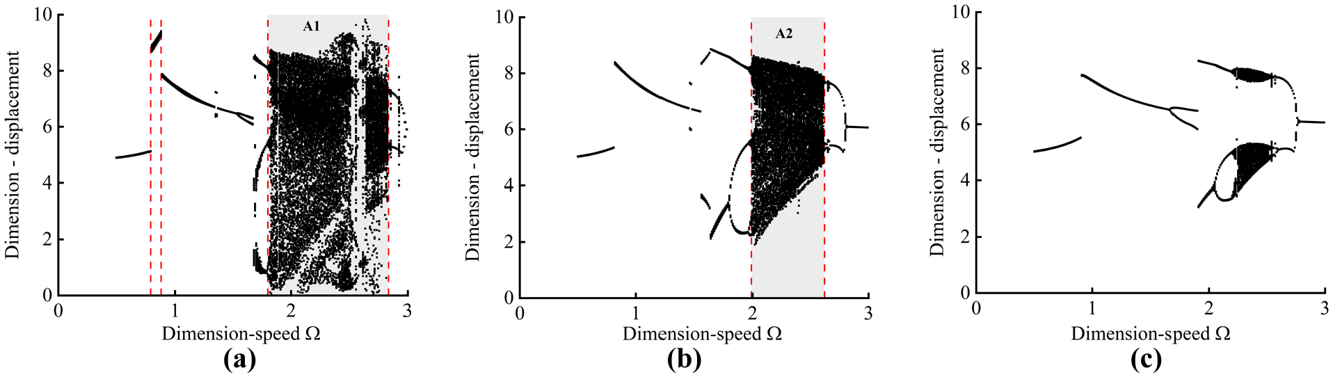
Bifurcation diagram of the system changing with dimensional speed under different friction coefficients: (a) μ = 0.0, (b) μ = 0.05, and (c) μ = 0.09.

From Figure 9(a), when Ω is in the [0.58,0.79] range, the system is one-periodic motion; when Ω is in the [0.79,0.88] range, the motion state of the system shows jumping phenomenon; when Ω increases to 1.63, the system bifurcates into two-periodic motion; when Ω increases to 1.72, the system bifurcates into three-periodic motion and multiple periodic motion; when Ω is in the [1.81,2.84] range, the system enters the chaotic motion state, and A1 is used to represent the chaotic region; when Ω continues to increase, the chaotic state of the system gradually weakens and the system enters the periodic state again.

From Figure 9(b), when Ω is in the [0.58,0.80] range, the system is one-periodic motion; when Ω increases to 0.81, the motion state of the system shows jumping phenomenon; when Ω increases to 1.63, the system bifurcates into two-periodic motion; when Ω increases to 1.83, the system bifurcates into three-periodic motion; when Ω is in the [1.99,2.62] range, the system enters the chaotic motion state, and A2 is used to represent the chaotic region; when Ω continues to increase, the system moves from chaotic state to 2-periodic state again and then finally stabilizes to 1-periodic state.

From Figure 9(c), when Ω is in [0.58,0.91], the system is one-periodic motion; when Ω increases to 0.92, the motion state of the system shows jumping phenomenon; when Ω increases to 1.68, the system bifurcates into two-periodic motion; when Ω is increased to 1.91, the two-periodic motion state of the system shows jumping phenomenon; when Ω increases to 2.12, the two-periodic motion of the system enters into three-periodic motion; when Ω is in the [2.42,2.69] range, the system will enter the chaotic motion state; when Ω continues to increase, the system moves from chaotic state to two-periodic state again, and then, it stabilizes to one-periodic state when Ω is equal to 2.81.

From Figure 9(a)–(c), with the increase in friction coefficient, the chaotic region gradually decreases, and the system exits from chaotic motion and returns to single periodic motion when the speed Ω = 2.62. When the speed is low (Ω < 1.8), the system has a stable motion state, and with the continuous increase in rotation speed, the chaotic characteristics of the system are obvious when there is no friction (μ = 0.0). With the increase in friction coefficient of tooth surface, the system drives the bifurcation inside the chaotic region by the bifurcation outside the chaotic region, and there is a short period of multiple periodic motions before entering the chaotic region. The increase in friction coefficient will increase the tooth surface resistance of the gear pair, and the area of the chaotic region will be significantly reduced.

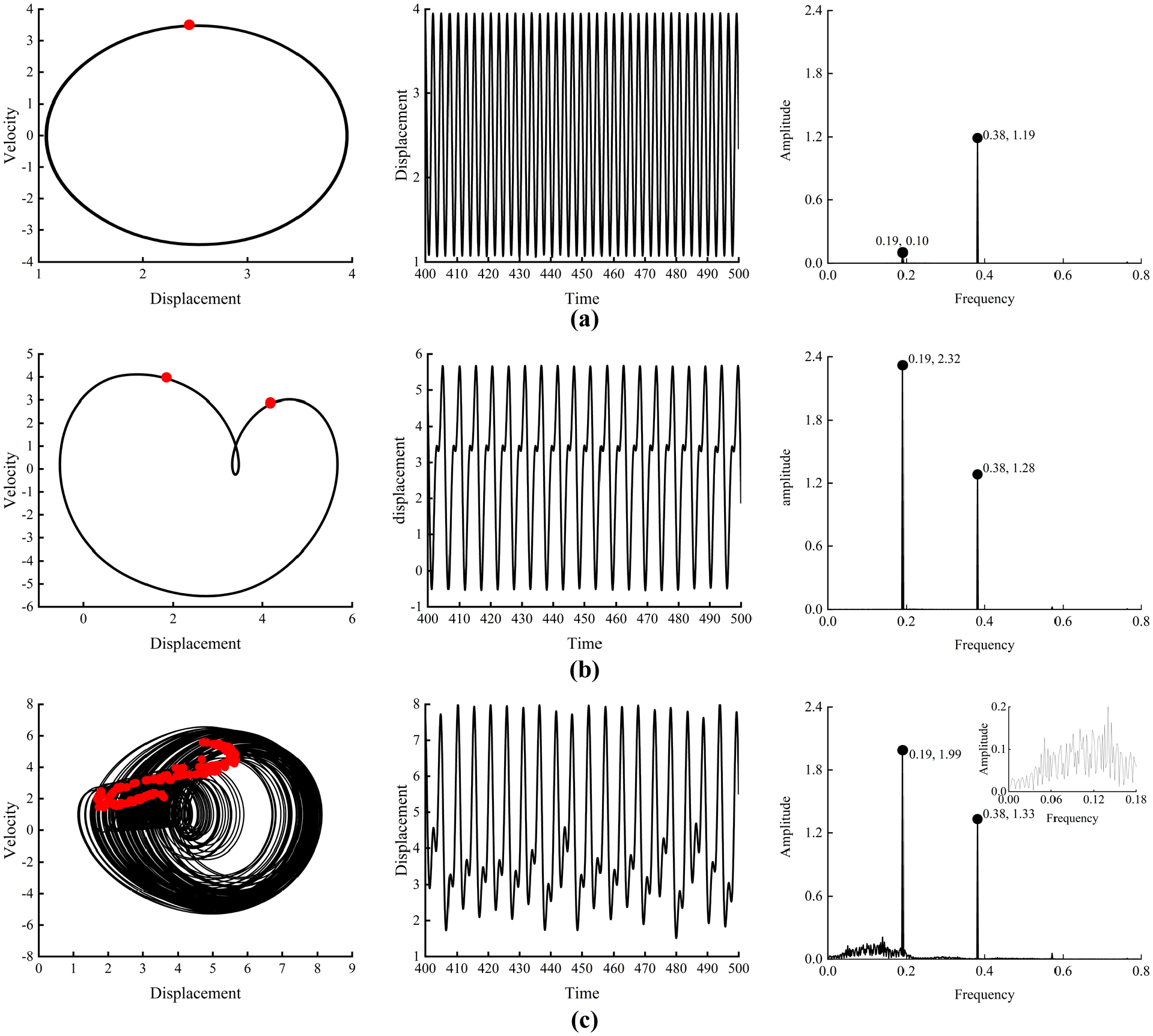
Figure 10 shows the phase diagram, Poincaré diagram, time history diagram, and spectrum diagram corresponding to the bifurcation characteristics at different rotating speeds when the friction coefficient is 0.05. The whole process of the system from one-period motion to chaos motion and then to one-period motion is analyzed. Here, the red solid dot represents Poincaré diagram.

Figure 10.

Phase, Poincaré, time history, and spectrum diagram with different dimensional speeds (Ω): (a) Ω = 1.00, (b) Ω = 1.79, (c) Ω = 1.96, (d) Ω = 2.00, (e) Ω = 2.61, and (f) Ω = 2.82.

Figure 10(a) shows that the system is in stable one-periodic motion. Figure 10(b) shows that when dimension speed Ω = 1.79, the frequency of bending vibration includes not only meshing frequency but also other continuous frequency components and the system enters aperiodic motion state. Figure 10(c) shows that when Ω = 1.96, the amplitude of the low-frequency region increases, indicating that the system is in an aperiodic motion state and tends to enter chaotic motion. In Figure 10(d), the ordered structure inside the phase diagram shows that the system is in quasi-periodic motion. Figure 10(e) shows that the sideband component appears near the meshing frequency, and the system enters into the chaotic motion state.

From Figure 10(a) to (e), the system moves from one-periodic motion to chaotic motion after multiple periods, and the phase diagram changes from regular circle to irregular shape and the Poincaré diagram gradually increases from the single vibration period point to the discrete multi-vibration period change. In the low-frequency part of fast-Fourier transform (FFT) spectrum, the amplitude of the system increases continuously, and the dynamic characteristics of the system become worse. Figure 10(e) and (f) shows that the system returns from chaotic motion to stable one-periodic motion state, the low-frequency amplitude of the system in FFT spectrum diagram decreases, and in Poincaré diagram, the range of vibration period number decreases gradually, and the dynamic characteristics of system are improved. The change in dynamic characteristics in Figure 10 is consistent with the performance of dynamic bifurcation characteristics in Figure 9.

Bifurcation characteristics of the system with the change in dynamic backlash

Take the dimension speed Ω equal to 2.4, the support clearance b_sx = b_sy = 10 μm, b_px = b_py = 10 μm, and the relative damping coefficient ζ = 0.05, the friction coefficient is 0.0, 0.05, and 0.09, respectively. The bifurcation diagram of the system dimension-relative displacement with the change in the backlash b_h is shown in Figure 11.

Figure 11.

Bifurcation diagram with dimension backlash under different friction coefficients: (a) μ = 0.0, (b) μ = 0.05, and (c) μ = 0.09.

From Figure 11(a), when b_h is in [0,3.72] range, the system is one-periodic motion; when b_h is equal to 3.73, the system bifurcates into two-periodic motion; when b_h is in [12.8,13.3] range, the system has multiple periodic motion and two-periodic motion; when b_h is increased to 13.4, the system enters into chaotic motion. From Figure 11(b), when b_h is in [0,3.61] range, the system is one-periodic; when b_h is equal to 3.62, the system bifurcates into two-periodic motion; when b_h continues to increase, the system experiences multiple periodic motion and then enters into chaotic motion. From Figure 11(c), when b_h is in [0,3.60] range, the system is one-periodic motion; when b_h is equal to 3.61, the system bifurcates into two-periodic motion; when b_h continues to increase, the system enters multiple periodic motion.

From Figure 11(a) to (b), the system moves from single-periodic motion to double-periodic motion and then enters chaotic motion through rapid change. The critical backlash does not change with the increase in friction coefficient. When the backlash is less than 4 μm, the system moves in single- periodic motion. When the backlash increases to 11 μm, the system suddenly enters chaotic motion. From Figure 11(b) and (c), the vibration amplitude changes little with the increase in backlash. With the increase in backlash, the system will produce irregular vibration due to the excessive backlash. The vibration amplitude will continuously increase with no tooth surface friction. With the increase in tooth surface friction, the chaotic region is divided from one block to three blocks. In order to avoid the chaotic movement of the system, the value of backlash should be in the range of 0–11.6 μm.

When the backlash changes from 2 to 16 μm, Figure 12 shows that the system moves from one-periodic motion to two-periodic motion and moves from the irregular vibration to chaos. From Figure 12(a) to (c), it is shown that in the low-frequency part of the FFT spectrum, the amplitude increases continuously, and the dynamic characteristics of the gear pair become worse. When the backlash b_h =16 μm, the FFT spectrum shows continuous other frequency components. Under the action of an unstable attractor, the system moves from period motion to chaos motion. It is also proved that the two-periodic motion is a way to enter chaos.

Figure 12.

Phase, Poincaré, time history, and spectrum diagram with different backlash (b_h): (a) b_h = 2 μm, (b) b_h = 11 μm, and (c) b_h = 16 μm.

Bifurcation characteristics of the system with the change in friction coefficient

When the dimension speed Ω = 2.4, the relative damping ratio is 0.05, 0.07, and 0.09, respectively. The bifurcation diagram of the system’s dimension relative displacement changing with the friction coefficient μ is shown in Figure 13.

Figure 13.

Bifurcation diagram with friction coefficient under different damping coefficients: (a) ζ = 0.05, (b) ζ = 0.07, and (c) ζ = 0.09.

From Figure 13(a), when the friction coefficient μ is in [0,0.43] range, the system is chaotic motion; when μ is in [0.43,0.69] range, the system includes two chaotic bands, which are accompanied by periodic motion and quasi-periodic motion; when the friction coefficient continues to increase, the system is stable in chaotic motion. From Figure 13(b), the main motion of the system is chaos motion. When the friction coefficient increases to 0.85, the system will be accompanied by periodic motion and quasi-periodic motion, and the state of chaos motion will be weakened. From Figure 13(c), when the friction coefficient is equal to 0.55, the system gradually changes from multi-period to three-period and finally stabilizes at two-period.

When the system dimension-rotational speed Ω = 2.4 and the relative damping ratio is 0.05, and the friction coefficient of the tooth surface changes from 0.46 to 0.69, the whole process of the system changing between chaotic motion and period doubling motion is shown in Figure 14. Figure 14(a) shows that the system is in chaotic motion state, and Figure 14(b) shows that under the action of stable attractor, the system changes from chaotic motion to periodic motion with the increase in friction coefficient of tooth surface and then enters into chaotic motion in the form of cataclysm. As shown in Figure 14(c), as the friction coefficient of tooth surface continues to increase, the system changes from the same cataclysm form and finally returns to the chaotic motion state. In the low-frequency part of FFT spectrum, with the primary and secondary changes in the three states of hybrid motion, periodic motion, and chaotic motion, the amplitude first increases and then decreases, and the dynamic characteristics of gear pair are in good and bad states.

Figure 14.

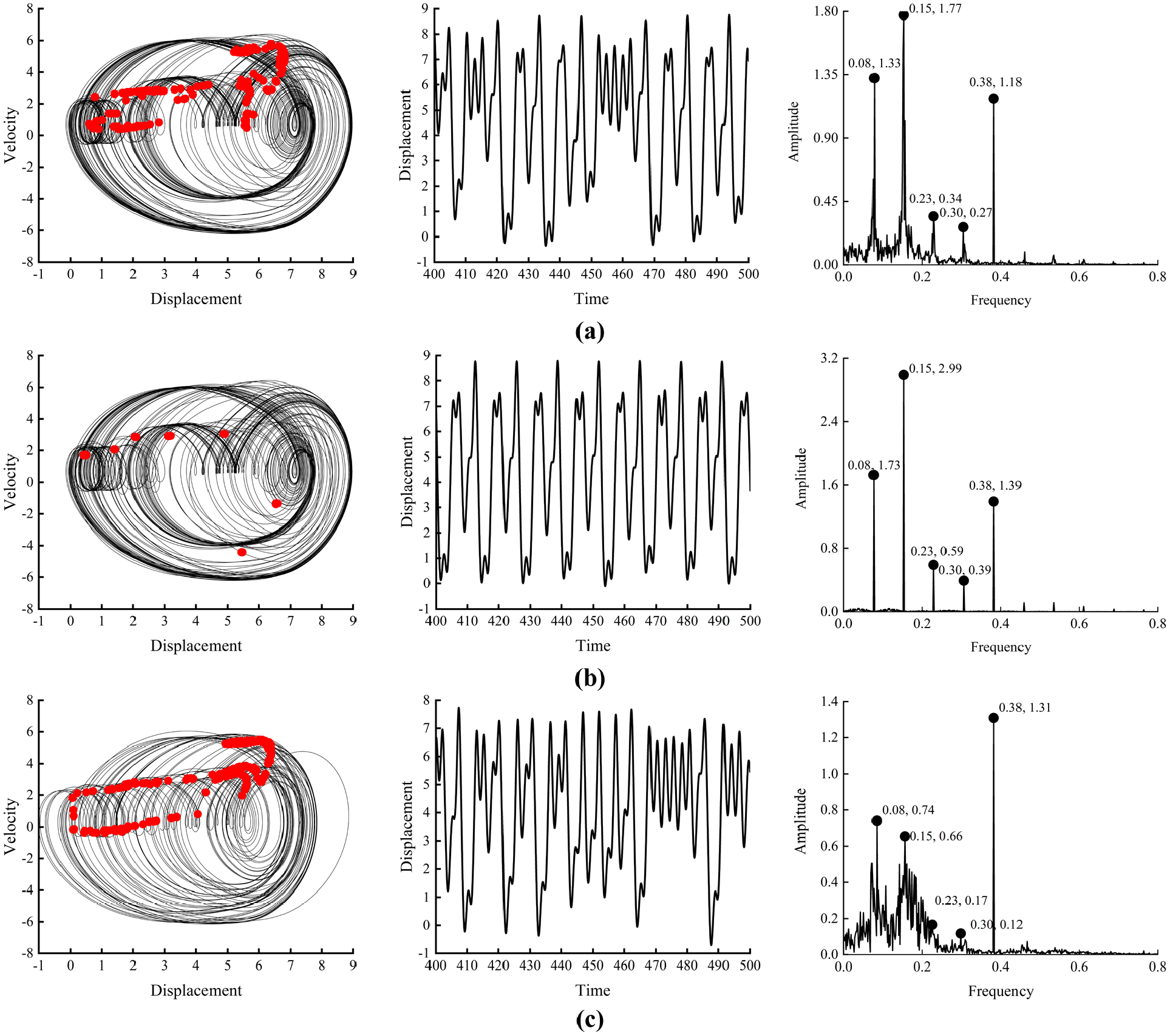
Phase, Poincaré, time history, and spectrum diagram with different friction coefficients: (a) μ = 0.46, (b) μ = 0.66, and (c) μ = 0.69.

Conclusion

In this article, a non-linear dynamic model of 6-DOF bending torsion coupling gear transmission system is established, which considers the time-varying friction coefficient of tooth surface, the time-varying mesh stiffness, and the fractal backlash. The bifurcation characteristics of the system are analyzed and studied under the influence of the parameters such as dimension speed, backlash, and friction coefficient of the tooth surface. The conclusions are as follows:

1. The innovation of this article is to introduce EHL theory and LTCA technology into the establishment of bending–torsion coupling non-linear vibration model of transmission system. The EHL model comprehensively consider the load distribution, the relative sliding velocity and rolling velocity of the tooth surface, the surface morphology of the gear, and the influence of lubrication conditions. EHL and LTCA methods are used to accurately obtain the friction coefficient and meshing stiffness of the time-varying tooth surface, which reflect the real meshing characteristics of the tooth surface from a micro-perspective and more accurately reflect the influence of various factors on the non-linear characteristics of the system. By using the fractal theory, dynamic backlash more accurately reflects the influence of the real tooth surface parameters on the non-linear bifurcation characteristics.

2. When the rotational speed changes independently, the chaos is obvious without the friction of the tooth surface. With the increase in tooth surface friction coefficient, the bifurcation behavior outside the chaotic region of the system will cause the bifurcation behavior inside the chaotic region, and the chaotic behavior of the system will be suppressed.

3. When the backlash changes independently, the vibration amplitude of the system increases continuously without tooth surface friction, and the non-linear characteristics of the system are obvious. With the increase in friction coefficient of tooth surface, the system gradually changes from chaotic behavior to quasi-periodic behavior and then to double-periodic behavior, which is suppressed. In order to avoid the chaotic movement of the system, it is very important to ensure the rationality of the backlash value. The value of backlash should be in the range of 0–11.6 μm.

4. When the tooth friction changes independently, with the increase in the tooth friction, the chaotic behavior of the system does not change significantly, and the vibration amplitude of the system decreases slightly. With the increase in damping coefficient, the tendency of regional partition of chaos behavior and the effect of chaos suppression are more significant.