Mesh-based tool path calculations for tubular joints

Abstract

Manufacturing of large steel tube structures is faced with excessive welding, fit-up and rework times in tube joints, due to various types of deviation from nominal shape of the tubes. This article presents a procedure and geometry calculus for generating cutting and welding paths based on measured geometries. The procedure poses the two measured meshes as per construction specification and invokes a mesh intersection procedure to get the mesh intersection path; performs an optional smoothing; interpolates the smoothed path to a specified angular resolution; estimates the two surface normal vectors and the two surface tangents in the plane spanned by the normals at each interpolation point; calculates the cutting tool and welding tool approach directions for obtaining the specified welding groove geometry at each interpolation point; and finally stores all the data parameterized by the interpolation angle. Illustrations of results with both synthetic, representative meshes and meshes obtained from scanning of actual tubes at the shop-floor at a manufacturer are presented. The reference implementation for the developed software tool is based on Python and uses the mesh modeller from the 3D creation suite Blender as platform.

Introduction

Large steel tube structures, such as offshore jackets, are truss geometries composed of legs of larger diameter and braces of smaller diameter tubes; these are names of the offshore jacket terminology. ¹ The manufacturing of these requires cutting and joining, which is typically performed by a plasma or oxy-fuel cutting process and an arc welding process, respectively. Bracing stubs are saddle-cut to fit at particular angles and transversal offsets in complex joints on the leg tubes. The bracings are then butt welded in the field between bracing stubs on different legs.

Saddle cutting of tubes is probably as old a trade as tube and pipe constructions. The first generic saddle cutting machine was invented by Dwight ² in 1933. It takes into account the diameters of the tubes, as well as the orthogonal offset and the angle between the axes of the two cylinders. Later Smith ³ claims to be the first to invent a field-portable saddle cutter, which, however, only considers cuts in cylinders with axes at a right angle. Contemporary shop-floor cutting of large tubes is generally performed by commercially available computer numerical control (CNC) plasma cutters.

The fabrication of steel tubes is possible only up to a certain accuracy. Steel tubes for large offshore structures are allowed certain tolerances according to a standard, for example, NORSOK M-101. ⁴ This particular standard defines and allows for tolerances in four relevant types of deviations: circumference, roundness, circularity and straightness. The tolerances in the standard lead us to a rough estimation of the worst case of the extra weld volume to fill. This we have estimated at some 50% for a representative geometry; that is, realistic tube radii, joint angle, wall thickness and so on. Industrial partners have calculated that poor geometric fitting in saddle cuts, presumably due to deviation from nominal tube geometry, causes approximately 25% extra welding time and material. In addition to this approximately 40% extra fit-up and rework time is calculated for the same reasons. Fit-up is the operation of placing a stub on a leg to the design reference within design tolerance by means of a global metrology system. Rework is the operation of field-grinding the saddle-cut to eliminate large gaps in the fit. A rework operation thus entails one extra fit-up operation.

To the best of our knowledge, it is the nominal geometry of the tubes, which is generally used for calculating the saddle curve of cutting in the CNC cutter path generation software. Obviously, zero order correction to the nominal geometry, obtained by measurement and fitting the radius of the tubes, can be trivially incorporated when specifying a cutting task to the path generation software. Cylinders are quadric surfaces in 3D and their intersection curve may be derived and parameterized.^5,6 In fact, the most general quadric surface that would be desirable to make a fit to, based on measurement of the pertinent tubes, would be an ellipsoid. However, everything beyond zero order corrections to the nominal geometry, that is, corrections to the radii of the tubes, would require handling of reference data, for example, axis position and azimuth, on the tubes, which would complicate the cutting machine interface and further handling of the cut tube. The speculative assumption presented here is that shop-floors utilizing contemporary CNC machines for tube cutting at most incorporate zero order corrections to the tube radii, and that contemporary CNC cutters do not support any further corrections.

It is uncertain whether a quadric approximation to the tube surfaces will be sufficient for a good saddle cut. It could be argued that it is mainly eccentricity which makes up the deviation in the tubes, and hence a quadric fit to the actual geometry would in principle be perfect. However, particularly welded steel tubes, that is, steel tubes formed by rolling and closing of a plate with a weld, will exhibit some considerable deviation from circular cross section in a neighbourhood of the closing weld, where it appears as two flat surfaces meet in the weld, an effect known as peaking. Palumbo and Tricarico ⁷ showed that the peaking in uncalibrated steel tubes can be considerable. If peaking is dominating over the eccentricity in the deviation of the tubes, the tube shapes cannot be fitted well by quadric surfaces, and other modelling methods must be applied.

An obvious candidate for modelling the peaking of welded steel tube cross sections would be the use of ruled surfaces for fitting to measurements to the actual geometries on the shop-floor. With an adequate set of metrological measurements of a cross section at the joint positions of the tubes, it is trivial to approximate the tubes in the joint regions by ruled surfaces. With further cross-sectional measurements along the axes of the tubes, conical elements may be added to the fitting ruled surfaces. The intersection curve of two developed ruled surfaces is well described by Heo et al. ⁸ By extensive measurements in the neighbourhoods of the joint, this may be extended to take longitudinal variations into account by considering piecewise, developed ruled surfaces.

Once on the path of extensive metrological measurement it is tempting to go all the way and use a modern, metrologically adequate point cloud capturing system for creating a mesh map of the neighbourhoods in question. Reliable algorithms exist for finding the intersection mesh curve, which arises as the intersection of two mesh surfaces. ⁹ Elsheikh and Elsheikh ¹⁰ further developed such algorithms with respect to degenerate cases and optimization. Laser profile scanners, which can be described as 1D-based point cloud capturing systems, with accuracy in the order of $10\mu m$ have been available for some decades, and find their use in diverse industries, for example, for mapping items on conveyors in goods and food manufacturing, and for groove mapping and tracking in arc welding. An example of such a laser profile scanners is the ‘scanCONTROL 2900-100’ from Micro-Epsilon.

The past decade has seen an immense development in both proper, that is, 2D-based, point cloud capturing systems and software tools for handling and analysing the large amount of data in sampled point clouds. Modern point cloud capturing systems are available and provide point clouds with a resolution of $~1\mathrm{mm}$ and with an internal accuracy of $<<1\mathrm{mm}$ . Examples of mobile point cloud capturing systems, suitable for mounting on a robot for volume coverage, are the ‘HandySCAN 3D’ from Creaform, the ‘MetraSCAN 3D’ system from Creaform, the ‘Freestyle3D X’ from Faro and the ‘One’ from Zivid. It should be noted that the Zivid ‘One’ may be considered inadequate for the geometric scale of the particular application addressed in this article.

Particularly interesting for the topic in this article are devices and software which may register the captured point clouds of a tube surface region to a topologically sound, and accurate mesh surface of the tube neighbourhoods relevant for the joint. The fundamental techniques for triangulating ¹¹ and registering ¹² point clouds to meshes have been known for some decades. When such internally accurate meshes of regions of the tubes can be related, by other metrological means, to the references of the tube geometries, this opens an opportunity for calculating cutting paths on a discretization of the actual tube geometries at the joint, as opposed to fitting to approximate, parametric models.

Robotized installations exist for densely measuring and cutting to actual tube geometry. Such installations are available from companies Kranendonk Production Systems BV and Ingenieurtechnik und Maschinenbau GmbH. However, it is expected that many sites working with large-scale steel tube constructions already have working CNC cutters, methods for measuring and fit-up, automated or welding installations and transportation systems for large tubes and structures, as well space allocated on the shop-floor with associated routines for all operations. Switching to an integrated installation covering all these aspects of operations is not an easy transition, neither regarding equipment investment nor regarding implementation and internal and external certification procedures.

The presented article focuses on the means of generating a tool path for the CNC cutter for the saddle of the branch stubs, which will be possible to integrate with the equipment in an existing manufacturing system. Two major aspects are not thoroughly treated in this article.

First, the point cloud capturing system and metrology system together must ensure the establishment of a sufficiently accurate mesh with sufficiently correct reference to the tube geometry for both leg and branch tubes. This must be addressed during introduction of the point cloud capturing system. It is already known that some point cloud capturing systems are available with software for triangulation of the point clouds into meshes; for example, the ‘SCENE’ software suite from Faro and the included capturing software for the Creaform ‘HandySCAN 3D’.

Second, the method for establishing correspondence between the captured geometry and the tube references will be depending on the capturing system set-up and its ability to integrate its reference with other metrology systems already on the shop-floor. An isolated mechanism might be to add markers at known locations on the tube in the neighbourhood of the joint, and then ensure that the point cloud of the tube includes these markers. Thus independent analysis of the point cloud will be able to establish the correspondence to the tube reference by only knowing the location of the markers in the reference.

Third, a means of executing the calculated cutting path for the branch stub saddle with reference to the actual tube geometry is the CNC cutting machine. One technique would be to take over the high level control of the CNC machine, feeding a trajectory which traces the cutting path and controlling the tool in synchronicity with the trajectory. It is highly unlikely that this technique will be possible on contemporary CNC cutters on shop-floors. Another technique will be to express the cutting path into a format which the CNC cutter can load, for example, G-code. Even though this is a fairly standard way of executing tasks on CNC machines, it is uncertain whether CNC cutters for tubes generally allow such low level interfacing. The last resort is to replace the CNC cutter with a long-reaching industrial robot equipped with a cutting tool. The robot will certainly be able to execute a free tool path.

The focus on adapted cutting path generation is due to the consequence, that is, excess time and material in welding the joint. The welding process is generally manual, and the welders weld whatever groove they observe. However, for the sake of future automated welding, it will be adequate to utilize the detailed saddle curve also for the generation of the welding tool path. We include this as a by-product of the geometry calculation.

The remainder of this article is dedicated to describing the principles and prototype software system for calculation a cutting path and an associated root weld path for a tube y- or t-connection with any angle or off-axis offset. Section ‘Principle of solution’ describes the concepts and remedies which will solve the problem. Section ‘Prototype implementation and results’ describes a prototypical, but working, implementation, and illustrates and discusses the obtained results. Section ‘Conclusion and discussion’ contains conclusion and discussion.

Principle of solution

We assume that two tubes for leg and stub are given; denoted by $\mathfrak{l}$ and $\mathfrak{s}$ , respectively. The tubes are defined in reference frames $\mathcal{L}$ and $\mathcal{S}$ respectively. The tool task path for the CNC cutting process is to be calculated with respect to the stub reference, since the saddle cutting is performed on the stub.

The adapted saddle cutting problem may arise with tubes of any dimensional scale, but the following dimensions give an indication of the pertinent case at hand.

The leg tube is typically several tens of metres long while the branch stub tube protrudes a couple of metres from the leg surface. Leg and branch tubes are specified by their outer diameter or radii, ${r^o}_{\mathfrak{l}}$ and ${r^o}_{\mathfrak{s}}$ respectively, where ${r^o}_{\mathfrak{l}}>{r^o}_{\mathfrak{s}}$ . The leg tube diameter is typically of the order of $2m$ , that is, $r_{\mathfrak{l}}=1m$ , and the branch tube diameter is typically of the order of $1m$ , that is, $r_{\mathfrak{s}}=0.5m$ . The wall thicknesses of the tubes, $d_{\mathfrak{l}}$ and $d_{\mathfrak{s}}$ , are in the range of several tens of millimetres, with $d_{\mathfrak{l}}~50\mathrm{mm}$ being common.

When welding a stub on a leg, a weld groove must be cut to a varying groove angle around the cut contour of the stub-end. Typically welding is done from the outside, which means that the groove opens from the inner stub surface towards the outer stub surface. Depending on wall thicknesses, tube diameters and pitch of the joint, in some set-ups both inside and outside welding will occur. In these situations, there will typically be a pure outside groove at the toe and a pure inside groove at the heel, with a mixed groove at some changeover segment between toe and heel. We will, for simplicity, assume a pure outside groove. Hence, the interesting intersection curve between the leg and stub is found between the outer surface of the leg and the inner surface of the stub.

The leg tube as a whole has a global reference system, but for each stub joint a particular reference system is introduced, which is called the working reference for the particular stub. The pertinent working reference for the leg tube is denoted by $\mathcal{L}$ Both tubes are located with their axes along their respective $\hat{z}$ s and their origos on their respective axes. The origo of the leg tube lies on the leg axis, at the closest location to the stub axis. The leg tube has ${\hat{x}}_{\mathfrak{l}}$ in the plane spanned by ${\hat{z}}_{\mathfrak{l}}$ and ${\hat{z}}_{\mathfrak{s}}$ , and the stub tube has ${\hat{x}}_{\mathfrak{s}}$ pointing in the projected direction of the toe of the saddle, that is, mainly away from the leg tube. The origo of the stub tube is placed at the distal end of the stub, from the tube joint. The stub $\hat{z}$ is pointed towards the leg tube. The leg ${\hat{z}}_{\mathfrak{l}}$ is chosen with positive projection on the stub ${\hat{z}}_{\mathfrak{s}}$ .

Under these definitions, the stub tube pose may be described constructively by first aligning the two references, then rotating the stub by its pitch, $\theta$ , around $-\hat{y}$ , then translating it by its offset, $\delta$ , along $\hat{y}{\prime }_{\mathfrak{s}}$ , and finally displacing it by its protrusion, $\mathrm{\Delta }$ , along the $-\hat{z}\prime$ , all in mobile coordinates indicated by the primes. The resulting coordinate transform places $\mathcal{S}$ with respect to $\mathcal{L}$ , and is denoted by ${\mathcal{S}}^{\mathcal{L}}$ .

From the measurement system we obtain the captured meshes of the relevant regions of the outer leg surface and the inner stub surface. We denote these meshes by $\mathfrak{L}$ and $\mathfrak{G}$ , respectively. We further assume that the surface measurement system is either integrated with the on-site metrology system, or that post-processing of the measured surfaces is possible, such that the meshes can be formulated in their relevant references, that is, such that we are given ${}^{\mathcal{L}}\mathfrak{L}{}^{\mathcal{S}}\mathfrak{G}$ .

We require that these meshes be well-formed, that is, that they locally describe a surface without degeneracies. We further require $\mathfrak{G}$ that is topologically isomorphic with a finite cylinder surface and that $\mathfrak{L}$ is topologically isomorphic with a disc in 3D. Thus $\mathfrak{G}$ will have two closed boundary curves and $\mathfrak{L}$ will have one closed boundary curve.

To perform mesh operations the meshes must be formulated with the same reference. Since the cutting process must refer to the stub reference, all mesh computation will be performed with respect to $\mathcal{S}$ . Hence we use the known stub pose on the leg working coordinates, ${}^{\mathcal{L}}\mathcal{S}$ , to formulate its inverse, ${}^{\mathcal{S}}\mathcal{L}={}^{\mathcal{L}}{\mathcal{S}}^{-1}$ , with which we can transform the leg mesh: ${}^{\mathcal{S}}\mathfrak{L}={}^{\mathcal{S}}\mathcal{L}{}^{\mathcal{L}}\mathfrak{L}$ . We will assume all geometry henceforth to be expressed in stub reference.

Mesh intersection generation

We now suppose that we have available some mesh intersection algorithm, such as the first part of the algorithm described by Lo. ⁹ That is, the meshes are topologically correct, sampled with sufficient coverage of the intersection region, and posed correctly according to a possible structural configuration. Under these circumstances, the intersection will be a topological correct mesh curve tracing a closed path. Figure 2 illustrates two tube meshes with the intersection calculated by an intersection algorithm. The highlighted vertices and edges are the intersection curve, which is returned by the algorithm.

The result of the mesh intersection algorithm is a mesh with no faces, which describes a closed curve and is topologically isomorphic with the boundary of a disc in 3D.

Let $\mathfrak{X}$ denote the intersection mesh and let $\{V^{\mathfrak{X}},E^{\mathfrak{X}}\}$ denote the direct sets of vertices and edges in $\mathfrak{X}$ ; that is, the vertices and edges highlighted in Figure 2. The vertices in $V^{\mathfrak{X}}$ are, being elements of a mesh, not listed in any particular order, and their topological information is carried by the linking edges in $E^{\mathfrak{X}}$ . This latter statement is not true for all mesh data structures, but it is a safe assumption since it puts no requirement on the finally chosen format of the data structure.

If $\mathfrak{X}$ is to describe a simple, closed intersection curve, we may check that the vertices and edges indeed describe such a structure. It may be assumed that the mesh data structure returned by the mesh intersection algorithm is consistent and not inherently degenerate.

For describing the requirements on $\mathfrak{X}$ , we use the standard graph functions $V$ and $E$ . $V$ returns the pair of vertices connected by a given edge and $E$ returns the set edges that connect to a given vertex. We further use the function $C$ , which returns the 3D coordinates of a given vertex. The requirements on $\mathfrak{X}$ to be correct may thus be formulated as

$$\forall v\in V^{\mathfrak{X}}:|E(v)|=2(\mathrm{closedcurve})$$

(1a)

$$\forall e\in E^{\mathfrak{X}}:V(e)\subset V^{\mathfrak{X}}(\mathrm{closedness})$$

(1b)

$$\forall e\in E^{\mathfrak{X}},\exists v\in V^{\mathfrak{X}}:e\in E(v)(\mathrm{coverage})$$

(1c)

$$\forall e\in E^{\mathfrak{X}}:(v,v\prime )=V(e)\Rightarrow v\ne v\prime (\mathrm{non}-\mathrm{degeneracy})$$

(1d)

$$\forall v\in V^{\mathfrak{X}}:E(v)\subset E^{\mathfrak{X}}(\mathrm{closedness})$$

(1e)

$$\forall v\in V^{\mathfrak{X}},\exists e\in E^{\mathfrak{X}}:v\in V(e)(\mathrm{coverage})$$

(1f)

$$\forall v\in V^{\mathfrak{X}}:e=(v,v\prime )\in E(v)\Rightarrow e\in E(v\prime )(\mathrm{reciprocity})$$

(1g)

$$\forall v,v\prime \in V^{\mathfrak{X}}:C(v)=C(v\prime )\Rightarrow v=v\prime (\mathrm{uniqueness})$$

(1h)

$$\begin{array}{c}\multicolumn{1}{c}{\forall e,e\prime \in E^{\mathfrak{X}}:e=\{v,v\prime \}\wedge e\prime =\{v,v\prime \}\Rightarrow e=e\prime }\\ \multicolumn{1}{c}{(\mathrm{uniqueness})}\end{array}$$

(1i)

A couple of post-processing steps is required to obtain a set of path data adequate for generating smooth tool trajectories for cutting and welding the joint. The post-processing steps comprise the following:

1. Serialization of $V^{\mathfrak{X}}$ to a path of positions, where $E^{\mathfrak{X}}$ is used to determine the sequence and $C$ is used to extract vertex position.

2. Uniform re-sampling by linear interpolation in the stub azimuth over the intersection path.

3. Smoothing using a cubic B-spline.

Path generation

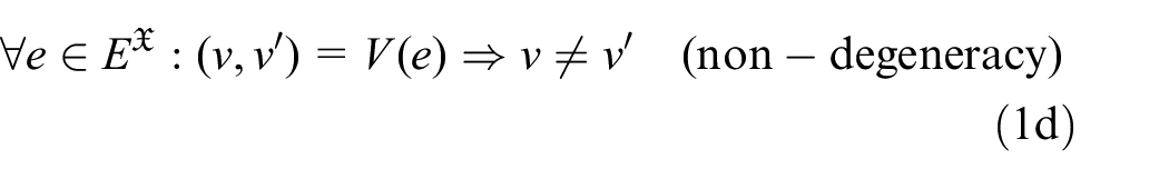
Topologically, for the mesh to form a simple, closed intersection curve, it is a necessary condition that all vertices have exactly two connecting edges, as noted in equation (1a). A sufficient condition is that starting from any vertex, initially selecting one arbitrary edge from that vertex, and then following the non-traced edges to new vertices, will end up tracing all vertices and edges exactly once. We further require that if the curve is projected onto the ${\hat{x}}_{\mathfrak{s}}-{\hat{y}}_{\mathfrak{s}}$ -plane it must make up a Jordan curve; that is, the projected curve must be non-self-intersecting.

Provided that this precondition is fulfilled, the first post-processing step is to organize the vertices in topological sequence. A natural parameter for ordering the vertices on the stub tube is the azimuth angle of cylindrical coordinates in Euclidean space, ${\mathit{E}}^3$ . We choose a stub azimuth function onto a specific parameterization of the unit circle, $S^1$ : ${\varphi }_{\mathfrak{s}}:{\mathit{E}}^3\to [0\mathrm{rad};2\pi \mathrm{rad}[,$ measuring the azimuth in stub reference from $\hat{x}$ and with $\hat{z}$ as positive rotation vector. Effectively ${\varphi }_{\mathfrak{s}}$ is defined on the domain ${\mathit{E}}^2$ in the ${\hat{x}}_{\mathfrak{s}}-{\hat{y}}_{\mathfrak{s}}$ -plane.

This may be used for topological ordering of the vertices in $V^{\mathfrak{X}}$ , provided that the measured geometries and the measurement disturbances combined stay within tolerances that the two connected vertices for any vertex has azimuth lower and higher than the vertex itself.

We may establish a mapping from the set of vertices, using the edges, to provide the connected vertices $c:V^{\mathfrak{X}}\to V^{\mathfrak{X}}\times V^{\mathfrak{X}}$ . Further, to trace the vertices in a particular direction with respect to $\hat{z}$ , we need an indication to distinguish the rotation direction of the two connected vertices with respect to their common neighbour. Technically this may be achieved by defining a rotation direction indicator function between two ordered vertices, determining whether rotation is aligned or counter-aligned with $\hat{z}:{\mathcal{X}}_{{\varphi }_{\mathfrak{s}}}(v,v\prime )=\mathrm{sgn}(\hat{z}·(v\times v\prime ))$ . Note that ${\chi }_{{\varphi }_{\mathfrak{s}}}$ cannot simply be defined as the difference in azimuth, due to the cyclic nature of $\mathrm{SO}(2)$ and its algebra $\mathfrak{s}\mathfrak{o}(2)$ .

Algorithm 1 shows the ordering according to azimuth of the vertices. $P^{x_o}$ here denotes a finite sequence, and a subset of ${\mathit{E}}^3$ , containing the coordinates of all the vertices in $V^{\mathfrak{X}}$ , $P^{x_o}=({\mathbf{p}}_i)$ ; where the reference to $\mathcal{S}$ is implied. The algorithm ensures that $P^{x_o}$ is well-ordered with respect to ${\varphi }_{\mathfrak{s}}$ ; that is, $\forall i:{\varphi }_{\mathfrak{s}}({\mathbf{p}}_{i+1})>{\varphi }_{\mathfrak{s}}({\mathbf{p}}_i)$ .

Algorithm 1 Azimuth ordering algorithm

1: function AZIMUTH ORDERED PATH( $V^{\mathfrak{X}}$ , $E^{\mathfrak{X}}$ ) 2:   $P^{x_o}\leftarrow \mathrm{new}\_\mathrm{list}()$ 3:   $v_{\mathrm{toe}}\leftarrow \underset{{\varphi }_{\mathfrak{s}}}{min}\{V^{\mathfrak{X}}\}$ 4:   $v_{\mathrm{last}}\leftarrow v_{\mathrm{toe}}$ 5:   $P^{x_o}.\mathrm{append}(\mathrm{coords}(v_{\mathrm{last}}))$ 6:   $v_{\mathrm{cur}}\leftarrow {\underset{{\mathcal{X}}_{{\varphi }_{\mathfrak{s}}}}{max}}_{(v_{\mathrm{last}},·)}\{c(v_{\mathrm{last}}\}$ 7:  While $v_{\mathrm{cur}}\ne v_{\mathrm{toe}}$ do 8:    $P^{x_o}.\mathrm{append}(\mathrm{coords}(v_{\mathrm{cur}}))$ 9:    $v_{\mathrm{last}}\leftarrow v_{\mathrm{cur}}$ 10:    $v_{\mathrm{cur}}\leftarrow {\underset{{\mathcal{X}}_{{\varphi }_{\mathfrak{s}}}}{max}}_{(v_{\mathrm{last}})}\{c(v_{\mathrm{last}})\}$ 11:  End while 12:  return $P^{x_o}$ 13: end function

The path positions in $P^{x_o}$ may be strongly irregularly distributed in the azimuth domain, that is, the sequence of azimuth angles of the intersection path, ${\mathrm{\Phi }}^o=({\varphi }_{\mathfrak{s}}({\mathbf{p}}_i))$ . This, of course, depends on the meshes generated by the measurement system in terms of measurement grid irregularity, surface variations and measurement noise.

To ensure a uniform sampling a second post-processing step is performed, consisting of a piecewise linear interpolation, which is run through the points in $P^{x_o}$ , using the azimuth function ${\varphi }_{\mathfrak{s}}$ over the coordinates as parameter. The azimuth-based ordering of $P^{x_o}$ ensures that the piecewise linear interpolation and ensuing sub-sampling are straightforward. We define the closed linear interpolator $L_{{\mathrm{\Phi }}^o,P^{x_o}}:[0\mathrm{rad};2\pi \mathrm{rad}[\to {\mathbf{E}}^3$ , where extrapolation at the boundary at $2\pi \mathrm{rad}$ is done by cyclic conditions.

Based on the desired resolution of the final cutting and welding trajectories, an azimuth resolution, $\delta \varphi$ , should be determined. An equidistant set of interpolation angles is formed as

$${\mathrm{\Phi }}^l={({\varphi }_i=i\delta \varphi )}_{i=0}^{i\delta \varphi <2\pi \mathrm{rad}}$$

(2)

Sampling $L_{{\mathrm{\Phi }}^o,P^{x_o}}$ with the azimuth basis ${\mathrm{\Phi }}^l$ gives us the interpolated path as the sequence $P^{x_l}={(L_{{\mathrm{\Phi }}^l,P^{x_o}}(\varphi ))}_{\varphi \in {\mathrm{\Phi }}^l}$ .

The last step addresses the need for being able to generate a smooth, finely interpolated path suitable for executing on the CNC tube cutter and on the welding robot. For this, a cubic smoothing spline is run over the interpolated path. Ideally the spline data is stored and transferred for pre-processing before the CNC tube cutter and the welding processes, thus interpolating to the correct coarseness for the pertinent processes.

Let $B_{{\mathrm{\Phi }}^l,P{x}_l,s}:[0\mathrm{rad};2\pi \mathrm{rad}[\to {\mathit{E}}^3$ denote the closed cubic B-spline over the parameters ${\mathrm{\Phi }}^l$ of the interpolated path points $P^{x_l}$ with smoothing parameter $s$ . For illustrations and task path generation we will denote the sampled, smoothed spline path by $P^{x_s}$ , generated by sampling $B_{{\mathrm{\Phi }}^l,P^{x_l},s}$ with ${\mathrm{\Phi }}^s={\mathrm{\Phi }}^l$ . Thus the sequence of the smoothed path is $P^{x_s}={(B_{{\mathrm{\Phi }}^l,P^{x_l},s}({\varphi }_i))}_{{\varphi }_i\in {\mathrm{\Phi }}^s}$ .

The process of smoothing will not be further detailed here, since it is considered a part of the tool process preparation rather than task generation. If $P^{x_l}$ is stored as the result of the task generation process then, at any later stage, the smoothing and fine interpolation can be suitably performed for the pertinent tool process. We will use the smoothing spline step mainly for visualization purposes in the following.

Surface normal vectors generation

The smooth path in $P^{x_s}$ merely describes the intersection of the inner stub tube surface with the outer leg tube surface at the joint to be formed. It is not in itself a task description, but only an important underlay for generating cutting and welding tasks in the simple case of pure outside welds.

Another set of important, geometric underlays for task generation are the leg and stub normal vectors at the path points in $P^{x_s}$ . Let $N_s$ and $N_l$ denote these sequences, respectively. These are important, since they represent, to the first order, the local geometry at the path points. Notably the leg tube normal vectors are important, since it is from the local leg surface that the groove opening angle and hence the cutting tool direction is to be counted. Likewise with the weld tool approach direction $N_s$ may be important for determining tool access conditions for the welding tool in the heel region of the tube joint.

We could utilize an average of the mesh face normal vectors in the neighbourhood of a path point, if those are available in the mesh format given by the measurement system. This would probably require the least computational load. However, the face normal vectors may not be represented or readily accessible in the given mesh format. Hence it is better to base the normal estimation on a cloud of mesh vertices in a neighbourhood of the path point, since the position of vertices presumably are readily accessible for any mesh format.

The selection and extraction of neighbour vertices are easily done by the use of k-d trees over the positions of vertices in $\mathfrak{G}$ and $\mathfrak{L}$ . ¹³ Let $K^{\mathfrak{s}}$ and $K^{\mathfrak{l}}$ represent the k-d trees over all vertex points in the meshes $\mathfrak{G}$ and $\mathfrak{L}$ , respectively. Then for each path position, ${\mathrm{p}}_i\in P^{x_s}$ , each of the k-d trees is queried to get a set of $k$ nearest neighbour positions from the two meshes, ${\left\{{\mathbf{n}}_{i,j}\right\}}_{j<k}=K^{\mathfrak{s}}({\mathbf{p}}_i,k)$ and ${\left\{{\mathbf{n}}_{i,j}\right\}}_{j<k}=K^{\mathfrak{l}}({\mathbf{p}}_i,k)$ . We have assumed that a suitable, universal number of neighbours, $k$ , is feasible. Generally, a more analytical approach for each location in the meshes should be used for generating region-dependent, suitable numbers of neighbours, $k_{{\mathfrak{s}}_i}$ and $k_{\mathfrak{l}i}$ , for every path point p _i . Each set of neighbours are used for computing estimates, ${\hat{n}}_i^{\mathfrak{l}}$ and ${\hat{n}}_i^{\mathfrak{s}}$ , of the surface normal vectors for the actual geometries at p _i .

The topic of stable and true normal estimation from point clouds have been studied extensively in recent decades due to the advance in the technology of point cloud capturing systems. A direct, local technique over a neighbourhood of the point of estimate, as well as considerations about the size of neighbourhood to choose, is described by Mitra and Nguyen. ¹⁴ We will proceed with the presumptions that the small curvature of the tubes, relatively weak variation in the tube surface details and the relatively low noise of the capturing technology do not impose us with detailed considerations over the size of neighbourhood for stable and true normal estimation. In other words, we expect that we may choose a conservatively large neighbourhood in the tube meshes at a path point for normal estimation.

Consider a neighbourhood around path position p _i of $k$ points of either the stub or the leg mesh. Let N ⁱ denote the $3\times k$ array obtained by horizontally stacking the column vectors for the $k$ selected neighbourhood points in $\{n_{i,j}{\}}_j$ . Then the estimated surface normal direction, ${\hat{n}}_i$ , is found by choosing the eigenvector of lowest eigenvalue of the auto-covariance matrix $\mathrm{cov}({\mathbf{N}}^i)$ . In practice we utilize the fact that since $\mathrm{cov}({\mathrm{N}}^i)\propto {\mathrm{N}}^i{{\mathrm{N}}^i}^T$ , the eigenvectors of the latter have the same directions as those of the former, and the eigenvalues keep their relative ordering. This minimum-eigenvector must then be normalized and possibly reversed in direction to denote the appropriate inwards or outwards normal of the surface, ${\hat{n}}_i$ , at p _i .

For task generation, the most interesting normal vectors are the outwards normal vectors of the leg and stub outside surfaces. It is these we denote by the sequences $N={\left({\hat{n}}_i^{\mathfrak{l}}\right)}_i$ and $N_{\mathfrak{s}}={\left({\hat{n}}_i^{\mathfrak{s}}\right)}_i$ .

Another interesting local feature to evaluate over the interpolation base is the path tangent in a right-hand positive traversing manner, according to the stub z-direction, ${\hat{z}}^{\mathfrak{s}}$ . It is calculated as proportional to the cross product of the stub and leg normal vectors, in that order, and normalizing appropriately

$$\hat{t}\propto {\hat{n}}^{\mathfrak{s}}\times {\hat{n}}^{\mathfrak{l}}$$

(3)

The sequence of path tangents is denoted by $T={\left({\hat{t}}_i\right)}_i$ .

The general result of the geometry analysis for a given desired interpolation basis is the sequence of quintuplets

$$\{{\mathrm{\Phi }}^l,P^{x_s},T,N,N\}={({\varphi }_i,{\mathbf{p}}_i^{x_s},{\hat{t}}_i,{\hat{n}}_i^{\mathfrak{s}},{\hat{n}}_i^{\mathfrak{l}})}_i$$

(4)

Task path generation

The detailed calculations for the pertinent tool operations of cutting and welding must be done with knowledge about the particular tube material, tube thicknesses, tool processes, machinery and software interfaces that are to be used to perform them. However, simply using the surface normal vector sequences of the leg, $N_{\mathfrak{l}}$ , and stub, $N_{\mathfrak{s}}$ , together with a minimum of joint groove geometry specification, allows us to calculate tool approach directions and tool centre positions along the joint intersection path $P^{x_s}$ ; that is, the purely geometrical parts of the tool operations.

Let $\{{\mathrm{\Phi }}^{c_0},A^{c_0}\}$ denote the sequences ${({\varphi }_i^{c_0},{\alpha }_i^{c_0})}_{i<n^{c_0}}$ which specifies $n^{c_0}$ pairs of desired joint groove opening angle, ${\alpha }^c$ , at certain stub tube azimuths, ${\varphi }^c$ . It is common to specify the groove joint angle at quarters of the azimuth contour around the stub tube and then use linear or quadratic interpolation with cyclic boundary conditions. We should sample the groove opening angles at some desired resolution suitable for the tool machine to use for processing. The sampling must cover the closed interval $[0\mathrm{rad};2\pi \mathrm{rad}]$ , including both endpoints. This results in $n^c$ pairs of azimuths and groove opening angles. By convention we require that the first azimuth addresses the toe, ${\varphi }_0^c=0\mathrm{rad}$ , and that the circular nature requires that ${\varphi }_{n^c-1}^c=2\pi \mathrm{rad}$ and ${\alpha }_{n^c-1}^c={\alpha }_0^c$ .

$$\{{\mathrm{\Phi }}^c,A^c\}={({\varphi }_i^c,{\alpha }_i^c)}_{i<n^c}$$

(5)

The objective for the cutting tool path calculation is the sequences of cutting tool positions and directions corresponding to the sequence of azimuth ${\mathrm{\Phi }}^c$ .

The reason that only the tool direction is interesting is that the cutting tool is assumed to have a free rotation around the direction of the oxy-fuel gas jet direction, just like a GMAW or a FCAW welding torch has a free rotation around the thread axis. Hence a tool pose for both cutting and welding will typically be an element of ${\mathit{E}}^3\times S^2$ , that is, a position and direction pair.

With respect to the cross section illustrated in Figure 3, we must calculate the cutting direction, ${\hat{d}}^c$ . The groove opening angle, ${\alpha }^c$ is defined as the angle between the stub-outward tangent of the outer leg surface in the ${\hat{n}}^{\mathfrak{l}}-{\hat{n}}^{\mathfrak{s}}$ -plane and the cutting direction. For establishing this tangent, denoted ${\hat{t}}^{\mathfrak{l},\mathfrak{out}}$ . The stub-outward tangent of the leg in the cross section can be calculated as based on the path tangent from equation (3)

$$t^{\mathfrak{l},\mathrm{out}}={\hat{n}}^{\mathfrak{l}}\times \hat{t}$$

(6)

The cutting direction is now calculated by rotating $t^{\mathfrak{l},\mathrm{out}}$ by an amount ${\alpha }^c$ around the path tangent $\hat{t}$ .

$${\hat{d}}^c={\mathrm{R}}_{\hat{t},{\alpha }^c}{\hat{t}}^{\mathfrak{l},\mathrm{out}}$$

(7)

The geometry-related interpolation basis used in section ‘Path geneation’ and section ‘Surface normal vectors generation’ should be chosen such that we can identify ${\mathrm{\Phi }}^c={\mathrm{\Phi }}^l$ . Then using equations (3), (6) and (7) we may calculate the sequence of cutting tool directions

$$D^c={\left({\hat{d}}_i^c\right)}_i$$

(8)

The positional part of the cutting tool pose depends on the tool process and geometry. It would relate strongly to the intersection path positions in $P^{x_s}$ . In its simplest form, the relation will be a retraction by a standoff length, $s^c$ , along the tool directions in $D^c$

$${\mathbf{p}}_i^c={\mathbf{p}}_i^{x_s}-s^c{\hat{d}}_i^c$$

(9)

Thus the cutting tool process can be executed over the sequence of triplets

$$\{{\mathrm{\Phi }}^c,P^c,D^c\}={({\varphi }_i^c,{\mathbf{p}}_i^c,{\hat{d}}_i^c)}_{i<n^c}$$

(10)

An almost identical treatment as the one leading up to equation (10) will lead to a welding tool path. A different standoff distance must be given for welding, $s^w$ , and it must be noted that welding in our example is performed from the outside, whereas cutting is performed from the inside. This leads to a different analogue to equations (6) and (7), because the angle for welding the root string would be specified as a rotation of the stub-inward leg tangent, ${\hat{t}}^{\mathfrak{l},\mathrm{in}}$ , rotated by an amount of $a^w$ around $\hat{t}$ in correspondence with the illustrations in Figure 3. The stub-inwards leg tangent in the cross section is trivially calculated as ${\hat{t}}^{\mathfrak{l},\mathrm{in}}=-{\hat{t}}^{\mathfrak{l},\mathrm{out}}$ .

The root weld process may then be executed over the sequence of triplets

$$\{{\mathrm{\Phi }}^w,P^w,D^c\}={({\varphi }_i^w,{\mathbf{p}}_i^w,{\hat{d}}_i^w)}_{i<n^w}$$

(11)

Note that the underlying interpolation in equation (2) uses equidistant sampling in the azimuth. Due to the curved nature of the joint and especially at narrow tube y-joint angles, that is, for a low value of $\theta$ in Figure 1, the geometric resolution will become strongly heterogeneous. The tool processes may need a nearly geometrically homogeneous sampling, rather than an azimuth-homogeneous sampling. In that case equation (2) must be adapted to the need or a post-processing step over the resulting sequences in equations (10) and (11).

Figure 1.

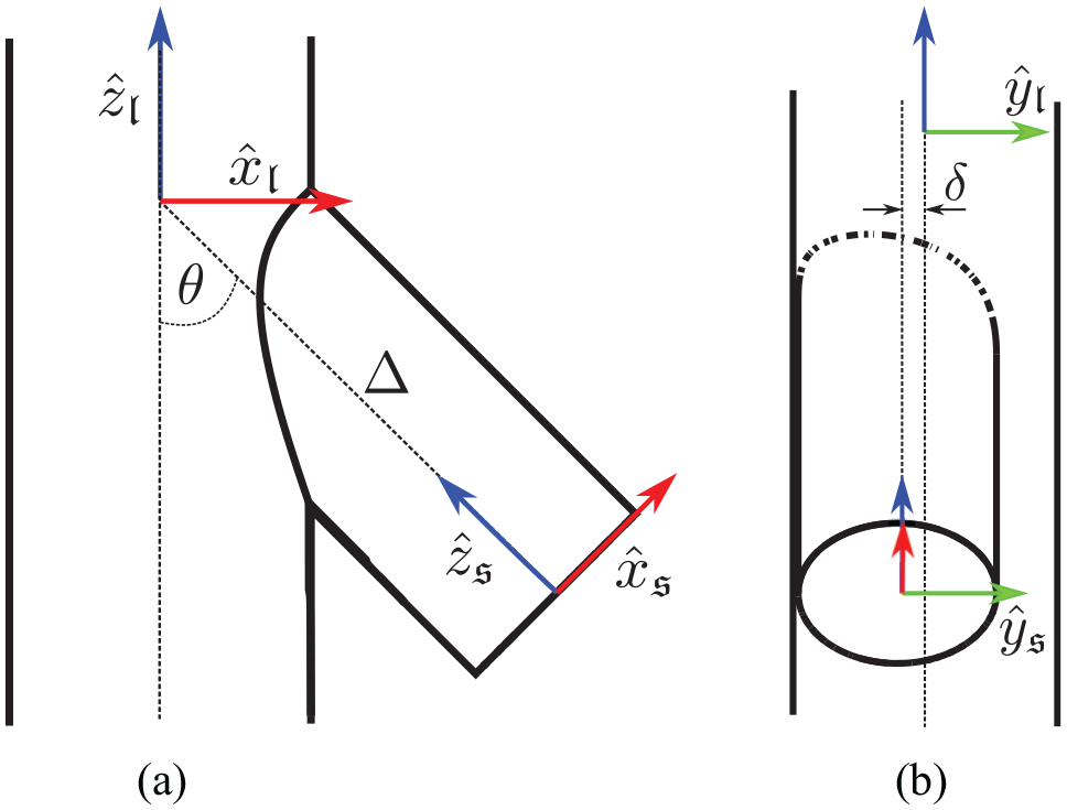
Illustration of the relative pose of the tubes in two different cross sections. (a) illustrates the pitch angle $\theta$ and the protrusion $\mathrm{\Delta }$ in the ${\hat{x}}_{\mathfrak{l}}-{\hat{z}}_{\mathfrak{l}}$ -plane, while (b) illustrates the offset $\delta$ in the ${\hat{y}}_{\mathfrak{l}}-{\hat{z}}_{\mathfrak{l}}$ -plane. Note that in the illustration, the offset is negative.

Figure 2.

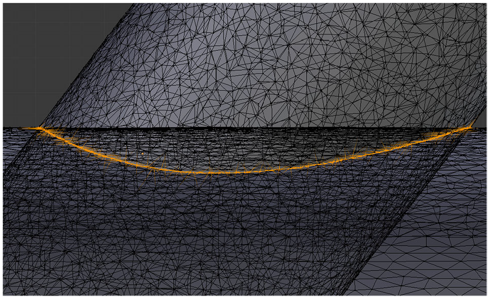
Illustration of the result of an intersection algorithm working on two tubular mesh components.

Figure 3.

Illustration of a cross section at point p in the ${\hat{n}}^{\mathfrak{s}}-{\hat{n}}^{\mathfrak{l}}$ -plane. Shown are the outside, outwards normal vectors, ${\hat{n}}^{\mathfrak{l}}$ and ${\hat{n}}^{\mathfrak{s}}$ ; the groove opening angle, ${\alpha }^c$ ; the cutting direction, ${\hat{d}}^c$ ; the welding angle, ${\alpha }^w$ , and direction, ${\hat{d}}^w$ ; the stub z-direction, ${\hat{z}}^{\mathfrak{s}}$ ; the stub-inwards and -outwards leg tangents in the cross section, ${\hat{t}}^{\mathfrak{l},\mathrm{in}}$ and ${\hat{t}}^{\mathfrak{l},\mathrm{out}}$ respectively; and the positive traversing path tangent $\hat{t}$ . Note that the inner and outer surfaces are illustrated as line segments in the graphics, but in general they are elliptical segments.

Prototype implementation and results

This section goes through elements of practical concern for the use and experimentation with the prototype software based on the mathematical formulations in section ‘Principle of solution’, and for processing real data with the prototype software. These elements regard generating synthetic models for experimentation; techniques to be applied if the real data are not externally corresponded to model references; and indication of the validity of the prototype software by illustrations over real, scanned meshes as well as stress testing with synthetic meshes.

The prototype software system is based on the 3D modelling platform Blender and the Python programming platform. Both are free software and have a couple of decades of development behind them so we consider them highly available and highly matured.

Generating synthetic mesh models

This section addresses the important topic of generating experiment data for the solution sketched in the previous section. The problem is the generation of realistic meshes to represent the tube surface models, as if they originated from a point cloud acquisition system. The main purpose of working with synthetic meshes is the ability to stress test by controlling the quality of the meshes, and the general speedup of experimenting with generated data without involving a laboratory set-up in the development loop.

The most realistic method would be to use a VR capturing process, which would even capture the artefacts incorporated by the manual operation. This is detailed by Danhof et al. ¹⁵ This is a comprehensive system to set-up, and it is not expected that the level of detail and trueness to reality is necessary. Besides, the system, such as it is presented, produces point clouds, but we expect the capturing system to produce mesh surfaces.

An easier option is to use Blender for modelling a cylinder mesh of the appropriate dimensions, deforming it according to the expected large scale deviations expected from the tubes. The Remesh tool in Blender is then used for uniform sub-sampling of the mesh to a specified resolution. This process is based on building an Octree to a specified depth. ¹⁶ Adding noise to the resulting vertices with the Randomize tool should generate sufficiently realistic data for our purpose. The resolution and level of noise should naturally be set at levels expected from the capturing system. To obtain a desired resolution for a given object, we must first calculate the corresponding Octree depth. If the longest length of the object is denoted by $L$ and the desired geometric resolution in terms of the neighbour vertices distance is denoted by $r$ , then we may calculate the required Octree depth $d$ as $d=\lceil \underset{2}{\log }\left(\frac{L}{r}\right)\rceil$ .

Figure 4 illustrates an example of processing a virgin cylindrical surface segment into a mesh which resembles the structure we will expect from a capturing system. Figure 4(a) illustrates a virgin cylinder segment with a diameter of 2 units, a length of 2 units and a resolution of 128 perimeter nodes. Figure 4(b) illustrates an Octree sub-sampling of the virgin cylinder segment with a depth of 5. The resulting resolution will thus be $r\approx \frac{\sqrt{2^2+2^2}}{2^5}\approx 0.08$ in the worst case, where the longest length, $L$ , of the object is $\sqrt{2^2+2^2}$ . Notice that some discretization error and irregularity enter. Figure 4(c) illustrates the result when adding an amount of $0.01$ units of uniform noise to the vertex positions. For illustration purposes the resolution is much lower and the noise is much higher than what we require of the capturing equipment, when we interpret the units in the model as metres.

Figure 4.

Illustration of processing a mesh to one which resembles the outcome of a real capturing system. Resolution and noise are exaggerated. (a) Virgin. (b) Remeshed. (c) Randomized.

For experiments a perfect cylinder segment is obviously not very interesting. Deformations should be introduced in the virgin model in Figure 4(a) prior to remeshing and randomizing. These deformations should be representative of the tubes found in the industrial applications; notably ovality and peaking, but also longitudinal variations if relevant.

Scanned tubes and captured meshes

At a demonstration of the Creaform HandySCAN 3D at Kværner Verdal AS, tubes for a real stub welding case were scanned. The tubes that were available are from a real construction application. However, they are not the same size as the target constructions for which the prototype software was developed. For testing the application, this is of minor importance.

The scanned stub and leg tubes were of a nominal outer radius of ${r^o}_{\mathfrak{s}}=305\mathrm{mm}$ and ${r^o}_{\mathfrak{l}}=611\mathrm{mm}$ , respectively. It is noteworthy, but not important for testing and illustration purposes, that the stub tube was too narrow for inside scanning with. Thus only the outer surface of the stub tube was scanned, whereas the prototype software actually needs the scan of the inner surface. In the testing and ensuing illustrations we used the captured stub mesh, as if it was captured by an inside scan.

Scanning with the Creaform HandySCAN 3D requires covering the target surface with small reflecting markers. The reflecting markers can be seen on the outside surface of the tubes in Figures 5(a) and (b). The markers are placed irregularly with an inter-spacing of approximately $20\mathrm{cm}$ . Figures 5(a) and (b) illustrate scanning of the marked leg and stub tubes, respectively.

Figure 5.

Scanning meshes with the Creaform ‘HandySCAN 3D’ scanner. [Courtesy Tony Melkild, MLT Maskin og Laserteknikk AS]. (a) Scanning of leg tube. (b) Scanning of stub tube. (c) Captured mesh (stub).

A close-up of the captured mesh from the scanning of the stub tube is shown in Figure 5(c). It exhibits very little surface noise, and the mesh is highly regular over large domains, and having no topological deficiencies.

The same process is used for producing the captured leg mesh. The scanned leg tube is seen in Figure 5(a), where the welding seam of the tube is also clearly visible. The region of the leg tube chosen for scanning, and subsequently placement of the stub, was deliberately chosen to include the welding seam.

The meshes produced by the metrology software can be specified down to sub-millimetre resolution. This is much better resolution than necessary for the application of cutting and welding the tube joint. The mesh we obtained for the leg tube was chosen at a resolution of $10\mathrm{mm}$ and the resolution of the mesh for the stub tube was chosen at $5\mathrm{mm}$ . Both of these resolutions are expected to be much better than required from a total application perspective, where many other inaccuracies enter. Figure 5(c) shows the captured mesh of the stub tube.

Correspondence between models and captured meshes

As mentioned in the introduction of section ‘Principle of solution’, at some point the correspondence between the design model of the tube joint and the captured meshes of the tube surfaces must be made. Unless the capturing system is integrated with other metrological systems at the shop-floor, this correspondence has to be made by analysis of the meshes and be based on observable markers of known location in the actual geometries. A simple procedure for establishing the correspondence based on such markers is explained in this section.

Analysing the mesh for a cylinder surface with a RANSAC method will give us the best matching axis line, and hence the line on which the origo of the tube reference lies, ${\mathrm{o}}^{\mathfrak{l}}$ or ${\mathrm{o}}^{\mathfrak{s}}$ , as well as the direction of the z-axes, ${\hat{z}}^{\mathfrak{l}}$ or ${\hat{z}}^{\mathfrak{s}}$ . We will also know the best matching cylinder surface model, since the analysis will give us the best matching radius of the tube.

At least three physical markers should be identifiable and set up in a non-symmetrical configuration. The positions that the markers indicate should be known in tube reference, that is, in $\mathcal{L}$ for the leg tube and in $\mathcal{S}$ for the stub tube. There is a slight difference between the cases for leg and stub tubes. The leg tube already has a working reference defined by punch marks on the tube around the joint curve area. These punch marks are observable via the on-site metrology system, and are obvious candidate locations for placing physical markers. The stub tube does not have any physical reference, which is essentially introduced by the cutting process; thought in practice the weld seam of the welded tube is always used in the toe of the saddle-cut. Hence with respect to the stub reference, we only need to relate the captured mesh to the machine reference. In essence this latter may be achieved by either controlling the tool to make an observably large cut into the tube end, at a position with known machine reference, which is trivial, since the tool is controlled in machine reference. It is worth noting that once the saddle-cut in the stub has been made, the fit-up process on the leg tube will arrange for the correct posing of the stub. That is, it is not necessary to further establish an identifiable reference on the cut stub, though it may later be desired if it optimizes the fit-up process.

Results with scanned and synthetic meshes

This section illustrates results obtained with scanned and synthetic meshes. Generation of synthetic meshes was discussed in section ‘Generating synthetic mesh models’. Mesh capturing with the Creaform HandySCAN 3D was discussed in section ‘Scanned tubes and captured meshes’.

Meshes for the scanned tubes, as presented in section ‘Scanned tubes and captured meshes’, were generated without any particular reference. To be able to process these meshes with the prototype software, for generating the resulting cutting path, the meshes need to be represented with an adequate reference.

While section ‘Correspondence between models and captured meshes’ speculates about how such correct correspondence between captured meshes and tube models may be systematically established, we have not implemented such a system yet. For generating results, manual fitting in Blender was used, whereby positioning and orienting tube references for the pertinent meshes obtained good enough accuracy for processing the joint intersection. Experimentation and initial validation of the prototype software is highly tolerant to the accuracy of the tube references, so the requirements to this manual placement of references were not too hard.

Figure 6 illustrates the result for captured meshes from the scanned tubes. Figure 6(a) illustrates the two meshes of the tubes posed in the specified relative pose. Note that the weld seam on the leg tube is visible, and that the stub tube is posed such that it strides the weld seam.

Figure 6.

Illustration of the result based on the captured meshes. (a) Leg and stub meshes in relative pose. (b) Cutting and welding path. (c) Model of the final stub.

Figure 6(b) shows the resulting path from the prototype implementation. Shown in the illustration are points for the intersection path, and each path point is annotated with the following interesting directions: path tangent, root weld approach direction, cutting approach direction, leg outward normal vector and stub-outward normal vector; see Figure 3 for details on these directions. A sort of validation is obtained when the annotated intersection path shown in Figure 6(b) is visually inspected in space, overlaid on the posed tubes shown in Figure 6(a). Errors in path positions or directions are very easily observed. This, however, is very hard to capture in static illustrations, since 3D orbiting and panning is required for such inspection to be complete.

Effects of the weld seam feature of the leg tube are visible in the illustration in Figure 6(b). These effects are hard to see from the intersection path points, but they are amplified and clearly observable in the direction vectors.

The finished stub-end which would result from the cutting process, based on the calculated cutting tool curve and known tube wall thickness, is shown in Figure 6(c). When this stub-end is overlaid on the leg tube surface from Figure 6(a) and a good match in both contact and groove opening is observed, it serves as a further visual validation that the calculation of the cutting path has been successful.

A series of tests have been conducted on synthetic mesh data. For all well-formed mesh pairs with a single closed intersection curve, the prototype implementation has proven successful.

Figure 7, following the same structure of illustrations as Figure 6, illustrates one case of meshes and the results of processing. Figure 7(a) illustrates the two meshes of the tubes posed in the specified relative pose. The example meshes shown are generated with a geometric resolution in the order of $0.1\mathrm{m}$ and the mesh point locations have been added a Gaussian noise in the order of $0.01\mathrm{m}$ . For testing and illustration purposes, strong deformations have also been added. The leg tube has bumps and an indentation while the stub tube has strong peaking. Figures 7(b) and (c) show the resulting direction-annotated path and stub-end, respectively.

Figure 7.

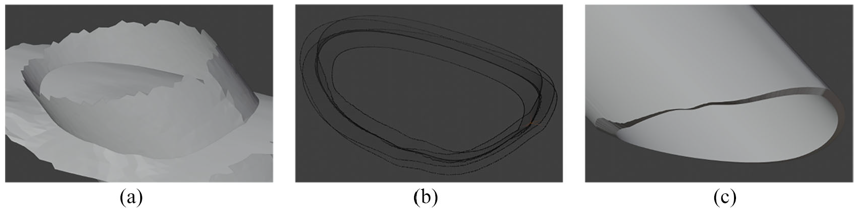
Illustration of a result based on heavily deformed, synthetic meshes. (a) Leg and stub meshes in relative pose. (b) Cutting and welding path. (c) Model of the final stub.

Conclusion and discussion

Many executions of the software have been performed on synthetic meshes generated with a broad variety of deformations, noise levels and geometric resolutions. As long as these deformations and noise levels stay within limits that leave the topology of the meshes well-formed and their relative pose maintains a single, closed intersection curve, the software have always produced correct results. By well-formed, we mean that the resulting meshes are not self-intersecting and that the resulting intersection curve can be parameterized by azimuth angle around the stub axis line; that is, the mesh intersection curve has exactly one solution for any azimuth angle.

In addition to the successful validation with synthetic meshes, one set of captured meshes from scanned tubes from a real application have been processed successfully.

Validation of the presented software up to this point has been based entirely on visual inspection of the processing results in 3D. The validity of the mesh intersection algorithm itself is taken for granted, as it is a third party tool. However, if the mesh intersection algorithm was invalid, it would have revealed itself in the visual inspection of the results. A final validation of the calculations of the presented software will be performed by measuring a cut stub tube and its root alignment on the leg patch it was cut to match.

So far no efforts have been invested in analysing pathological cases. We take the stance that it is the responsibility of the measurement system, or some intermediary mesh processing software system, to provide well-formed meshes that cover the specified intersection. Under this stance the presented system may be considered complete. Support for the realism in such a stance was obtained from the processing of the captured meshes.

Though the presented method and software may be considered complete for simple, outside weld joints, there are some known improvements and extensions that are desirable.

For convenience, the azimuth angle around the stub tube axis line was chosen as the parameter for the intersection curve. This in itself is natural and not an immediate problem. However, the sampling we use in the current version of the software is homogeneous in the azimuth. If the stub tube radius is close to the leg tube radius or if the stub offset is large, there will be sections of the intersection curve, where the path tangent deviates strongly from the maximum curvature tangent of the stub tube. The result is that the geometric resolution of the interpolated final path is strongly heterogeneous. This may not be a problem for the geometric accuracy or for the cutting machine, but if it is, a calculated, heterogeneous parameterization in the azimuth may be used for establishing geometric homogeneity of the interpolated intersection path. This improvement should address the calculation of ${\mathrm{\Phi }}^l$ in equation (2), where the target is a homogeneous azimuth resolution $\delta \varphi$ . A given, desired geometric path resolution, $r_p$ , should be the input to analysing the geometry and generating the corresponding azimuth interpolation base ${\mathrm{\Phi }}^l$ .

The initial specification for the prototype software was to correctly address outside welding joints; that is, joints that are only welded from the outside of the stub and leg tubes. These types of weld joints are the predominant ones in volume. However, a non-negligible amount of joints require mixed-side weld joints. These are joints with low pitch angle, see $\theta$ in Figure 1. When $\theta$ is low, the stub tube itself will become an access hindrance for welding around the heel of the joint. Such joints have an outside weld groove at the toe and an inside groove at the heel. Some specified region of the stub sides are dedicated for switching over between inside and outside grooves. In this region there is thus both an inside and an outside welding groove. This will require some further analysis and merging of the intersection paths arising from both the outside and inside surfaces of the stub tube with the outside surface of the leg tube.

In addition to these known improvements, it must be considered that the presented method is only implemented in a prototype software system. Interfaces with operators and other shop-floor IT systems, as well as deployment, must be taken into account further down the road.