
Abstract
In order to facilitate system design and performance analysis, a virtual prototype for metro train electropneumatic brakes is proposed. A virtual braking environment that consists of a three-car train model and six electropneumatic brakes model is elaborated. The virtual braking environment can be used to research the relation between braking response and electropneumatic brake’s parameters and to simulate axle loading transfer. By comparing the simulation results with bench test data, the electropneumatic brake model is proven to be quite accurate. Based on the proposed virtual prototype, a test train brake is designed, and a couple of field tests are carried out. The average deceleration of electropneumatic compound service brake at the initial speed of 45 km/h is 0.83 m/s2, the braking distance is 94 m, and that of pure air service brake at the speed of 43 km/h is 0.64 m/s2, the braking distance is 111 m. The field test results satisfy the test train requirements, which further proves the effectiveness of the proposed virtual prototype.
Introduction
Electropneumatic brakes are widely used on metro trains and high-speed trains because of its advantages over pneumatic brakes,1,2 and its performance directly affects the operation safety and quality of trains.3 Generally, to obtain the required braking performance (e.g. pressure response time, braking distance), engineers modify the parameters (e.g. cross-sectional areas of orifices, volumes of braking cylinder chambers) of a newly designed brake, which will require a large number of experimental tests. With the rapid development of metro train, the existing test platforms are not applicable to various electropneumatic brakes. It is related to different types of valves, cylinders, gas tubes, and other components. The workload is very large, and it also increases the experimental cost and time. As a result, mathematical and simulation models are adopted by researchers to analyze and simulate the functions of the braking system. Pugi et al.4–6 divided the braking system into basic elements, complex components, and vehicle subassembly, and the system model was established using MATLAB/Simulink. Moreover, the distribution valve and train tube models of the freight trains braking system were established using AMESim. W Wei et al.7–9 used the numerical calculation method to propose the braking system model of the freight trains and analyze its braking characteristics and longitudinal dynamics. Piechowiak10,11 presented detailed models for pneumatic brake of a freight train using a lumped parameter method. The papers mentioned above are limited to modeling the conventional pneumatic braking systems, which are seldom used now. As for the virtual modeling of electropneumatic braking systems, J-Y Zuo et al.12 and Q Lu and Yang.13 established the simulation model of subway train braking system through AMESim software. H-P Li et al.14 used AMESim to establish a braking system model for high-speed trains. The above works explored the feasibility of using AMESim software to study the modeling of electropneumatic braking systems, but few studies have been performed on the subject of modeling electropneumatic brakes in the MATLAB environment. In one of our previous studies,1 the model of an electropneumatic brake was built using MATLAB/Simulink and validated by comparison with experimental results. However, the final braking performance of an electropneumatic brake is affected by not only its structure parameters,15 but also other subsystems on the train, for example, vehicle dynamics,16–18 wheel–rail adhesion,19,20 and electric braking. Few studies have considered the effects of other subsystems during modeling the electropneumatic brakes.
In this paper, the virtual prototype method is applied to facilitate the development of metro train electropneumatic brakes. A virtual braking environment which consists of a three-car train model and six electropneumatic brakes model is elaborated. The virtual braking environment will help engineers to get a better understanding of the influences that other subsystems (e.g. vehicle dynamics and electric braking) will have on the performance of the electropneumatic brake. Therefore, parameters of a newly designed electropneumatic brake can be tested and optimized even before train braking tests.
This article is organized as follows. The “Virtual prototype” section gives details of a three-car train model and an electropneumatic brake model. The “Virtual prototype simulation verification” section gives some simulation results to verify the proposed virtual prototype. The “Field test verification” section introduces the test train brake and gives a couple of field test results to further verify the proposed virtual prototype. Finally, the research is summarized and conclusions are presented.
Virtual prototype
The virtual braking environment consists of a three-car train model and six electropneumatic brakes model (each one for each bogie). Figure 1 shows the topology of the virtual braking environment. During simulation, the electropneumatic brake will acquire the axle speeds and electric braking forces of each car from the train model and accordingly produce enough braking cylinder pressure to slow down or stop the train. The six electropneumatic brakes intercommunicate with each other so as to distribute braking forces on each car, and this intercommunication functionality is normally achieved through controller area network (CAN) bus on actual metro trains.

Topology of the virtual braking environment.
Train model
The train model consists of three cars. In order to reduce the number of state variables of the model and the amount of simulation operations, this article takes into account vehicle dynamics of 3 degrees of freedom (vertical, longitudinal, and nodding). They are closely related to train braking process, and less relevant degrees of freedom (rolling, yawing, and lateral) are neglected during modeling. Figure 2 shows the simplified model diagram of a car. In Figure 2, Lc is half of the distance between the two bogie centers of a car; Hc is the height of the centroid of a car body; Hcp is the height of a coupler; Hbci is the height of the acting point of the force between a car body and its bogie, i = 1 for front bogie and i = 2 for rear bogie; Hb is the height of the centroid of a bogie frame; lb is half of the distance between the two axles of a bogie; Rw is the rolling radius of a wheelset; Rbr is the equivalent braking radius of pneumatic braking force, and Rebr is the equivalent braking radius of electric braking force.

Model diagram of a car.
Moreover, modular modeling method is adopted, and the car is decomposed into four kinds of smaller components, that is, car bodies, bogie frames, wheelsets, and spring–dampers (primary suspensions, secondary suspensions, and the couplers). Each kind of component is modeled individually and then assembled to form a vehicle model using MATLAB/Simulink, and then the car models are assembled to build a three-car train model. The detailed modeling process is given as follows:
Car body
Figure 3(a) shows the force diagram of a car body. Based on D’Alembert’s principle,21 the equilibrium condition of forces in different directions can be described in the following.
Vertical
(a) Force diagram of a car body and (b) a car body Simulink block diagram.
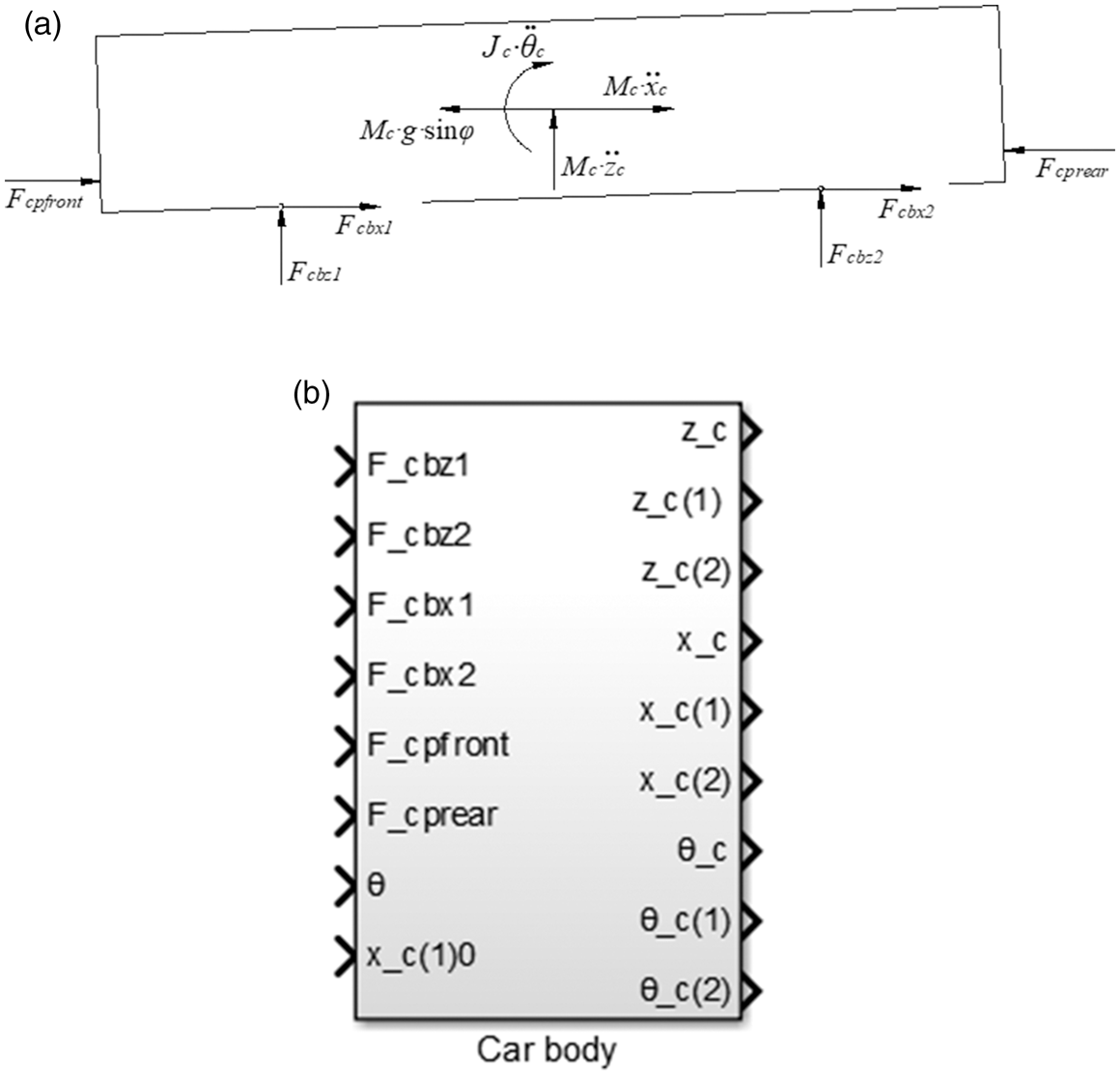

where Longitudinal

where Nodding

where
Based on equations (1)–(3), the simulation model of a car body can be built using MATLAB/Simulink (Figure 3(b)).
2. Bogie frame
Figure 4(a) shows the force diagram of a bogie frame. The equilibrium condition of forces in different directions can be described in the following.
Vertical
(a) Force diagram of a bogie frame and (b) a bogie frame Simulink block diagram.


where Longitudinal

where Fwxi is the longitudinal force between a bogie frame and its wheelset, i = 1 for front and i = 2 for rear wheelset.
Nodding

where
Using equations (4)–(6), the model of a bogie frame can be built using MATLAB/Simulink (Figure 4(b)).
3. Wheelset
Figure 5(a) shows the force diagram of a wheelset. In order to take into account wheel skidding during braking, a wheelset is described in two different cases, that is, the skidding case and the non-skidding case. A critical force Fcr is used to tell apart the working condition of a wheelset, and it can be calculated using the following equation
(a) Force diagram of a wheelset and (b) a wheelset Simulink block diagram.

In the non-skidding case (Fcr ≤ μrailFwN), the model of a wheelset is described by four equations


Then the wheelset model can be built using MATLAB/Simulink (Figure 5(b)) based on the equations above.
4. Spring–damper
Spring–dampers (Figure 6(a)) can be used to model the primary suspensions, the secondary suspensions, and the couplers of the metro train.
(a) Force diagram of a spring–damper and (b) a spring–damper Simulink block diagram.
The force of the spring–damper can be calculated as

Then the spring–damper model can be built using MATLAB/Simulink (Figure 6(b)) based on equation (16).
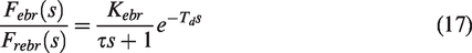
5. Electric braking force
The response of the electric braking force Febr in Figure 5 generated by a traction motor is simulated by using the first-order filter with time delay
Electropneumatic brake model
In this section, based on a more detailed model in the previous article,1 a structure-simplified model (Figure 7) of the electropneumatic brake is built in consideration of the following aspects:
The most important parameters which are related to the transient response performance of an electropneumatic brake are valve orifice diameters and chamber volumes, so the simplified structure mainly consists of two on/off solenoid valves and two chambers. From a mathematical and pressure control point of view, control valves in an actual brake (usually consist of on/off solenoid valves and piloted pneumatic valves) can be described as two on/off solenoid valves. Instead of being mounted near the braking cylinders, the pressure sensors are usually mounted at the output ports of a brake. Thus, an output chamber needs to be modeled individually. The short tubes connecting the output ports of the brake and the braking cylinders are simplified into an orifice because short tubes act like orifices. Simplified structure of the electropneumatic brake.

Pressure dynamics in the two chambers of the simplified brake structure in Figure 7 can be given as

The heat transfer process during air charging and discharging phases can be described as a polytropic process, which lies between isentropic and isothermal processes.22 Thus, air temperatures in the two chambers during air charging and discharging phase can be described as

Using the perfect gas equation, air temperatures in the chambers during a pressure holding phase can be described as

Mass flow rates

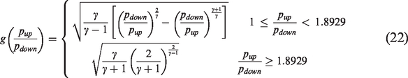
Using equations (18)–(22), the electropneumatic brake model can be built using MATLAB/Simulink.
Virtual prototype simulation verification
In this section, the braking response performance of the proposed virtual prototype is validated first, and then the axle loading transfer phenomenon is simulated based on the virtual prototype.
Braking response
The semi-physical simulation method is used to verify the virtual prototype. As shown in Figure 8, train brake hard-in-loop (HIL) test bench which is composed of data acquisition and signal conversion circuit and braking system hardware is elaborated. Driver controller produces brake command; the three-car train model runs in industrial computer and provides the axle speeds and electric braking forces for electropneumatic brakes. Braking system hardware mainly includes 3 brake supply air cylinders (100 L for each one), 6 electropneumatic brakes, and 12 analog braking cylinders (2 L for each one). In the test, the electropneumatic brake is controlled by a pulse width modulation (PWM)24–26 signal, whose period is 1.6 s with 0.4 s as an air charging phase and the other 1.2 s as a pressure holding phase. Figure 9 shows the performance of the proposed electropneumatic brake model and an actual brake.
Train brake HIL test bench.
For one thing, as shown in Figure 9(b), there is a sharp pressure jump in the output chamber at the beginning of brake application. This phenomenon is because the pressure sensors of an electropneumatic brake onboard a train are mounted at the output chambers of the brake instead of braking cylinder chambers. It takes a short period of time before the pressure signal in the output chamber reaches the braking cylinder, and pressurized air accumulates in the output chamber and this causes a sharp pressure jump. As we can see from the simulation results in Figure 9(a), this pressure jump phenomenon is closely predicted by the simulation model. For another thing, as shown in Figure 9(a) and (b), the pressure in the output chamber and braking cylinder slowly falls during the holding phase. This phenomenon is caused by the thermal exchange between the air and chamber walls. The temperature of air in the chambers is first higher than that of the chamber walls during the charging period and then it drops during the holding period.
Electropneumatic brake model performance: (a) simulation and (b) bench test.
As for the pressure oscillations in the holding phases in Figure 9(b), this phenomenon is caused by pressure waves traveling back and forth between the output chamber of the brake and the braking cylinder chamber during the holding phase. The damping of these oscillations is provided by the resistance forces in the pipes. But this feature is not focused on the proposed electropneumatic brake model (as shown in Figure 9(a)) by simplifying the pipes into orifices in this article. Thus, the proposed electropneumatic brake model simulation results can predict the performance of an actual brake. Without modifying an actual brake, one can tune the parameters (orifice diameters, chamber volumes, etc.) of the proposed electropneumatic brake model to study the relation between the response of a brake and its parameters.
Axle loading transfer
During the train’s braking process, the loading on some axles will get heavier than that in non-braking conditions, and others will be lighter, that is, the axle loading transfer happens. The loading seriously affects the use of adhesive weight. Moreover, the braking forces on different axles should be distributed accordingly so as to make full use of the available wheel–rail adhesion and avoid unnecessary wheel skidding at high braking levels.
In order to study the axle loading transfer phenomenon, a simulation test is conducted. The deceleration in this simulation test is 1 m/s2 with an initial train speed of 80 km/h. Figure 10 shows the axle loading of the four axles of the first car of the three-car train model during braking under the loading condition of AW0 (without passengers). As we can see, the loading on axle 2 is the biggest, and axle 3 is the smallest. The loading difference between axle 2 and axle 3 is approximately 8%. Therefore, using the proposed virtual prototype, engineers can study the axle loading transfer phenomenon at different braking decelerations and car weights.
Axle loading transfer of a car.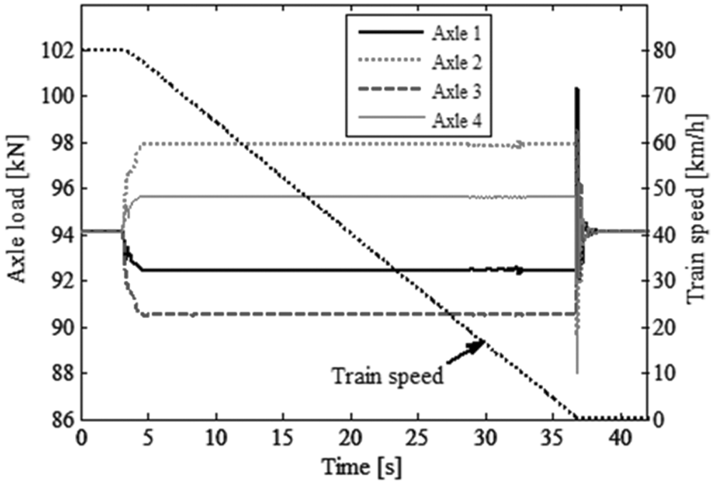
Field test verification
Test train brake
Based on the above-proposed virtual prototype, an actual brake is designed and applied to a test train. Metro train braking system mainly consists of air supply devices, brake electronic control unit (BECU), brake control unit (BCU), unit brake devices, and axle speed sensors. Figure 11 shows the test train and local diagrams of the components of the braking system. Air supply device supplies compressed air to the brake. BECU and BCU, as the core components in braking system, calculate, generate, and transfer braking force to unit brake devices. Unit brake device is the braking actuator to slow down or stop the train. Axle speed sensor detects axle speed and provides it to BECU for wheel anti-skid protection.
Test train.
Field test
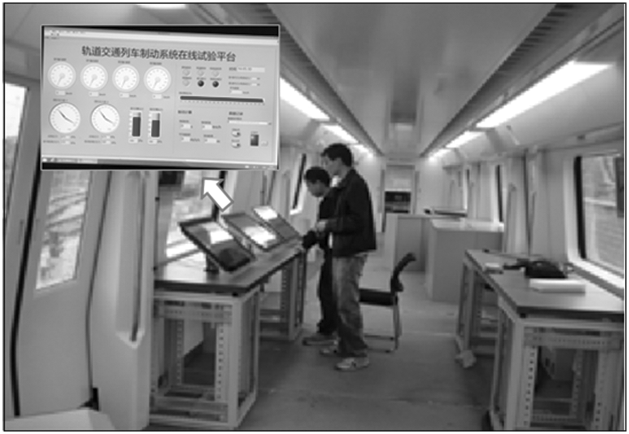
A couple of field tests (Figure 12) of the prototype train are carried out to further verify the proposed virtual prototype. The field tests consist of electropneumatic compound service brake test and pure air service brake test. The test data are collected and recorded by the tablet PC in Figure 12. Some of the data are analyzed and shown in the following.
Electropneumatic compound service brake test In order to verify the electric air matching ability of the brake, the electropneumatic compound service brake test is performed, and the electropneumatic compound service brake command is applied at the initial braking speed of 20, 30, and 45 km/h, respectively. Figure 13 shows the results of the trailer car at the initial speed of 45 km/h. It can be seen from Figure 13, trailer car brake cylinder pressure reaches 160 kPa at first and then increases to 320 kPa in the low-speed region. This is because there is an electric braking force produced by the traction motor, which undertakes part of the braking power for trailer car in high-speed region. The initial braking speed is 45 km/h, braking distance is 94 m, and the average deceleration is 0.83 m/s2. Pure air service brake test Similarly, the pure air service brake command is applied at the speed of 20, 30, and 45 km/h, respectively. Figure 14 shows the results of the trailer car at the initial speed of 45 km/h. It can be seen from Figure 14, trailer car brake cylinder pressure reaches 300 kPa, and there is no electric braking force. The initial braking speed is 43 km/h, braking distance is 111 m, and the average deceleration is 0.64 m/s2. According to the above field test results, it can be concluded that the prototype train brake based on the virtual prototype meets the test train requirements, which further verify the virtual prototype. Test site. The electropneumatic compound service brake results at the braking initial speed of 45 km/h. The pure air service brake results at the braking initial speed of 45 km/h.


Conclusion
In this article, a virtual prototype for metro train electropneumatic brake development is proposed. A virtual braking environment, which consists of a three-car train model and six electropneumatic brakes, is developed. The train model is proposed by assembling smaller component models including car bodies, bogie frames, wheelsets, and spring–dampers. Electropneumatic brake is modeled based on a simplified brake structure which mainly consists of two on/off solenoid valves and two chambers. A couple of simulation tests and field tests are carried out to justify the proposed virtual prototype. The research conclusions are as follows.
In the simulation tests, braking response simulation results can reproduce the performance of an actual brake. Axle loading transfer can be studied using the proposed virtual prototype at different braking decelerations and car weights. The electric air matching ability is verified in the electropneumatic compound service brake test. The field test results of braking distance and the average deceleration meet the test train requirements, which further verify the virtual prototype. Engineers can use the virtual prototype to tune and optimize the parameters of a newly designed electropneumatic brake before train braking tests. Moreover, engineers can get a better understanding of the influences that other subsystems (e.g. vehicle dynamics and electric braking) will have on the performance of the electropneumatic brake. The present models do not include the adhesion curves and the wheel slide protection (WSP) system. The next step is to research the relation between wheel–rail adhesion coefficient and slip rate based on brake test bench.
The method proposed in this article can also be applied to other rail transit braking system by modifying the virtual prototype.
Footnotes
Handling Editor: James Baldwin
Acknowledgements
The authors thank the brake control research group members in Brake Technology Research Center, Institute of Rail Transit, Tongji University, for many good suggestions and discussions.
Declaration of conflicting interests
The author(s) declared no potential conflicts of interest with respect to the research, authorship, and/or publication of this article.
Funding
The author(s) disclosed receipt of the following financial support for the research, authorship, and/or publication of this article: The authors also appreciate the support of the National Key Technology R&D Program in the 13th Five-year Plan of China (grant no. 2018YFB1201603-13).