Sage Journals: Discover world-class research

Abstract

A computational fluid dynamics (CFD) trimming method based on wind tunnel and flight test data is proposed. Aerodynamic coefficients obtained for a helicopter rotor using this method were compared with both experimental data from a test report and CFD results based on the control parameters that were reported in the same document. The method applies small disturbances to the collective pitch angle, the lateral cyclic pitch angle and the longitudinal cyclic pitch angle of the helicopter’s main rotor during forward flight to analyze the effects of each disturbance on the thrust coefficient, the pitching moment coefficient and the rolling moment coefficient of the rotor. Then, by solving a system of linear equations, the collective pitch angle, the lateral cyclic pitch angle and the longitudinal cyclic pitch angle of the main rotor in the CFD trim state are obtained. The AH-1G rotor is used in this paper. NASA has conducted a comprehensive flight test program on this model and has published detailed test reports. Using this method, the pitch moment and the roll moment can be corrected to almost zero and the calculated thrust coefficient is more consistent with the test data when compared with results from direct CFD simulations.

Keywords

Helicopter rotor trimming overset grid collective pitch cyclic pitch computational fluid dynamics

Introduction

As the most important part of a helicopter, the main rotor provides thrust, lift and the control force for the aircraft. The rotor’s aerodynamic performance is related directly to the dynamic characteristics of the entire helicopter. An extremely complex unsteady flow dynamic environment is formed within the flow field of a helicopter during forward flight. This environment includes the interactions of strong vortices with each other and with the rotor blades, the formation of a complex spiral wake behind the rotor, a transition between laminar flow and turbulence, wide variations in the Mach and Reynolds numbers on the blade, the local shock generated by an advancing blade and the airflow separation generated by a retreating blade.^1,2 These aerodynamic problems mean that research into the aerodynamic performance of helicopter rotors presents considerable challenges.

At present, experimental methods and computational fluid dynamics (CFD) methods are generally used to study the aerodynamic performance of helicopter rotors. Experimental methods provide a direct and reliable means for rotor aerodynamic research. When classical problems such as airframe drag reduction are considered, experimental methods using wind tunnels or water tunnels are sometimes more effective than CFD.^3,4 However, rotor flight experiments are very expensive and time-consuming and field visualization methods (e.g. particle image velocimetry) often have insufficient spatial resolution to enable detailed observation of the rotor flow field characteristics. In recent years, the rapid development of CFD methods and the increasing availability of low-cost computational power have allowed highly accurate aerodynamic simulations to be performed with short turnaround times. CFD methods have become an increasingly important means of research into a helicopter’s aerodynamic performance and can provide numerical solutions to the Navier–Stokes (N-S) governing equations for the entire flow region.⁵ Many new advances have been made in this field recently. Shi et al.⁶ developed a coupled fluid-structure method using a combination of a viscous wake model (VWM), CFD and comprehensive structural dynamics (CSD) modules for rotor unsteady airload prediction. Zhao et al.⁷ established a robust unsteady rotor solver Chinese Laboratory of Rotorcraft Navier–Stokes (CLORNS) code to predict the complex unsteady aerodynamic characteristics of the rotor flow field. Comparison of the numerical results simulated using their CLORNS code with test data illustrated that the proposed code could simulate the aerodynamic loads and the aerodynamic noise characteristics of helicopter rotors accurately.

Many advanced CFD technologies have been applied to CFD simulations of helicopter rotors.^8,9 Because it presents unique advantages, the overset grid method¹⁰ has attracted considerable attention in CFD simulations of helicopter rotors. This method is applicable to helicopter hover, forward flight, vertical flight and near-ground flight simulations and is the most widely used method in the helicopter aerodynamic simulation field. The method is thus also adopted in this paper and will be explained in detail in the following sections. Sliding grid technology is also often applied to the hovering conditions of the rotor. Steijl and Barakos¹¹ explained the principle of the sliding grid in detail and verified the accuracy of this method using several examples. The deformed mesh technique has also been widely used in rotorcraft CFD/CSD coupling-based simulation research. Among the available mesh deformation methods, one of the most popular is the spring analogy method. Bottasso et al.¹² improved this method to solve the defect that allowed mesh deformities to be formed easily and made the method suitable for handling of relatively large elastic deformation motions. Adaptive grid methods have been used widely to capture complex rotor wakes accurately. In some implementations, a Cartesian background grid is used to ease mesh refinement. The Helios project^{13, 14} in the United States has applied adaptive grid technology successfully to the capture of rotor vortex wakes and remarkable results have been achieved. Jameson and Mavriplis¹⁵ first introduced the multi-grid method into the central difference scheme, which accelerated the convergence of the solutions effectively. Later, Li et al.¹⁶ further developed a coarse mesh generation algorithm for unstructured multi-grids and demonstrated its good effect in accelerating the convergence. Nishikawa and Diskin¹⁷ applied the multi-grid method to the structured overset grid of a rotor and proved that the quality of the coarse grid could be better assured when using the structured multi-grid method, thus improving the accuracy of the calculations.

A variety of advanced methods are available for CFD simulations of rotors. However, regardless of the method that is adopted, the trimming of the rotor must be considered for CFD simulations of rotors during forward flight. Yang et al.¹⁸ used the traditional CFD trimming method to perform the trimming and flow field simulations of UH-60A and AH-1G helicopter rotors in the forward flight state. Embacher et al.¹⁹ also used the traditional CFD trimming method and selected the EC145 helicopter to verify their CFD model, which included the elastic motion of the rotor blades; they discussed the accuracy, convergence and stability of their method in detail. Although their trimming work produced reasonable results, the traditional CFD trimming method requires multiple iterations and thus involves a huge workload, which leads to low operational efficiency. Therefore, it is necessary to develop a new high-efficiency CFD trimming method.

To verify the accuracy of the calculations, the numerical results calculated using the CFD method must be compared with test data such as that obtained from wind tunnel or flight tests. Therefore, the working conditions used for the CFD method must be as similar as possible to the corresponding test conditions, including the rotor rotational velocity, the advance ratio, the rotor thrust coefficient, the rotor shaft angle, the collective pitch angle, the lateral cyclic pitch angle and the longitudinal cyclic pitch angle. Fortunately, several rotor test reports that contain detailed parameters or configurations for use in further study are always publicly available to researchers. The detailed parameters of the AH-1G rotor under various flight conditions that are used in this paper were disclosed by NASA.

In forward flight cases, the rotor has an asymmetrical aerodynamic load that leads to undesired moments with respect to the rotor hub. Therefore, rotor trimming becomes necessary to provide better agreement between the CFD results and the real test data. Specifically, the main rotor must satisfy the trimming conditions for the given force and moment, i.e. the rotor thrust is equal to the target thrust ( $C_{T} = C_{T}^{desired}$ ), and the pitching moment and the rolling moment are both zero ( $C_{M_{z}} = C_{M_{z}}^{desired} = 0, C_{M_{x}} = C_{M_{x}}^{desired} = 0$ ). However, the rotor control parameters obtained from flight tests during forward flight often contain small errors and it is difficult to ensure that the boundary conditions for the CFD simulation and those of the test environment are completely consistent. Therefore, if a CFD simulation is carried out directly using the control parameters measured in the flight test, the flow field calculation results are often not trimmed completely. Therefore, to improve the accuracy of CFD simulation results, it is necessary to use a CFD trimming method to trim the rotor based on the measured trimming control parameters ( $C_{T}, C_{M_{z}} and C_{M_{x}}$ ).

Methodology

Traditional trimming method

In general, there are three main control parameters that affect the trimming of the main rotor: the collective pitch $θ_{0}$ , the lateral cyclic pitch $θ_{1 c}$ and the longitudinal cyclic pitch $θ_{1 s}$ . To simplify the trimming process, the motion of the blade is generally assumed to be rigid and the flapping and lead-lag motions of the blade are thus ignored. The periodic blade pitch motion can be described as a function of the blade azimuth using the following equation, where $θ$ refers to the total pitch angle:^20,21.

θ = θ_{0} - θ_{1 c} \cos ψ - θ_{1 s} \sin ψ

(1)

The rotor’s aerodynamic response is a highly coupled function of the control parameters and the aerodynamic environment. The thrust produced by the rotor is mainly affected by the collective pitch but is also affected by both the lateral cyclic pitch and the longitudinal cyclic pitch. Similarly, the rotor’s roll and pitch moments are directly related to the cyclic pitch, but also cause thrust variations. These parameters are defined in the local coordinate system of the rotor disk as follows:

T = T (θ_{0}, θ_{1 c}, θ_{1 s})

(2)

M_{z} = M_{z} (θ_{0}, θ_{1 c}, θ_{1 s})

(3)

M_{x} = M_{x} (θ_{0}, θ_{1 c}, θ_{1 s})

(4)

where T is the thrust, $M_{z}$ is the pitch moment and $M_{x}$ is the roll moment.

The thrust coefficient, the pitching moment coefficient and the rolling moment coefficient of the rotor during the trimming process are given as follows:

C_{T} = \frac{T}{ρ π R^{2} {(Ω R)}^{2}}

(5)

C_{M_{z}} = \frac{M_{z}}{ρ π R^{3} {(Ω R)}^{2}}

(6)

C_{M_{x}} = \frac{M_{x}}{ρ π R^{3} {(Ω R)}^{2}}

(7)

where $ρ$ is the air density, R is the rotor radius, and Ω is the rotation velocity.

Figure 1 shows the definition of the rotor azimuth angle. The rotor drag is defined as the rotor force component in the freestream direction. The rotor thrust is the corresponding component in the direction normal to the rotor disc.

Figure 1.

Definition of the azimuth angle.¹

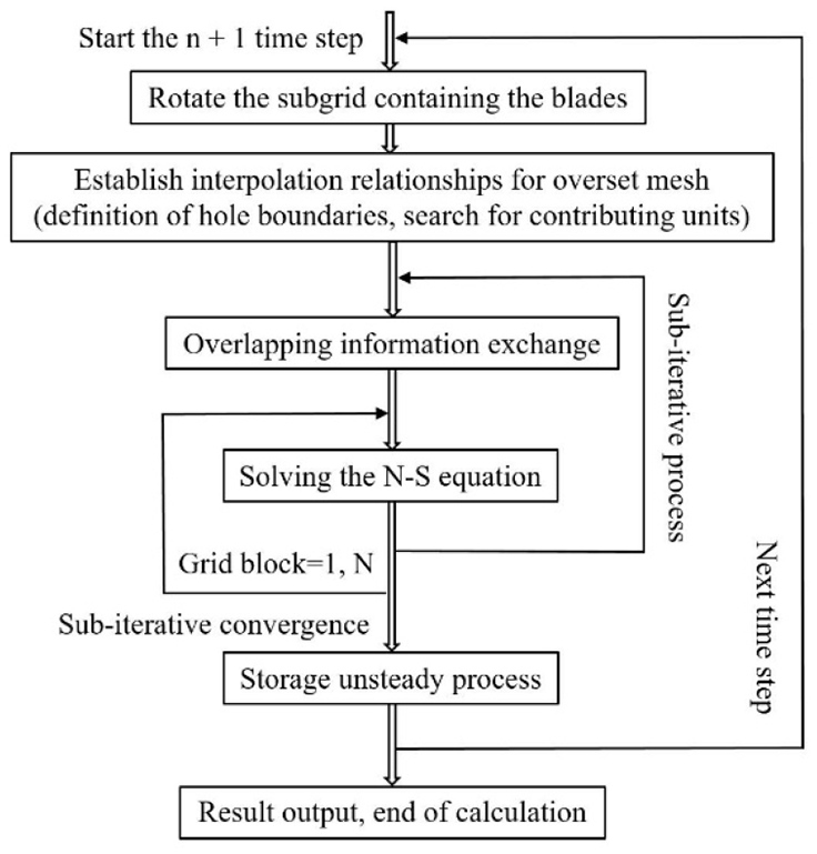
Figure 2 shows the flow chart for the traditional CFD trimming method,¹⁸ for which the steps can be described as follows.

Figure 2.

Flow diagram of traditional CFD trimming process.

First, the initial control parameters $(θ_{0}^{0}, θ_{1 c}^{0}, θ_{1 s}^{0})$ are given and the CFD method is used to calculate the thrust coefficient, the pitch moment coefficient and the roll moment coefficient of the rotor in its initial state.

Second, $θ_{0}^{0}, θ_{1 c}^{0}, θ_{1 s}^{0}$ are combined with the small additional perturbations $ε_{0}, ε_{1 c}, ε_{1 s}$ , respectively, to calculate the rotor thrust coefficient, the pitch moment coefficient and the roll moment coefficient in the corresponding state.

Third, the effect of each control parameter on the thrust coefficient, the pitch moment coefficient and the roll moment coefficient of the rotor can be obtained based on the previous control parameters and the calculation results.

Finally, the cumulative variation of the control parameters is obtained by performing n iterations of the above process and the corresponding thrust coefficient $C_{T}^{n}$ , pitch moment coefficient $C_{M_{z}}^{n}$ and roll moment coefficient $C_{M_{x}}^{n}$ can then be calculated. If $C_{T}^{n}$ , $C_{M_{z}}^{n}$ and $C_{M_{x}}^{n}$ meet the conditions that $| C_{M_{z}}^{n} | < δ_{1}$ , $| C_{M_{x}}^{n} | < δ_{2}$ and $| C_{T}^{desired} - C_{T}^{n} | < δ_{3}$ , then the trimmed state is considered to have been reached, and $θ_{0} = \sum_{i = 0}^{n} θ_{0}^{i}$ , $θ_{1 c} = \sum_{i = 0}^{n} θ_{1 c}^{i}$ , $θ_{1 s} = \sum_{i = 0}^{n} θ_{1 s}^{i}$ , $C_{T}^{desired} = C_{T}^{n}$ , $C_{M_{z}}^{desired} = C_{M_{z}}^{n}$ and $C_{M_{x}}^{desired} = C_{M_{x}}^{n}$ . Otherwise, the new control parameter set $θ_{0}^{n}, θ_{1 c}^{n}, θ_{1 s}^{n}$ must be taken as inputs and the process returns to the first step until the convergence condition is satisfied. Here, $δ_{1}, δ_{2}, δ_{3}$ are all positive numbers that are close to zero.

The trimming method based on the above process can be very tedious and may require multiple iterations, and the flow field simulation must also be carried out at each time step. In general, the flow field simulation of the main rotor is highly computationally intensive and requires a large amount of time per iteration. Therefore, a new trimming method is proposed in this paper that can greatly reduce the number of calculations and the time required for trimming and the results from this method are shown to be satisfactory.

New trimming method

Because the collective pitch, the lateral cyclic pitch and the longitudinal cyclic pitch calculated via trimming often differ slightly from the corresponding test data, it can be assumed that the effects of the collective pitch, the lateral cyclic pitch and the longitudinal cyclic pitch on the thrust, the pitch moment and the roll moment of a rotor are linear. Therefore, a linear equation system can be established and the collective pitch, the lateral cyclic pitch and the longitudinal cyclic pitch of the rotor in the CFD trim state can then be obtained by solving these equations. Figure 3 shows a flow chart for the new CFD trimming method proposed in this paper and the specific operational steps are described as follows.

Figure 3.

Flow chart for the new CFD trimming process.

First, given the control parameters, which are used to calculate the thrust coefficient, the pitching moment coefficient and the rolling moment coefficient of the rotor in its initial state, the test data are generally used as the initial control parameters when they exist, i.e.

θ_{0}^{0} = θ_{0}^{test}

(8)

θ_{1 c}^{0} = θ_{1 c}^{test}

(9)

θ_{1 s}^{0} = θ_{1 s}^{test}

(10)

Second, the small perturbation angles $ε_{0}, ε_{1 c}, ε_{1 s}$ are added to $θ_{0}^{0}, θ_{1 c}^{0}, θ_{1 s}^{0}$ , respectively, and used to calculate the thrust coefficients $C_{T}^{ε_{0}}, C_{T}^{ε_{1 c}}, C_{T}^{ε_{1 s}}$ , the pitching moment coefficients $C_{M_{z}}^{ε_{0}}, C_{M_{z}}^{ε_{1 c}}, C_{M_{z}}^{ε_{1 s}}$ and the rolling moment coefficients $C_{M_{x}}^{ε_{0}}, C_{M_{x}}^{ε_{1 c}}, C_{M_{x}}^{ε_{1 s}}$ of the rotor in the corresponding states.

Third, the effects of these small perturbation angles on the thrust coefficient, the pitch moment coefficient and the roll moment coefficient of the rotor can be obtained from the previous calculation results using the following.

Δ C_{T}^{ε_{0}} = C_{T}^{ε_{0}} - C_{T}^{0}

(11)

Δ C_{T}^{ε_{1 c}} = C_{T}^{ε_{1 c}} - C_{T}^{0}

(12)

Δ C_{T}^{ε_{1 s}} = C_{T}^{ε_{1 s}} - C_{T}^{0}

(13)

Δ C_{M_{z}}^{ε_{0}} = C_{M_{z}}^{ε_{0}} - C_{M_{z}}^{0}

(14)

Δ C_{M_{z}}^{ε_{1 c}} = C_{M_{z}}^{ε_{1 c}} - C_{M_{z}}^{0}

(15)

Δ C_{M_{z}}^{ε_{1 s}} = C_{M_{z}}^{ε_{1 s}} - C_{M_{z}}^{0}

(16)

Δ C_{M_{x}}^{ε_{0}} = C_{M_{x}}^{ε_{0}} - C_{M_{x}}^{0}

(17)

Δ C_{M_{x}}^{ε_{1 c}} = C_{M_{x}}^{ε_{1 c}} - C_{M_{x}}^{0}

(18)

Δ C_{M_{x}}^{ε_{1 c}} = C_{M_{x}}^{ε_{1 c}} - C_{M_{x}}^{0}

(19)

Fourth, equations are established to enable quantitative calculation of the effects of the collective pitch, the lateral cyclic pitch and the longitudinal cyclic pitch on the thrust coefficient, the pitch moment coefficient and the roll moment coefficient, respectively.

Δ C_{T}^{test} - C_{T}^{0} = X . Δ {C_{T}}^{ε_{0}} + Y . Δ {C_{T}}^{ε_{1 c}} + Z . Δ {C_{T}}^{ε_{1 s}}

(20)

C_{M_{z}}^{test} - C_{M_{z}}^{0} = X . Δ C_{M_{z}}^{ε_{0}} + Y . Δ C_{M_{z}}^{ε_{1 c}} + Z . Δ C_{M_{z}}^{ε_{1 s}}

(21)

C_{M_{x}}^{test} - C_{M_{x}}^{0} = X . Δ C_{M_{x}}^{ε_{0}} + Y . Δ C_{M_{x}}^{ε_{1 c}} + Z . Δ C_{M_{x}}^{ε_{1 s}}

(22)

Fifth, the collective pitch, the lateral cyclic pitch and the longitudinal cyclic pitch of the trimming state are obtained as follows.

θ_{0}^{trimming} = θ_{0}^{test} + X ε_{0}

(23)

θ_{1 c}^{trimming} = θ_{1 c}^{test} + Y ε_{1 c}

(24)

θ_{1 s}^{trimming} = θ_{1 s}^{test} + Z ε_{1 s}

(25)

Finally, the CFD simulation of the main rotor is performed using the collective pitch, the lateral cyclic pitch and the longitudinal cyclic pitch calculated using the new CFD trimming method to verify whether the calculated thrust coefficient is consistent with the value from the test data and whether the pitch moment coefficient and the roll moment coefficient are both close to zero.

Rotor model and CFD setup

In this paper, the aerodynamic characteristics of an AH-1G helicopter rotor during forward flight are selected for the numerical calculations. Flight testing was conducted on the AH-1G helicopter at the NASA Ames Research Center and the forward flight case selected here is test point No. 2157, which was reported by Cross and Watts.²² The rotor is composed of two blades with rectangular planes, an Operational Load Survey (OLS) airfoil and a linear twist of −10°. The flight conditions comprise an advance ratio of 0.19, a hover tip Mach number of 0.65, a flight Reynolds number of 9.73×10⁸, and a rotor thrust coefficient of 0.00464. These conditions correspond to a forward speed of 151.864 km/h at a rotor rotation rate of 315.9 rpm. It is then simple to calculate that the rotor rotation cycle is 0.19 s based on the data provided above.

The flight conditions selected for the validation case come from the flight tests documented by Cross and Watts²² and by Cross and Tu.²³ These tests were chosen because of their extensive load surveys, their acoustic measurements, and the detailed blade harmonics data provided. In addition, these flight conditions have been verified via a variety of other numerical methods,^9,18,20,24 which all provided results that show good correlation with the flight test data.

In this work, the flow simulations are based on the unsteady Reynolds-averaged N-S equations. The fluid is modeled as a compressible ideal gas. The Spalart–Allmaras (S-A) turbulence model²⁵ is used to estimate the eddy viscosity of the flow field. This model is based on use of a single transport equation for the eddy viscosity coefficient, with coefficients that were fitted using an extensive set of experimental data. The S-A model has been used widely in the aviation field, particularly in shock capture.

In the analysis in this paper, the rotor motion is modeled using the overset grid method,¹⁰ including the rotation of the main rotor and the periodic variation in the blade pitch angle.

This method allows us to divide the flow field into several subdomains and then generate grid blocks for each subdomain. The different grid blocks can overlap, nest or cover each other, thus reducing the difficulty of the grid generation process and compensating for the poor adaptability of the structural grid to the actual shape. The core technique of the approach involves the blocks “digging holes” in each other to establish the connections between the grid blocks. When applied to the flow problem of multi-body relative motion, these grid blocks have relative motion, and it is thus necessary to apply the overset grid technique at each time step to establish the connection relationships between these grid blocks and to transmit the boundary information from the interface required for the flow field calculations in each region. The overset grid technique consists of three steps: digging holes, searching for contribution units and interpolation.

Figure 4 shows an example in which an airfoil’s curvilinear grid lies within a background Cartesian grid. The airfoil grid captures features including the boundary layers, the tip vortices and shocks. The background grid surrounds the airfoil grid and carries the solution to the far field. This background grid was generated using some knowledge of the airfoil’s surface and the outer boundary locations. Consequently, some of the existing background grid points lie within the airfoil’s solid body regions and must therefore be removed from the solution. When these points are removed, hole regions remain within the interior of the larger background grid and this creates a set of boundary points known as the hole-fringe points. The airfoil grid interpolates the data to the background grid at the background’s hole-fringe points. Conversely, the background grid also interpolates data to the airfoil grid at the airfoil’s outer boundary points.²⁴

Figure 4.

Schematic of the overset grid system.

During the process of overset grid generation, to guarantee the quality of the solution interpolation at the boundaries, it is necessary to ensure that the boundaries have adequate overlap, nearly equal mesh sizes and low skewness. Simultaneously, high flow gradients should also be avoided at the boundaries.

In this paper, a structured grid is used to build the overset grid system, which is mainly composed of two grid types, where the first is an O-H type grid around the blade, which moves with the rotor. To simulate the viscosity effect effectively, the mesh was compacted at the leading edge, the trailing edge and the blade tip. The height of the first grid layer from the blade surface is $1.0 \times 10^{- 5} c$ , where $c$ is the chord length of the blade. The second grid type is the stationary background grid nested on the blade grid. The upper boundary of the background grid is 3R from the rotor disc plane, the lower boundary is 5R from the rotor disc plane and the circumferential boundary is 5R from the blade tip, where R is the blade radius. To capture the vortex at the blade tip accurately and also reduce the numerical dissipation, the relevant areas are encrypted in the background grid. Grid systems with total numbers of grids of approximately 12 million, 10 million, 8 million, and 6 million were simulated. It was found from these simulations that when the number of grids reached approximately 8 million, further increases in the number of grids would not then affect the results. When the number of grids is approximately 6 million, the simulation results obtained do not capture the vortex satisfactorily. Therefore, the total number of grid cells was eventually limited to approximately 8 million. The moving overset grid is shown in Figure 5.

Figure 5.

Schematic diagram of the AH-1G helicopter rotor moving overset grid system.

The overset grid method simplifies the arbitrary blade motions greatly, which is important when attempting to achieve trimmed flight conditions and predict airloads accurately. Additionally, overset grids allow the domain to be discretized more easily with simple well-defined grids that compute the rotor wake accurately.

The finite volume scheme is used to discretize the meshes for the rotor flow field. Various interpolation schemes have been developed based on the discrete method with inviscid flux at the interfaces of the grid elements. The central finite volume scheme is unsuitable for simulation of the unsteady characteristics of the rotor flow field because it has only second-order accuracy and artificial dissipation. Therefore, the Roe scheme,²⁶ which is an upwind scheme, has been used in this article. This scheme has a strong shock capture ability and calculates the numerical flux using an approximate Riemann solver.

Use of the Roe scheme’s approximate Riemann solver may lead to nonphysical solutions. Therefore, the eigenvalues in the Roe scheme are modified using the entropy correction method proposed by Harten and Hyman.²⁷

To provide the solution for the unsteady flow field of the rotor, the N-S equation is matched implicitly in time using the dual stepping method proposed by Jameson.²⁸

Figure 6 shows a flowchart for the dual time stepping method with overset grids. The blade overset regions move to new positions and interpolate with the background grid at the relevant intersections, thus rebuilding nested relationships with the background grid, and then enter the inner loop of the dual time stepping method. During each iteration, overlapping information is exchanged between the blade grid and the background grid and multiple grids are calculated block-by-block. When the sub-iteration process reaches convergence, the process enters the next physical time step. When the performance of the computer used in the laboratory was taken into account, the N-S equation was solved with a rotation angle of 3° and 20 sub-iterations per physical time step; if the rotation angle for each time step was smaller or the number of sub-iterations for each time step was higher, longer calculation times would be required when using the current laboratory computer. To shorten the calculation time required, the CFD simulation was only carried out for around three rotation cycles. The results became quasi-periodic after approximately 1.5 rotations.

Figure 6.

Flow diagram of the dual time stepping method for the overset grid.

For the unsteady N-S equation, the dual time stepping method performs a pseudo-time iteration for each physical time step, which is equivalent to solution of the steady-state problem. Therefore, accelerated convergence measures in the steady-state solution such as use of local time steps and implicit residual smoothing can be applied to this method. At present, the dual time stepping method is used widely in unsteady CFD simulations of rotors.

The far-field boundary adopted is a nonreflective boundary,²⁹ i.e. the disturbance wave will not be reflected back to the flow field. Reflectionless boundaries are defined using Riemann invariants³⁰ ( $R^{+}$ and $R^{-}$ ).

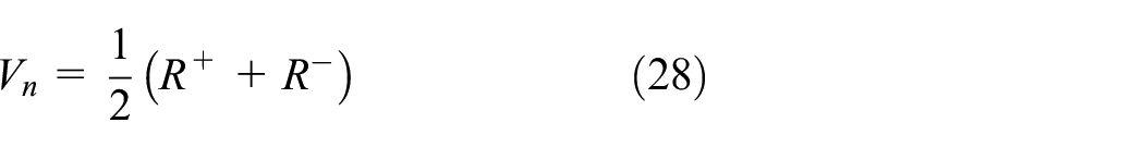
In this paper, the inlet and outlet boundaries of the computational domain are all in the subsonic state. For subsonic inflow and outflow, $R^{+}$ is computed by interpolation, while $R^{-}$ is computed based on the value of the incoming stream at infinity, i.e.

R^{+} = V_{ne} + \frac{2 c_{e}}{γ - 1}

(26)

R^{-} = V_{n \infty} - \frac{2 c_{\infty}}{γ - 1}

(27)

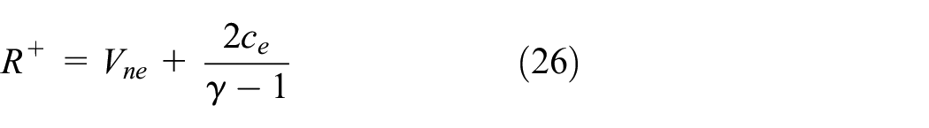
where n represents the normal direction and the subscripts $\infty$ and $e$ represent the incoming flow value and the infield value, respectively.

From equations (26) and (27), the normal velocity $V_{n}$ and the sonic velocity $c$ on the boundary can be derived as:

V_{n} = \frac{1}{2} (R^{+} + R^{-})

(28)

c = \frac{γ - 1}{4} (R^{+} - R^{-})

(29)

Let $V_{t}$ represent the tangential velocity and let s represent the entropy. For the subsonic inflow boundary ( $V_{r} < 0$ ):

V_{t} = V_{t \infty}

(30)

s = s_{\infty}

(31)

For the outflow boundary ( $V_{r} > 0$ ):

V_{t} = V_{te}

(32)

s = s_{e}

(33)

No penetration condition is required on the blade surface. When the N-S equation is used, the relative velocity of the airflow on the blade surface with respect to the blade motion velocity is zero, i.e.

\vec{V} - {\vec{V}}_{blade} = 0

(34)

where $\vec{V}$ and ${\vec{V}}_{blade}$ represent the air movement velocity and the blade surface velocity, respectively.

In addition, the blade surface must meet the thermal insulation conditions, i.e. the normal gradient of the temperature and pressure characteristic is zero.

\frac{\partial T}{\partial n} = 0

(35)

\frac{\partial p}{\partial n} = 0

(36)

For the rotor flow field during forward flight, the initial conditions are taken to be the values of the incoming flow at infinity:

(ρ, u, v, w, p) = (ρ_{\infty}, u_{\infty}, v_{\infty}, w_{\infty}, p_{\infty})

(37)

For the S-A turbulence model used in this paper, the initial conditions for the corresponding vortex turbulence motion viscosity coefficient $v$ are²⁵

\frac{3.0}{Re} < \tilde{v} < \frac{5.0}{Re}

(38)

Results and discussion

Table 1 shows the control parameters as measured during the flight test and calculated by CFD trimming under flight state conditions; slight differences can be seen between the two sets of parameters.

Table 1.

Control parameters of AH-1G rotor obtained from test data and CFD trimming.

Control parameters^a	$θ_{0}$	$θ_{1 c}$	$θ_{1 s}$
Test data	6.0°	1.7°	−5.5°
CFD trim results	6.28°	1.35°	−5.24°

θ ₀: collective pitch; θ_1c: lateral cyclic pitch; θ_1s: longitudinal cyclic pitch.

As physical time passes, some fluctuations will occur in the monitoring results from the CFD method that must be smoothed. The simple moving average (SMA) was used as the tool to solve this problem in this work. The older data are dropped when new data become available, thus causing the average to move along the timeline. This is achieved by averaging the number of data points n contained in the SMA. Using this method, the calculated results can be determined more easily and the resulting fluctuations can be suppressed.

SMA = \frac{x_{M} + x_{M - 1} + x_{M - 2} + \dots + x_{M - (n - 1)}}{n}

(39)

Figure 7 clearly shows that the thrust coefficient, the pitch moment coefficient and the roll moment coefficient calculated using the control parameters obtained via CFD trimming are more consistent with the results from the test report than the corresponding coefficients calculated using the control parameters from the test data. If the control parameters of the test data are set directly in the CFD simulation for further study, the main rotor may not be fully trimmed as a result.

Figure 7.

Comparisons of final coefficients. (a) $C_{M_{z}}$ vs. t; (b) $C_{M_{x}}$ vs. t; (c) $C_{T}$ vs. t.

Figure 8 shows the pressure coefficient distributions on the blade surface as calculated using the control parameters from CFD trimming and the control parameters from the test data and compares these distributions with the results from the test report. When compared with the pressure coefficient on the blade surface calculated using the control parameters from the test data, the pressure coefficient on the blade surface calculated using the control parameters from CFD trimming is observed to be in better agreement with the reported results from the test, particularly in terms of the shock wave capture on the leading edge of the blade’s upper surface.

Figure 8.

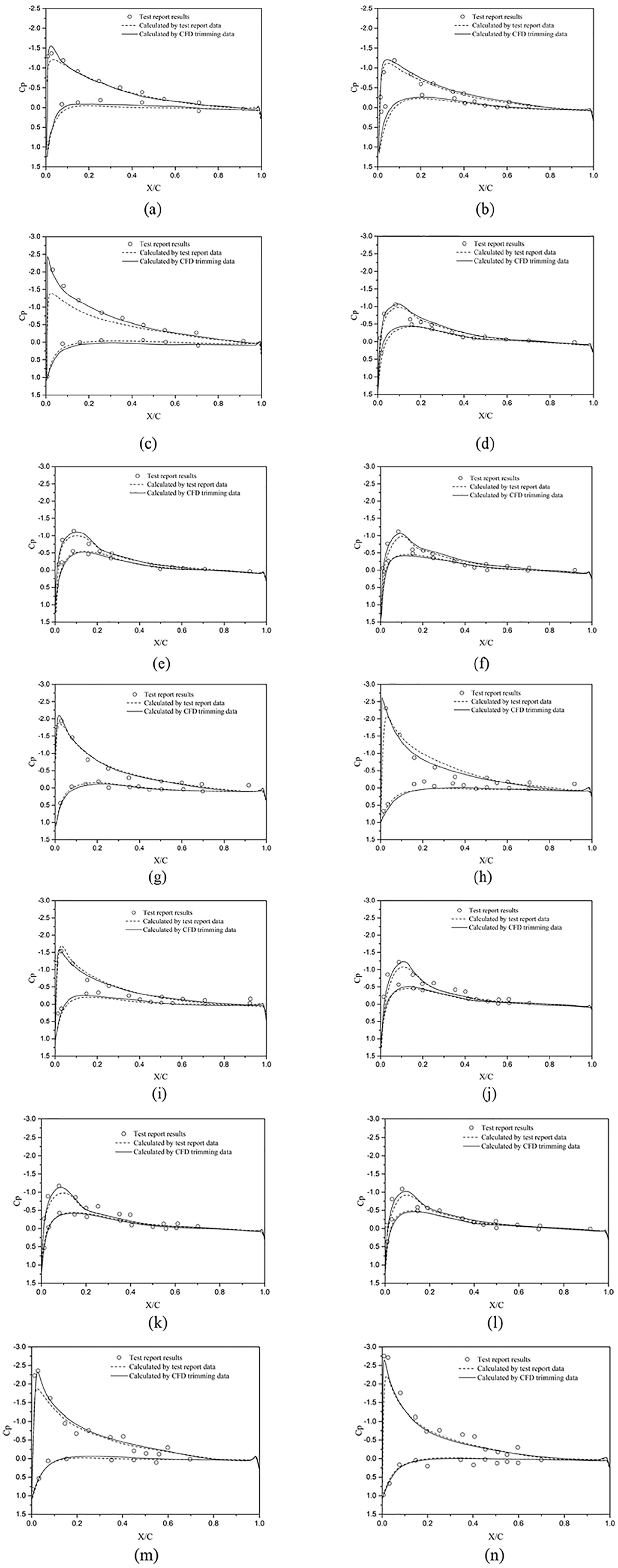
Pressure coefficient distributions at different azimuths and for different blade profiles (μ=0.19).

Figure 9 shows the normal force coefficients for the different sections and azimuth angles on the blade as calculated using the control parameters from CFD trimming and the control parameters from the test report and compares these coefficients with the results from the test report. As this figure shows, when the azimuth angle of the advancing blade is in the range from 70 to 90° or the azimuth angle of the retreating blade is in the vicinity of 270°, a relatively strong blade-vortex interaction phenomenon occurs that results in a dramatic change in the normal force coefficients, which then makes it difficult to calculate the aerodynamic force of the rotor during forward flight accurately. In addition, it is shown that when compared with the aerodynamic mutation calculated directly using the control parameters from the test report, the aerodynamic mutation obtained using CFD trimming is in better agreement with the results given in the test report, thus indicating that the control parameters obtained via CFD trimming are more accurate.

Figure 9.

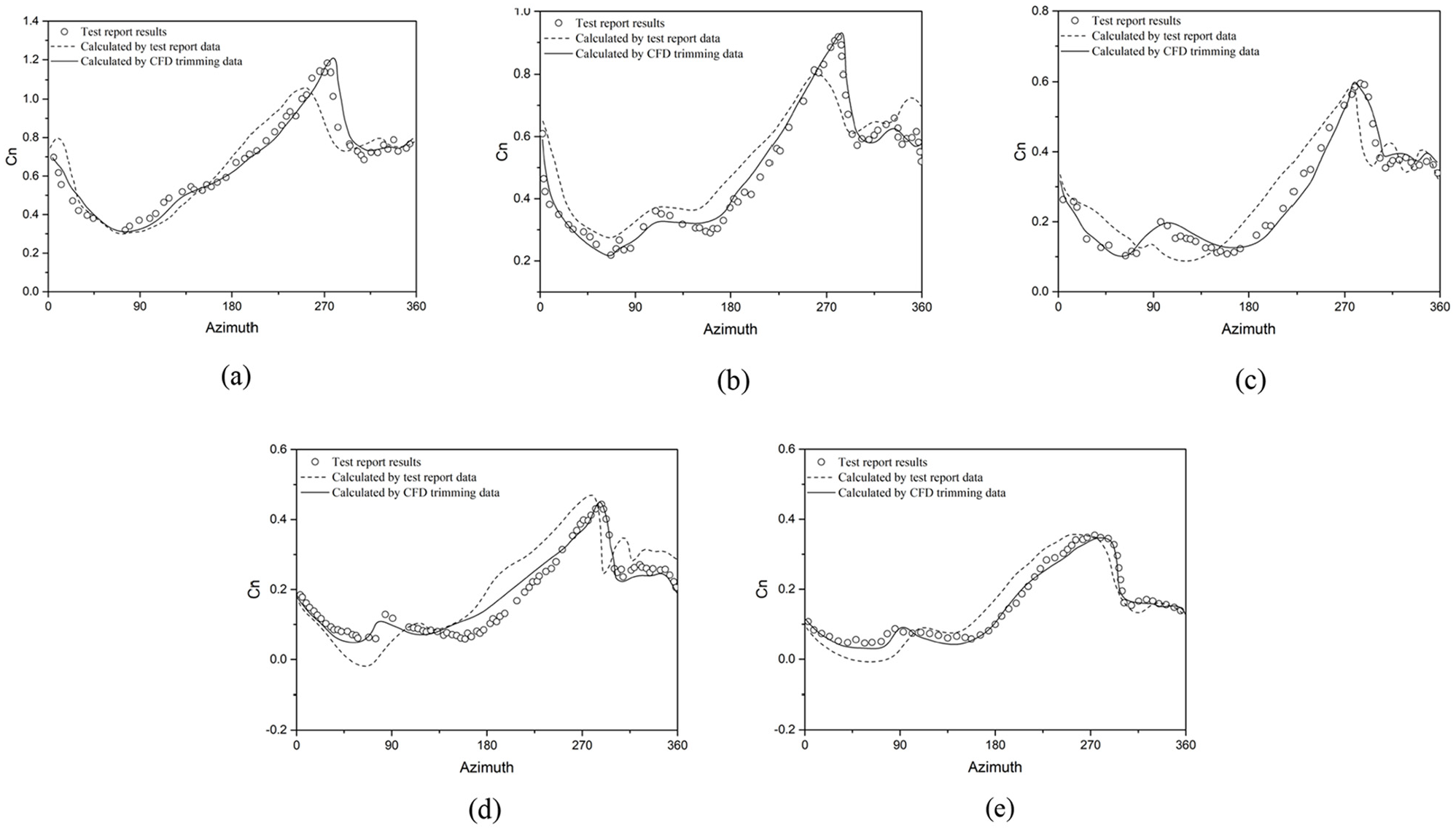
Normal force coefficients of an AH-1G rotor at different azimuth angles ( $μ = 0.19$ ).

Figures 7 to 9 demonstrate that the collective pitch angle, the lateral cyclic pitch angle and the longitudinal cyclic pitch angle calculated via the CFD trimming method proposed in this paper are better than the corresponding values calculated from the test data, which is helpful in improving the accuracy of simulation results of forward flight.

In the absence of control parameters being provided in a test report, the control parameters can now be estimated. When there is a major difference between the estimated value and the final trim value, the effects of the control parameters on the thrust, the pitch moment and the roll moment of the rotor may be nonlinear, and the trimming method proposed in this paper may then require two to three iterations to achieve a satisfactory trimming state. Table 2 shows the iterative process results when there is a large initial difference between the estimated control parameters and the final CFD trim values for the AH-1G rotor.

Table 2.

Iterative process with estimated control parameters.

Control parameters^a	$θ_{0}$	$θ_{1 c}$	$θ_{1 s}$
Estimated value	8°	3°	−3°
First iteration	6.55°	1.59°	−4.92°
Second iteration	6.34°	1.39°	−5.2°
Third iteration	6.29°	1.34°	−5.26°

θ ₀: collective pitch; θ_1c: lateral cyclic pitch; θ_1s: longitudinal cyclic pitch.

p < .10. *p < .05. **p < .01. ***p < .001.

After three iterations, the rotor basically reached the CFD trimming state and it was then found that the final trimming control parameters were very close to those obtained based on the test report, as presented in Table 1.

Therefore, in the absence of test data, the control parameters can be estimated using the proposed method and the new trimming method proposed in this paper can achieve a satisfactory trimming state after only two to three iterations. Although the proposed approach is more complicated than the trimming process performed with the test data, it is still much simpler than the traditional CFD trimming method.

Conclusions

In this paper, a new CFD trimming method is proposed for a helicopter rotor in forward flight and the rotor trimming process is introduced in detail. In the verification example for the proposed method, the detailed test parameters for an AH-1G rotor provided by NASA were adopted. The control parameters obtained by trimming and the control parameters used in the test report are both used to perform the simulations. The pitch moment coefficient, the roll moment coefficient, the thrust coefficient, the pressure coefficient and the normal force coefficient of the blade profile are calculated at different azimuth angles and are then compared with the relevant data in the test report, thus verifying the correctness and feasibility of the proposed trimming method.

This method avoids the disadvantages of the traditional CFD trimming method, which requires multiple iterations and performs multiple CFD simulations of the main rotor, thus greatly reducing the trimming workload and optimizing the trimming process. However, the proposed CFD trimming method is not perfect. The method ignores the flapping and lead-lag motions of the blades at present and assumes that the blades move rigidly. In future work, CFD/CSD coupling of the blades will be considered for the trimming method and the flapping and lead-lag motions of the blades must also be considered, although this will indeed be a difficult task. At the same time, use of an increased grid density in the area of interest and adoption of smaller time steps will be helpful in improving the accuracy of the CFD simulations.

Footnotes

Handling Editor: James Baldwin

Declaration of conflicting interests

The author(s) declared no potential conflicts of interest with respect to the research, authorship, and/or publication of this article.

Funding

The author(s) disclosed receipt of the following financial support for the research, authorship, and/or publication of this article: This research was financially supported by the National Key Research and Development Project of China (No. 2017YFD0701004).

ORCID iD

Chenglong Zhou

References

Leishman

. Principles of helicopter aerodynamics. New York: Cambridge University Press, 2006.

Conlisk

. Modern helicopter aerodynamics. Annu Rev Fluid Mech 1997; 29: 515–567.

Burley

Brooks

Rozier

, et al. Rotor wake vortex definition–evaluation of 3-C PIV results of the HART-II study. Int J Aeroacoust 2006; 5: 1–38.

Komerath

Smith

Tung

. A review of rotor wake physics and modeling. J Am Helicopter Soc 2011; 56: 22006-1–22006-19.

Badcock

Richards

Woodgate

. Elements of computational fluid dynamics on block structured grids using implicit solvers. Progr Aerosp Sci 2000; 36: 351–392.

Shi

, et al. A coupling VWM/CFD/CSD method for rotor airload prediction. Chin J Aeronaut 2017; 30: 204–215.

Zhao

Wang

, et al. Robust Navier-Stokes method for predicting unsteady flowfield and aerodynamic characteristics of helicopter rotor. Chin J Aeronaut 2018; 31: 214–224.

Brocklehurst

Barakos

. A review of helicopter rotor blade tip shapes. Progr Aerosp Sci 2013; 56: 35–74.

Tejero

Doerffer

Szule

, et al. Numerical simulation of the tip aerodynamics and acoustics test. J Therm Sci 2016; 25: 153–160.

10.

Benek

Bunimh

Steger

. 3-D chimera grid embedding technique. In: AIAA 7th computational physics conference, New York, NY, USA, 1985, paper no. CP854, pp. 322–331. New York: AIAA.

11.

Steijl

Barakos

. Sliding mesh algorithm for CFD analysis of helicopter rotor-fuselage aerodynamics. Int J Numer Meth Fl 2008; 58: 527–549.

12.

Bottasso

Detomi

Serra

. The ball-vertex method: A new simple spring analogy method for unstructured dynamic meshes. Comput Meth Appl Mech Eng 2005; 194: 4244–4246.

13.

Wissink

Potsdam

Sankaran

, et al. A coupled unstructured-adaptive Cartesian CFD approach for hover prediction. In: 66th American Helicopter Society international annual forum proceedings, Phoenix, AZ, USA, May 11–13 2010, vol. 2, pp. 1300–1317. Alexandria: American Helicopter Society.

14.

Lim

Wissink

Jayaraman

, et al. Application of adaptive mesh refinement technique in Helios to blade-vortex interaction loading and rotor wakes. In: 67th American Helicopter Society international annual forum proceedings, Virginia Beach, VA, USA, May 3–5 2011, vol. 1, pp. 228–250. Alexandria: American Helicopter Society.

15.

Jameson

Mavriplis

. Finite volume solution of the two-dimensional Euler equations on a regular triangular mesh. AIAA Journal 1986; 24: 611–618.

16.

Wang

Cao

, et al. An aspect ratio agglomeration multigrid for unstructured grids. Int J Numer Methods Fluids 2013; 72: 1034–1050.

17.

Nishikawa

Diskin

. Development and application of parallel agglomerated multigrid method for complex geometries. In: 20th AIAA computational fluid dynamics conference, Honolulu, HI, USA, June 27–30 2011, pp. 2514–2528. New York: AIAA.

18.

Yang

Sankar

Smith

, et al. Recent improvements to a hybrid method for rotors in forward flight. J Aircr 2002; 39: 804–812.

19.

Embacher

Keβler

Dietz

, et al. Coupled CFD-simulation of a helicopter in free-flight trim. In: 66th American Helicopter Society international annual forum proceedings, Phoenix, AZ, USA, May 11–13 2010, vol. 3, pp. 1976–1990. Alexandria: American Helicopter Society.

20.

Ramachandran

Schlechtriem

Caradonna

, et al. Free-wake computation of helicopter rotor flowfields in forward flight. In: AIAA 23rd fluid dynamics, plasma dynamics, and lasers conference, Orlando, FL, USA, July 6–9 1993. New York: AIAA.

21.

Johnson

. Helicopter theory. Princeton: Princeton University Press, 1980.

22.

Cross

Watts

. Tip aerodynamics and acoustics test: A report and data survey. Report for the National Aeronautics and Space Administration. Report no. NASA Ref. Pub. 1179, Dec 1988.

23.

Cross

. Tabulation of data from the tip aerodynamics and acoustics test. Report for the National Aeronautics and Space Administration. Report no. TM-102280, Nov 1990.

24.

Ahmad

Duque

. Helicopter rotor blade computation in unsteady flows using moving overset grids. J Aircr 1996; 33: 54–60.

25.

Spalart

Allmaras

. One-eq40 turbulence model for aerodynamic flows. Recherche Aerospatiale 1994; 1: 5–21.

26.

Roe

. Approximate Riemann solvers, parameter vectors, and difference schemes. J Comput Phys 1997; 135: 250–258.

27.

Harten

Hyman

. Self adjusting grid methods for one-dimensional hyperbolic conservation laws. J Comput Phys 1983; 50: 235–269.

28.

Jameson

. Time dependent calculations using multigrid, with applications to unsteady flows past airfoils and wings. In: 10th Computational fluid dynamics conference, Honolulu, HI, USA, June 24–26 1991. New York: AIAA.

29.

Hirsch

Verhoff

. Far field numerical boundary conditions for internal and cascade flow computations. In: 9th Computational fluid dynamics conference, Buffalo, NY, USA, June 13–15 1989. New York: AIAA.

30.

Jameson

Schmidt

Turkel

. Numerical solution of the Euler equations by finite volume methods using Runge Kutta time stepping schemes. In: 14th Fluid and plasma dynamics conference, Palo Alto, CA, USA, June 23–25 1981. New York: AIAA.

Computational fluid dynamics trimming of helicopter rotor in forward flight

Abstract

Keywords

Introduction

Methodology

Traditional trimming method

New trimming method

Rotor model and CFD setup

Results and discussion

Conclusions

Footnotes

Declaration of conflicting interests

Funding

ORCID iD

References