Applications of Legendre spectral collocation method for solving system of time delay differential equations

Abstract

The numerical techniques are regarded as the backbone of modern research. In literature, the exact solution of time delay differential models are hardly achievable or impossible. Therefore, numerical techniques are the only way to find their solution. In this article, a novel numerical technique known as Legendre spectral collocation method is used for the approximate solution of time delay differential system. Legendre spectral collocation method and their properties are applied to determined the general procedure for solving time delay differential system with detail error and convergence analysis. The method first convert the proposed system to a system of ordinary differential equations and then apply the Legendre polynomials to solve the resultant system efficiently. Finally, some numerical test problems are given to confirm the efficiency of the method and were compared with other available numerical schemes in the literature.

Introduction

Delay differential equations (DDEs) have been applied to model some real phenomena in a wide range of chemical, physical, engineering and biological systems and their networks. In mathematical Biology delay plays a crucial role is drug therapy for the disease of human immunodeficiency virus (HIV) infection.^1,2 These equations are called functional differential equations,^3,4 which is a special class of differential equations. DDEs were initially introduced In the eighteenth century, by Condorcet and Laplace. ⁵

In recent research, there are many other authors which studied the numerical approximate solution of DDEs. For more detail we refer the reader to Bellen and Zennaro, ⁶ and Feldstein and Neves. ⁷ Most of the DDEs solver are build up by using the adapted continuous numerical techniques for solving ordinary differential equation. To obtain the approximate solutions of DDEs on non-grid points, a local interpolation is needed. In such situation, stability of discrete method may be lost. The stable interpolant concept were introduced by Bellen and Zennaro, ⁸ for Runge–Kutta methods. In other words, a stable interpolant keep up the stability possessions of the proposed method itself. Hermite interpolation can be also used to solve a DDEs numerically. For the numerical solution of a DDEs the Oberle and Pesch, ⁹ are combined Hermite interpolation and Runge–Kutta methods, where they show that this combination has high order of accuracy and it is reliable.

Nevertheless, the most popular discrete methods are Runge–Kutta methods that use interpolation to obtain the numerical solution of a DDEs. Wherever, to produce results at specified points often the step size must be reduced, otherwise a Runge–Kutta formula becomes inefficient. Also Bogacki and Shampine, ¹⁰ have presented a structural way to handle this issue. When a high order method for solving a DDE is applied, the amount of computations for the interpolation process increases considerably. To overcome this difficulty, Zennaro ¹¹ presented a one-step collocation method. Also, for super convergence rate Wang and Wang, ¹² proposed the single-step and a multiple-domain Legendre-Gauss collocation integration processes for nonlinear DDEs. One of the most important advantages of their method is its accuracy and efficiency.

Another class of numerical methods that can be considered are Spline methods. ¹³ So far, all of the mentioned methods for solving a DDE have linear or quadratic order of convergence. To get exponential order of accuracy for a smooth problem, usually spectral methods are applied. For more details about these methods, see for example Gottlieb and Orszag. ¹⁴ The shifted Legendre polynomials have been employed by Ito et al., ¹⁵ to construct a spectral approximate solution for a DDE. More precisely, they considered Legendre-tau method to construct an approximate solution to a DDE with one constant delay. Also, for the approximate solution of pantograph type DDEs the numerical scheme are proposed by Sedaghat et al. ¹⁶ Similarly, Haar wavelet method applied by Aziz and Amin, ¹⁷ to obtain the numerical solution of DDEs. Ghasemi and Tavassoli Kajani ¹⁸ employed Chebyshev wavelets to obtain a numerical scheme for solving DDEs. They introduced operational matrix of delay and utilize it to reduce the solution of system of time-varying delay to the solution of algebraic equations. Similarly for the linear time delay systems, M Mousa-Abadian and SH Momeni-Masuleh ¹⁹ apply the Chebyshev-tau method.

Recently, S Yi et al., ²⁰ studied the solution of linear DDEs system by Laplace transformation method. M Pospíšil and F Jaroš, ²¹ studied the approximate solution of DDEs using the Laplace transformation. G Jin et al., ²² studied, the stability analysis method of the periodic DDEs with time-periodic and multiple delays. D Lehotzky et al., ²³ extended the stability and convergence analysis of spectral-element-method for the periodic time DDEs with distributed and multiple delays. Also SU Değer and Y Bolat, ²⁴ studied, the asymptotic stability of time delay system. According to the best of author knowledge, there are no such article in literature that addressed the solution of system of linear time DDEs by spectral collocation method. In this work, we use application of Legendre spectral method for the approximate solution to the system of linear time DDEs. Legendre spectral collocation method is also applied for the numerical solution of delay differential and stochastic DDEs. ²⁵ Also, for solving system of nonlinear Fredholm integral equations of second kind, stochastic Volterra integro differential equations and stochastic SIR (Susceptible Infected Recoverable) models are solved by Legendre spectral method.^26–28

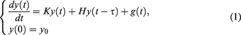
In this research work, we propose a new computational technique based on Legendre spectral collocation method (LSCM) for solution of system of time DDEs. Consider time delay system

$$\{\begin{array}{l}\frac{dy(t)}{dt}=Ky(t)+Hy(t-\tau )+g(t)\text{,}\hfill \\ y(0)=y_0\hfill \end{array}$$

(1)

In equation (1), $y_0$ is the initial condition, for all $t\in [0\text{,\hspace{0.17em}}{t}_i]$ , where $i\text{,\hspace{0.5em}}j=0\text{,}1\text{,}\dots \text{,}N$ .

 (a) $y(t)=[y_0(t)\text{,\hspace{0.17em}}{y}_1(t)\text{,}\dots \text{,}{y}_N(t{)]}^T$ with $y\in C([0\text{,}{t}_i]\text{,}{\mathrm{ℝ}}^{N+1})$ which are unknowns.

(b) $H\text{,\hspace{0.17em}}K$ , and $g$ are given functions having the following forms:

$g(t)=[g_0(t)\text{,\hspace{0.17em}}{g}_1(t)\text{,}\dots \text{,}{g}_N(t{)]}^T$ with $g\in C([0\text{,}{t}_i]\text{,}{\mathrm{ℝ}}^{N+1})$

$$H=\left(\begin{array}{cccc}{H}_{00}& \text{.}\text{.}& \text{.}\text{.}& H_{0N}\\ :& \text{.}& \hspace{0.17em}& :\\ :& \hspace{0.17em}& \text{.}& :\\ H_{N0}& \text{.}\text{.}& \text{.}\text{.}& H_{NN}\end{array}\right)$$

and

$$K=\left(\begin{array}{cccc}{K}_{00}& \text{.}\text{.}& \text{.}\text{.}& K_{0N}\\ :& \text{.}& \hspace{0.17em}& :\\ :& \hspace{0.17em}& \text{.}& :\\ K_{N0}& \text{.}\text{.}& \text{.}\text{.}& K_{NN}\end{array}\right)$$

with $H_{ij}\text{,}{K}_{ij}\in C([0\text{,}{t}_i]\text{,}\mathrm{ℝ})$ .

where $C(E\text{,}{\mathrm{ℝ}}^{N+1})$ the space of continuous and ${\mathrm{ℝ}}^{N+1}$ -valued functions on $E$ , and $E$ is topological space.

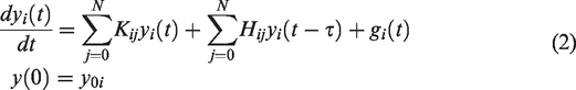
Observe that the system equation (1) has $i$ -equations takes the form

$$\begin{array}{l}\frac{d{y}_i(t)}{dt}={\displaystyle \sum _{j=0}^N}{K}_{ij}{y}_i(t)+{\displaystyle \sum _{j=0}^N}{H}_{ij}{y}_i(t-\tau )+g_i(t)\hfill \\ y(0)=y_{0i}\hfill \end{array}$$

(2)

where $y(0)=[y_{00}\text{,\hspace{0.17em}}{y}_{01}\text{,}\dots \text{,}{y}_{0N}{]}^T\text{.}$

For the LSCM, we expand the approximate solution using a finite Legendre series, associated with Legendre Gauss-Lobatto (LGL) nodes to evaluate the expansion coefficients. Such algorithm is easily implemented for the numerical solution especially time delay system. Moreover, the consistency and convergence of the LSCM are provided. For the validation, some numerical results are presented, which demonstrate the accuracy and efficiency of the Legendre spectral method.

This article is structured as follows. Description of the Legendre spectral method are given in the next section, which is followed by error and convergence analysis. Some test problems are given in the following section, and finally conclusion is given in the last section.

Legendre spectral method

This section describes some basic properties of the LSCM for solving numerically the system of time DDE equation (2). To consider the grid points ${\left\{t_k\right\}}_{k=0}^N$ , which is the set of $N+1$ LGL points in interval $[-1\text{,}1]$ , also we assume that the degree of real polynomials space ${\mathrm{\mathbb{P}}}_N$ is strictly less then $N$ .

First taking integral on both sides of equation (2) from $[0\text{,}{t}_i]$ gives the following form

$$y_i(t)=y_{0i}(t)+{\displaystyle \sum _{j=0}^N}{\displaystyle {\int }_0^{t_i}}{K}_{ij}(t\text{,}s)y_i(s)\text{d}s+{\displaystyle \sum _{j=0}^N}{\displaystyle {\int }_0^{t_i}}{H}_{ij}(t\text{,}s)y_i(s-\tau )\text{d}s+{\displaystyle {\int }_0^{t_i}}{g}_i(s)\text{d}s$$

(3)

Since we apply the Legendre polynomial which are orthogonal on $[-1\text{,}1]$ interval, to analyzed the interval of equation (3) on $[-1\text{,}1]$ interval, we take the following linear transformation given in following form $s=\frac{t_i}{2}(\theta +1)$ , then equation (3) becomes

$$\begin{array}{l}{y}_i(t)=y_{0i}(t)+\frac{t_i}{2}{\displaystyle \sum _{j=0}^N}\left[{\displaystyle {\int }_{-1}^1}\left(K_{ij}\left(t\text{,}\frac{t_i}{2}\left(\theta +1\right)\right)y_i\left(\frac{t_i}{2}\left(\theta +1\right)\right)\right)\text{d}\theta \right]\\ +\frac{t_i}{2}{\displaystyle \sum _{j=0}^N}\left[{\displaystyle {\int }_{-1}^1}\left(H_{ij}\left(t\text{,}\frac{t_i}{2}\left(\theta +1\right)\right)y_i\left(\frac{t_i}{2}\left(\theta +1\right)-\tau \right)\right)\text{d}\theta \right]+G_i(t_i)\end{array}$$

(4)

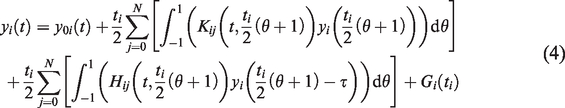
where $G_i(t_i)={\displaystyle {\int }_0^{t_i}}{g}_i(s)\text{d}s\text{.}$ For simplicity, let ${\eta }_{ik}=\frac{t_i}{2}(\theta +1)\text{,}$ where $k=0\text{,}1\text{,\hspace{0.17em}}\dots \text{\hspace{0.17em},}N$ . Now by using $(N+1)$ LGL points, the Gauss-quadrature concern with Legendre weight function, then the integral of equation (4) leads to semi-discretised spectral equation which takes the form

$$\begin{array}{l}{y}_i(t)=y_{0i}(t)+\frac{t_i}{2}{\displaystyle \sum _{j=0}^N}{\displaystyle \sum _{k=0}^N}\left(K_{ij}\left(t\text{,}{\eta }_{ik}\right)y_i\left({\eta }_{ik}\right){\omega }_k\right)\\ +\frac{t_i}{2}{\displaystyle \sum _{j=0}^N}{\displaystyle \sum _{k=0}^N}\left(H_{ij}\left(t\text{,}{\eta }_{ik}\right)y_i\left({\eta }_{ik}-\tau \right){\omega }_k\right)+G_i(t_i)\end{array}$$

(5)

where ${\omega }_k$ is the weight function given by

$${\omega }_m=\left\{\frac{2}{(1-x_m^2)[L_{N+1}^{\prime }(x_m{)]}^2}\right\}\text{,}0<m<N$$

where $L(x)$ represents the Lagrange interpolation polynomial. Suppose that $Y(t_m)\hspace{0.17em}\approx \hspace{0.17em}y(t_m)$ , and therefore, we are assume that Legendre spectral solution is given in the form

$$y(t)\hspace{0.17em}\approx \hspace{0.17em}Y(t):={\displaystyle \sum _{m=0}^N}y(t_m)P_m(t)$$

(6)

where in equation (6) $P_m(t)$ is Legendre interpolating polynomials associated with LGL points ${\left\{t_k\right\}}_{k=0}^N$ .

The Legendre polynomials of order $N$ are denoted by $P_N(t)$ . These polynomials are either even or odd, depends on even or odd orders of $N$ . The first few Legendre polynomials are given below. ²⁵ $P_0(t)=1$ , $P_1(t)=t$ , $P_2(t)=\frac{1}{2}(3t^2-1)$ , $P_3(t)=\frac{1}{2}(5t^3-3t)$ , $P_4=\frac{1}{8}(35t^4-30t^2+3)$ $P_5=\frac{1}{8}(63t^5-70t^3+15t)$ .

The generalized formula is given by:

$$P_n(t)=\frac{1}{2^n}{\displaystyle \sum _{k=0}^{\left[\frac{n}{2}\right]}}{(-1)}^k\left({\hspace{0.17em}}_k^n\right)\left({\hspace{0.17em}}_n^{2n-2k}\right)t^{n-2k}\text{,}(n=0\text{,}1\text{,}2\text{,}\dots \text{,}N)$$

(7)

$$\left[\frac{n}{2}\right]=\{\begin{array}{ll}\frac{n}{2}\text{,}\hfill & n\mathit{even}\text{,}\hfill \\ \frac{n-1}{2}\text{,}\hfill & n\mathit{odd}\text{.}\hfill \end{array}$$

Applying equation (6) to equation (5), the numerical scheme takes the form

$$\begin{array}{l}{Y}_i(t)\hspace{0.17em}\approx \hspace{0.17em}{y}_{0i}(t)+\frac{t_i}{2}{\displaystyle \sum _{m=0}^N}{Y}_m\left[{\displaystyle \sum _{j=0}^N}{\displaystyle \sum _{k=0}^N}\left(K_{ij}(t\text{,}{\eta }_{ik})y_i({\eta }_{ik}){\omega }_k\right)\right]\\ +\frac{t_i}{2}{\displaystyle \sum _{m=0}^N}{Y}_m\left[{\displaystyle \sum _{j=0}^N}{\displaystyle \sum _{k=0}^N}\left(H_{ij}(t\text{,}{\eta }_{ik})y_i({\eta }_{ik}-\tau ){\omega }_k\right)\right]+G_i(t_i)\end{array}$$

(8)

Now setting the following $Y:=[Y_0\text{,}{Y}_1\text{,}\dots \text{,}{Y}_N{]}^T$ and $F_N:=[y_{0i}(t)\text{,}{y}_{0i}(t)\text{,}\dots \text{,}{y}_{0i}(t{)]}^T+{[G_i(t_0)\text{,}{G}_i(t_0)\text{,}\dots \text{,}{G}_i(t_N)]}^T$ , therefore using this we get a more appropriate form of equation (8)

$$Y-({\mathrm{\varrho }}_1+{\mathrm{\varrho }}_2)Y=F_N$$

(9)

where ${\mathrm{\varrho }}_1\text{,}{\mathrm{\varrho }}_2\in R^{(N+1)\times (N+1)}$ and the entries of matrices are given below

$${\mathrm{\varrho }}_1(i\text{,\hspace{0.17em}}m)=\frac{t_i}{2}{\displaystyle \sum _{j=0}^N}{\displaystyle \sum _{k=0}^N}{K}_{ij}(t\text{,}{\eta }_{ik})y_i({\eta }_{ik}){\omega }_k$$

$${\mathrm{\varrho }}_2(i\text{,\hspace{0.17em}}m)=\frac{t_i}{2}{\displaystyle \sum _{j=0}^N}{\displaystyle \sum _{k=0}^N}{H}_{ij}(t\text{,}{\eta }_{ik})y_i({\eta }_{ik}-\tau ){\omega }_k$$

Convergence analysis

In this section, we perform the convergence analysis of the LSCM for the numerical solution to the system of time DDE given in equation (1). Once again for simplification, we defined following notations:

Assume $E=[0\text{,}{t}_i]$ , we equipped $C(E\text{,}{\mathrm{ℝ}}^{N+1})$ with sup-norm, $\mathrm{\parallel }y\mathrm{\parallel }={{\displaystyle \max }}_{t\in E}\mathrm{\parallel }y(t){\mathrm{\parallel }}_{\infty }$ whenever $y\in C(E\text{,}{\mathrm{ℝ}}^{N+1})$ . For $u=[u_0\text{,}{u}_1\text{,}\dots \text{.}\text{,}{u}_N{]}^T\in {\mathrm{ℝ}}^{N+1}\text{,}\mathrm{\parallel }u{\mathrm{\parallel }}_{\infty }={{\displaystyle \max }}_{i=0\text{,}1\text{,}\dots \text{,}N}|u_i|$ . However, for each continuous function $I:E^2\to {\mathbb{M}}_{N+1}(\mathrm{ℝ})$ , we have define $\mathrm{\parallel }I\mathrm{\parallel }={{\displaystyle \max }}_{(t\text{,}s)\in E^2}\mathrm{\parallel }I(t\text{,}s){\mathrm{\parallel }}_{\infty }$ .

Throughout, in $C(E^2\text{,}\mathrm{ℝ})$ we use the Schauder bases and Banach fixed-point (BFP) theorem.

Definition 1.

Consider if $f$ is a self-mapping in $E$ , where $E$ be a real Banach space, and let $r\in [0\text{,}1]$ for all $x_1\text{,}{x}_2\in E\text{,}\mathrm{\parallel }f(x_1)-f(x_2)\mathrm{\parallel }\le r\mathrm{\parallel }{x}_1-x_2\mathrm{\parallel }$ . ¹⁹ Then $f$ has a unique fixed point $x\in E$ . Moreover, if $\overline{x}$ is any element in $E$ , then for all $m\ge 1$ , we have

$$\mathrm{\parallel }{f}^m(\overline{x})-x\mathrm{\parallel }\le \frac{r^m}{1-r}\mathrm{\parallel }f(\overline{x})-\overline{x}\mathrm{\parallel }$$

Particularly,

$$x=\underset{m\ge 1}{{\displaystyle \lim }}{f}^m(\overline{x})$$

Now, to define the system of time DDE equation (1) exists a unique solution. However, the uniqueness of the system (1) is proportionate to the unique BFP with associated integral operator $\chi :C(E\text{,\hspace{0.17em}}{\mathrm{ℝ}}^{N+1})\to C(E\text{,}{\mathrm{ℝ}}^{N+1})$ for each $y$ are

$$\chi (y)(\text{.}):={\displaystyle {\int }_0^{\text{.}}}K(\text{.}\text{,}s)y(s)\text{d}s+{\displaystyle {\int }_0^{\text{.}}}H(\text{.}\text{,}s)y(s-\tau )\text{d}s+{\displaystyle {\int }_0^{\text{.}}}g(s)\text{d}s+y_0(\text{.})$$

(10)

where the functions $K\text{,\hspace{0.17em}}H\text{,\hspace{0.17em}}g$ and $y_0$ are all continues and clearly equation (10) is clearly well defined.

Now to show that the function $y$ should satisfy the global Lipschitz condition, for this, there exists $L_1\text{,\hspace{0.17em}}{L}_2>0$ such that for all $v_1\text{,\hspace{0.17em}}{v}_2\in {\mathrm{ℝ}}^{N+1}$ and $t\text{,\hspace{0.17em}}s\in \mathrm{ℝ}$ then

$$\begin{array}{l}\mathrm{\parallel }y(t\text{,}{v}_1)-y(t\text{,}{v}_2){\mathrm{\parallel }}_{\infty }\le L_1\mathrm{\parallel }{v}_1-v_2{\mathrm{\parallel }}_{\infty }\\ \mathrm{\parallel }y(t-\tau \text{,}{v}_1)-y(t-\tau \text{,}{v}_2){\mathrm{\parallel }}_{\infty }\le L_2\mathrm{\parallel }{v}_1-v_2{\mathrm{\parallel }}_{\infty }\end{array}$$

(11)

it is easy to obtain that

$$\mathrm{\parallel }\chi (X_1)-\chi (X_2)\mathrm{\parallel }\le \Pi \mathrm{\parallel }{X}_1-X_2\mathrm{\parallel }$$

(12)

for all $X_1\text{,\hspace{0.17em}}{X}_2\in C(E\text{,}\mathrm{ℝ})$ and assume $\Pi =\beta (Q{L}_1+N{L}_2)$ where $Q=\mathrm{\parallel }K\mathrm{\parallel }$ and $N=\mathrm{\parallel }H\mathrm{\parallel }$ .

Here we will assume the case $\Pi <1$ ; and also the operator $\chi$ given in equation (10) must satisfies equation (12); therefore, from the stead of BFP theorem, a unique fixed point $y\in C(E\text{,\hspace{0.17em}}{\mathrm{ℝ}}^{N+1})$ exists for $\chi$ , which is a unique solution of equation (1). While in addition, by using the Definition 1, for each $\overline{y}\in C(E\text{,\hspace{0.17em}}{\mathrm{ℝ}}^{N+1})$ then

$$\mathrm{\parallel }{\chi }^m(\overline{y})-y\mathrm{\parallel }\le \frac{{\Pi }^m}{1-\Pi }\mathrm{\parallel }\chi (\overline{y})-\overline{y}\mathrm{\parallel }$$

(13)

and in particular,

$$y=\underset{m\ge 1}{{\displaystyle \lim }}{\chi }^m(\overline{y})$$

In general, to determining $\chi (\overline{y})$ is not possible. However, from the last equation a limitation is derived to evaluate a unique solution $y$ by using the iterative method. For this consider the two functions

$\Phi \in C(E^2\text{,}{\mathrm{ℝ}}^{N+1})$ define as $\Phi (t\text{,}s)=K(t\text{,}s)\overline{y}(s)=[{\Phi }_0(t\text{,}s)\text{,}{\Phi }_1(t\text{,}s)\text{,}\dots \text{,}{\Phi }_N(t\text{,}s{)]}^T$ where

$${\Phi }_i(t\text{,}s)={\displaystyle \sum _{j=0}^N}{K}_{ij}(t\text{,}s){\overline{y}}_i(s)$$

$\Psi \in C(E^2\text{,}{\mathrm{ℝ}}^{N+1})$ defined by $\Psi (t\text{,}s)=K(t\text{,}s)\overline{y}(s-\tau )=[{\Psi }_0(t\text{,}s)\text{,}{\Psi }_1(t\text{,}s)\text{,}\dots \text{,}{\Psi }_N(t\text{,}s{)]}^T$ where

$${\Psi }_i(t\text{,}s)={\displaystyle \sum _{j=0}^N}{K}_{ij}(t\text{,}s){\overline{y}}_i(s-\tau )$$

we examine that $\chi (\overline{y})(t)=[\chi ({\overline{y}}_0)(t)\text{,}\chi ({\overline{y}}_1)(t)\text{,}\dots \text{,}\chi ({\overline{y}}_N)(t{)]}^T$ , where

$${(\chi (\overline{y}))}_i(t)=y_{0i}(t)+{\displaystyle {\int }_0^{t_i}{\Phi }_i(t\text{,}s)}\text{d}s+{\displaystyle {\int }_0^{t_i}{\Psi }_i(t\text{,}s)}\text{d}s+G_i(t_i)$$

(14)

Then for each $t\in E$ ,

$${(\chi (\overline{y}))}_i(t)=y_{0i}(t)+{\displaystyle \sum _{k\ge 0}}{\mu }_{ik}{\displaystyle {\int }_0^{t_i}}{B}_k(t\text{,}s)\text{d}s+{\displaystyle \sum _{k\ge 0}}{\upsilon }_{ik}{\displaystyle {\int }_0^{t_i}}{B}_k(t\text{,}s)\text{d}s+G_i(t_i)$$

(15)

where ${\left\{B_k\right\}}_{k\ge 0}$ is Schauder basis refer Berenguer and Gámez, ²⁹ also ${\left\{{\mu }_{ik}\right\}}_{k\ge 0}$ and ${\left\{{\upsilon }_{ik}\right\}}_{k\ge 0}$ are scalar sequences satisfy ${\Phi }_i={\displaystyle {\sum }_{k\ge 0}}{\mu }_{ik}{B}_k$ and ${\Psi }_i={\displaystyle {\sum }_{k\ge 0}}{\upsilon }_{ik}{B}_k$ .

Now we assume a numerical method which truncating the sums of equation (15) by using the projection of ${\left\{B_i\right\}}_{i\ge 0}$ , and approximate the solution in the following way:

$\overline{y}\in C(I\text{,}{\mathrm{ℝ}}^{N+1})$ , also $\{i_0\text{,}{i}_1\text{,}\dots \}\text{,}\{j_0\text{,}{j}_1\text{,}\dots \}\subset \mathrm{\mathbb{N}}$ and consider the continuous functions,

$$\begin{array}{l}{y}_0(t):=\overline{y}(t)=[y_{00}(t)\text{,}{y}_{01}(t)\text{,}\dots \text{,}{y}_{0N}(t)]T\text{,}\\ \text{}{G}_i(t)=[g_0(t)\text{,}{g}_1(t)\text{,}\dots \text{,}{g}_N(t)]T\text{,}t\in I\end{array}$$

(16)

then each integer $r\in \mathrm{\mathbb{N}}\text{,}$

$$\begin{array}{l}{y}_r(t)={\left[y_{r0}\text{,}{y}_{r1}\text{,}\dots \text{,}{y}_{rN}\right]}^T:=y_0(t)\\ \hspace{1em}+{\left[{\displaystyle {\int }_0^{t_i}}{S}_{i_r^2}\left({\sigma }_{r-1\text{,}0}\left(t\text{,}s\right)\right)\text{d}s\text{,}\dots \text{,}{\displaystyle {\int }_0^{t_i}}{S}_{i_r^2}\left({\sigma }_{r-1\text{,}N}\left(t\text{,}s\right)\right)\text{d}s\right]}^T\\ +{\left[{\displaystyle {\int }_0^{t_i}}{S}_{j_r^2}\left({\psi }_{r-1\text{,}0}\left(t\text{,}s\right)\right)\text{d}s\text{,}\dots \text{,}{\displaystyle {\int }_0^{t_i}}{S}_{j_r^2}\left({\psi }_{r-1\text{,}N}\left(t\text{,}s\right)\right)\text{d}s\right]}^T\\ +G_i(t_i)\end{array}$$

(17)

where

$$\{\begin{array}{l}{\sigma }_{r-1}(t\text{,}s)=[{\sigma }_{r-1\text{,}0}(t\text{,}s)\text{,}{\sigma }_{r-1\text{,}1}(t\text{,}s)\text{,}\dots \text{,}{\sigma }_{r-1\text{,}N}(t\text{,}s{)]}^T\hfill \\ \hspace{1em}\hspace{1em}\hspace{1em}\hspace{1em}\hspace{1em}:=K(t\text{,}s)y_{r-1}(s)\text{,}\hfill \\ {\sigma }_{r-1\text{,}i}(t\text{,}s)={\displaystyle {\sum }_{j=0}^N{K}_{ij}(t\text{,}s)y_{r-1\text{,}i}(s)}\text{,}\hfill \\ {\psi }_{r-1}(t\text{,}s)=[{\psi }_{r-1\text{,}0}(t\text{,}s)\text{,}{\psi }_{r-1\text{,}1}(t\text{,}s)\text{,}\dots \text{,}{\psi }_{r-1\text{,}N}(t\text{,}s{)]}^T\hfill \\ \hspace{1em}\hspace{1em}\hspace{1em}\hspace{1em}\hspace{1em}:=H(t\text{,}s)y_{r-1}(s-\tau )\text{,}\hfill \\ {\psi }_{r-1\text{,}i}(t\text{,}s)={\displaystyle {\sum }_{j=0}^N{H}_{ij}(t\text{,}s)y_{r-1\text{,}i}(s-\tau )\text{,}\forall t\text{,}s\in E}\hfill \end{array}$$

(18)

Observe that

$$y_{ri}(t)=y_{0i}(t)+{\displaystyle {\int }_0^{t_i}}{S}_{i_r^2}({\sigma }_{r-1\text{,}i}(t\text{,}s))\text{d}s+{\displaystyle {\int }_0^{t_i}}{S}_{j_r^2}({\psi }_{r-1\text{,}i}(t\text{,}s))\text{d}s+G_i(t_i)$$

Moreover, to show the sequence ${\left\{y_r\right\}}_{r\ge 0}$ approximates the solution of the system equation (1), then the following theorem is needed:

Theorem 1. Let $y_0\text{,}G\in C(E\text{,}{\mathrm{ℝ}}^{N+1})\text{,}$ $K\text{,}H\in C(E^2\text{,}{\mathbb{M}}_{N+1})$ and let $y(s)\text{,}y(s-\tau )\in C(E\times {\mathrm{ℝ}}^{N+1}\text{,}{\mathrm{ℝ}}^{N+1})$ such that both $\frac{\partial y(s)}{\partial {\theta }_k}\text{,}\frac{\partial y(s)}{\partial s}\text{,}\frac{\partial y(s-\tau )}{\partial {\theta }_k}\text{,}\frac{\partial y(s-\tau )}{\partial s}$ for each $j\text{,}k=0\text{,}1\text{,}\dots \text{,}N$ , and both variables satisfy a global Lipschitz condition. Then, maintaining the notation above, the sequences ${\left\{\frac{\partial {\sigma }_{r-1\text{,}i}}{\partial t}\right\}}_{r\ge 0}\text{,}{\left\{\frac{\partial {\sigma }_{r-1\text{,}i}}{\partial s}\right\}}_{r\ge 0}\text{,}{\left\{\frac{\partial {\psi }_{r-1\text{,}i}}{\partial t}\right\}}_{r\ge 0}\text{,}{\left\{\frac{\partial {\psi }_{r-1\text{,}i}}{\partial s}\right\}}_{r\ge 0}$ are bounded.

Proof 1. We first prove the sequence ${\left\{y_r\right\}}_{r\ge 0}$ is bounded. For all $t\text{,}s\in E$ , we have

$$\begin{array}{l}\mathrm{\parallel }{\sigma }_{r-1}(t\text{,}s){\mathrm{\parallel }}_{\infty }\le \mathrm{\parallel }K(t\text{,}s){\mathrm{\parallel }}_{\infty }\mathrm{\parallel }{y}_{r-1}(s){\mathrm{\parallel }}_{\infty }\\ \le Q(\mathrm{\parallel }{y}_{r-1}(s)-y_{r-1}(0){\mathrm{\parallel }}_{\infty }+\mathrm{\parallel }{y}_{r-1}(0){\mathrm{\parallel }}_{\infty })\\ \le Q(L_1\mathrm{\parallel }{y}_{r-1}(s){\mathrm{\parallel }}_{\infty }+R_1)\end{array}$$

(19)

where $R_1:={{\displaystyle \max }}_{s\in E}\mathrm{\parallel }{y}_{r-1}(0){\mathrm{\parallel }}_{\infty }$

Similarly

$$\begin{array}{l}\mathrm{\parallel }{\psi }_{r-1}(t\text{,}s){\mathrm{\parallel }}_{\infty }\le \mathrm{\parallel }H(t\text{,}s){\mathrm{\parallel }}_{\infty }\mathrm{\parallel }{y}_{r-1}(s-\tau ){\mathrm{\parallel }}_{\infty }\\ \le N(\mathrm{\parallel }{y}_{r-1}(s-\tau ))-y_{r-1}(0){\mathrm{\parallel }}_{\infty }+\mathrm{\parallel }{y}_{r-1}(0){\mathrm{\parallel }}_{\infty })\\ \le Q(L_2\mathrm{\parallel }{y}_{r-1}(s-\tau ){\mathrm{\parallel }}_{\infty }+R_2)\end{array}$$

(20)

where $R_2:={{\displaystyle \max }}_{s\in E}\mathrm{\parallel }{y}_{r-1}(0){\mathrm{\parallel }}_{\infty }$

From the recursive application of the inequalities equations (19) and (20), where from the monotonicity of ${\left\{B_i\right\}}_{i\ge 0}$ and the following result

$$\mathrm{\parallel }{y}_r(t){\mathrm{\parallel }}_{\infty }\le \mathrm{\parallel }{y}_0(t){\mathrm{\parallel }}_{\infty }+{\displaystyle {\int }_0^{t_i}}\mathrm{\parallel }{\sigma }_{r-1}(t\text{,}{t}_1){\mathrm{\parallel }}_{\infty }d{t}_1+{\displaystyle {\int }_0^{t_i}}\mathrm{\parallel }{\psi }_{r-1}(t\text{,}{t}_1){\mathrm{\parallel }}_{\infty }d{t}_1+\mathrm{\parallel }{G}_i(t){\mathrm{\parallel }}_{\infty }$$

(21)

using equations (19) and (20), then equation (21) leads the the following form

$$\begin{array}{l}\mathrm{\parallel }{y}_r(t){\mathrm{\parallel }}_{\infty }\le \mathrm{\parallel }{y}_0(t){\mathrm{\parallel }}_{\infty }+{\displaystyle {\int }_0^{t_i}}Q(L_1\mathrm{\parallel }{y}_{r-1}(t_1){\mathrm{\parallel }}_{\infty }+R_1)\text{d}{t}_1\\ +{\displaystyle {\int }_0^{t_i}}N(L_2\mathrm{\parallel }{y}_{r-1}(t_1){\mathrm{\parallel }}_{\infty }+R_2)\text{d}{t}_1+\mathrm{\parallel }{G}_i(t){\mathrm{\parallel }}_{\infty }\text{,}\\ \le \mathrm{\parallel }{y}_0(t){\mathrm{\parallel }}_{\infty }+\Omega +\Lambda \mathrm{\parallel }{y}_{r-1}(t_1){\mathrm{\parallel }}_{\infty }+\mathrm{\parallel }{G}_i(t){\mathrm{\parallel }}_{\infty }\end{array}$$

(22)

where $\Omega :=(Q{R}_1+N{R}_2)$ and $\Lambda :=(Q{L}_1+N{L}_2)\text{.}$ Using this inductively, then

$$\mathrm{\parallel }{y}_r\mathrm{\parallel }\le \left(\mathrm{\parallel }{G}_i)\mathrm{\parallel }+\Omega \right){\displaystyle \sum _{k=0}^r}{\Lambda }^k+{\Lambda }^r\mathrm{\parallel }{y}_0\mathrm{\parallel }\forall r\ge 0$$

which prove that the sequence ${\left\{y_r\right\}}_{r\ge 0}$ is bounded.

Now the variables $y(s)\text{,\hspace{0.17em}}y(s-\tau )$ are Lipschitzian and from the last result the sequence ${\left\{y_r\right\}}_{r\ge 0}$ is bounded, therefore from equations (19) and (20) it follows that the sequences ${\{y_r(s)\}}_{r\ge 0}$ and ${\{y_r(s-\tau )\}}_{r\ge 0}$ are uniformly bounded for $s\in E\text{.}$

Since we write $\frac{\partial y_j(s)}{\partial \theta }={\left[\frac{\partial y_j(s)}{\partial {\theta }_0}\text{,}\frac{\partial y_j(s)}{\partial {\theta }_1}\text{,}\dots \text{,}\frac{\partial y_j(s)}{\partial {\theta }_N}\right]}^T$ for a fix $j=0\text{,}1\text{,}\dots \text{,}N$ , then using the definition equation (18) for all $r\ge 0$ , and $t\text{,}s\in E$

$$\frac{\partial {\sigma }_{r-1\text{,}i}}{\partial t}(t\text{,}s)={\displaystyle \sum _{j=0}^N}\frac{\partial K_{ij}}{\partial t}(t\text{,}s)(y_{r-1}(s))$$

(23)

$$\frac{\partial {\psi }_{r-1\text{,}i}}{\partial t}(t\text{,}s)={\displaystyle \sum _{j=0}^N}\frac{\partial H_{ij}}{\partial t}(t\text{,}s)(y_{r-1}(s-\tau ))$$

(24)

and

$$\begin{array}{l}\frac{\partial {\sigma }_{r-1\text{,}i}}{\partial s}(t\text{,}s)={\displaystyle \sum _{j=0}^N}\left(y_{r-1}\left(s\right)\right)\frac{\partial K_{ij}}{\partial s}(t\text{,}s)\\ +{\displaystyle \sum _{j=0}^N}{K}_{ij}(t\text{,}s)\left(\frac{\partial }{\partial s}\left(y_{r-1}\left(s\right)\right)+\frac{\partial }{\partial \theta }\left(y_{r-1}\left(s\right)\right)\text{\hspace{0.17em}.\hspace{0.17em}}{y^{\prime }}_{r-1}\left(s\right)\right)\end{array}$$

(25)

$$\begin{array}{l}\frac{\partial {\psi }_{r-1\text{,}i}}{\partial s}(t\text{,}s)={\displaystyle \sum _{j=0}^N}\left(y_{r-1}\left(s-\tau \right)\right)\frac{\partial H_{ij}}{\partial s}(t\text{,}s)\\ +{\displaystyle \sum _{j=0}^N}{H}_{ij}(t\text{,}s)\left(\frac{\partial }{\partial s}\left(y_{r-1}\left(s-\tau \right)\right)+\frac{\partial }{\partial \theta }\left(y_{r-1}\left(s-\tau \right)\right)\text{\hspace{0.17em}.\hspace{0.17em}}{y^{\prime }}_{r-1}\left(s-\tau \right)\right)\end{array}$$

(26)

where $“\text{.}”$ represents the inner product in ${\mathrm{ℝ}}^{N+1}\text{.}$

From equations (23) and (24), clearly the sequences ${\left\{\frac{\partial {\sigma }_{r-1\text{,}i}}{\partial t}\right\}}_{r\ge 0}$ and ${\left\{\frac{\partial {\psi }_{r-1\text{,}i}}{\partial t}\right\}}_{r\ge 0}$ , respectively, are bounded.

Next we shell prove the sequences ${\left\{{y^{\prime }}_{r-1}\left(s\right)\right\}}_{r\ge 0}\text{,}{\left\{\frac{\partial }{\partial s}\left(y_{r-1}\left(s\right)\right)\right\}}_{r\ge 0}\text{,}{\left\{\frac{\partial }{\partial \theta }\left(y_{r-1}\left(s\right)\right)\right\}}_{r\ge 0}$ , ${\left\{{y^{\prime }}_{r-1}\left(s-\tau \right)\right\}}_{r\ge 0}\text{,}{\left\{\frac{\partial }{\partial s}\left(y_{r-1}\left(s-\tau \right)\right)\right\}}_{r\ge 0}$ and ${\left\{\frac{\partial }{\partial \theta }\left(y_{r-1}\left(s-\tau \right)\right)\right\}}_{r\ge 0}$ of equations (25) and (26) are bounded.

For this given $r\ge 0$ , and by definition of $y_r$ , we have

$$\begin{array}{l}\begin{array}{l}{y^{\prime }}_r\left(t\right)={y^{\prime }}_0\left(t\right)+\left\{\left[{\displaystyle {\int }_0^{t_i}}\frac{\partial S_{i_r^2}\left({\sigma }_{r-1\text{,}0}\right)}{\partial t}\left(t\text{,}s\right)\text{d}s\text{,}\right.\right.\hspace{0.17em}\\ \hspace{1em}\hspace{1em}\hspace{1em}\times \left.{\left.{\displaystyle {\int }_0^{t_i}}\frac{\partial S_{i_r^2}\left({\sigma }_{r-1\text{,}1}\right)}{\partial t}\left(t\text{,}s\right)\text{d}s\text{,}\dots \text{,}{\displaystyle {\int }_0^{t_i}}\frac{\partial S_{i_r^2}\left({\sigma }_{r-1\text{,}N}\right)}{\partial t}\left(t\text{,}s\right)\text{d}s\right]}^T\right\}\\ \hspace{1em}\hspace{1em}\hspace{1em}+\left\{\left[S_{j_r^2}\left({\psi }_{r-1\text{,}0}\right(t\text{,}t\left)\right)\text{,}{S}_{j_r^2}\left({\psi }_{r-1\text{,}1}\right(t\text{,}t\left)\right)\text{,}\dots \text{,}\right.\right.\\ \left.\left.{S_{j_r^2}\left({\psi }_{r-1\text{,}N}\right(t\text{,}t\left)\right)}^T\right],+,{G^{\prime }}_i\right\}\end{array}\\ \begin{array}{l}\left\{\left[{\displaystyle {\int }_0^{t_i}}\frac{\partial S_{j_r^2}\left({\psi }_{r-1\text{,}0}\right)}{\partial t}\left(t\text{,}s\right)\text{d}s\text{,}\right.\right.\\ {\displaystyle {\int }_0^{t_i}}\frac{\partial S_{j_r^2}\left({\psi }_{r-1\text{,}1}\right)}{\partial t}\left(t\text{,}s\right)\text{d}s\text{,}\dots \text{,}\\ \left.\left.{{\displaystyle {\int }_0^{t_i}}\frac{\partial S_{j_r^2}\left({\psi }_{r-1\text{,}N}\right)}{\partial t}\left(t\text{,}s\right)\text{d}sT}^T\right]\right\}\\ \hspace{0.17em}\end{array}\\ \hspace{0.17em}\end{array}$$

Therefore, the sequences ${\left\{{\psi }_r\right\}}_{r\ge 0}\text{,}{\left\{\frac{\partial {\sigma }_{r-1\text{,}i}}{\partial t}\right\}}_{r\ge 0}$ and ${\left\{\frac{\partial {\psi }_{r-1\text{,}i}}{\partial t}\right\}}_{r\ge 0}$ boundedness, and monotonicity of the ${\left\{B_i\right\}}_{i\ge 0}$ , and for any $z\in C(E^2)$ and for

$$i\ge 1\Rightarrow |\frac{\partial S_{i^2}(z)}{\partial t}(t\text{,}s)|\le \mathrm{\parallel }\frac{\partial z}{\partial t}\mathrm{\parallel }$$

(27)

hence ${\left\{{y^{\prime }}_r\right\}}_{r\ge 0}$ is bounded.

Also

$$\left|\frac{\partial }{\partial s}{\left(y_{r-1}\left(s\right)\right)}_j\right|\le \left|\frac{\partial }{\partial s}{\left(y_{r-1}\left(s\right)\right)}_j-\frac{\partial }{\partial s}{\left(y_{r-1}\left(0\right)\right)}_j\right|+\left|\frac{\partial }{\partial s}{\left(y_{r-1}\left(0\right)\right)}_j\right|\le L_{1_j}\mathrm{\parallel }{y}_{r-1(s)}\mathrm{\parallel }+R_{1_j}$$

with $R_{1_j}:={{\displaystyle \max }}_{s\in E}\left|\frac{\partial }{\partial s}(y_{r-1}(0))\right|$ , and $L_{1_j}$ as the Lipschitz constant of $\frac{\partial }{\partial s}(y_{r-1}(s))$ .

Similarly

$$\left|\frac{\partial }{\partial s}{(y_{r-1}(s-\tau ))}_j\right|\le L_{2_j}\mathrm{\parallel }{y}_{r-1}(s-\tau )\mathrm{\parallel }+R_{2_j}$$

with $R_{2_j}:={{\displaystyle \max }}_{s\in E}\left|\frac{\partial }{\partial s}\left(y_{r-1}\left(0\right)\right)\right|$ , and $L_{2_j}$ as the Lipschitz constant of $\frac{\partial }{\partial s}(y_{r-1}(s-\tau ))$ .

And

$$\left|\frac{\partial }{\partial \theta }{\left(y_{r-1}\left(s\right)\right)}_j\right|\le \left|\frac{\partial }{\partial \theta }{\left(y_{r-1}\left(s\right)\right)}_j-\frac{\partial }{\partial \theta }{\left(y_{r-1}\left(0\right)\right)}_j\right|+\left|\frac{\partial }{\partial \theta }{\left(y_{r-1}\left(0\right)\right)}_j\right|\le L_{1_j}^{*}\mathrm{\parallel }{y}_{r-1(s)}\mathrm{\parallel }+R_{1_j}^{*}$$

with $R_{1_j}^{*}:={{\displaystyle \max }}_{s\in E}\left|\frac{\partial }{\partial {\theta }_k}\left(y_{r-1}\left(0\right)\right)\right|$ , and $L_{1_j}^{*}$ as the maximum of the Lipschitz constant for each $\frac{\partial }{\partial {\theta }_k}(y_{r-1}(s))$ , for $k=0\text{,}1\text{,}\dots \text{,}N$ .

Again similarly we can write

$$\left|\frac{\partial }{\partial \theta }{\left(y_{r-1}\left(s-\tau \right)\right)}_j\right|\le L_{2_j}^{*}\mathrm{\parallel }{y}_{r-1}(s-\tau )\mathrm{\parallel }+R_{2_j}^{*}$$

with $R_{2_j}^{*}:={{\displaystyle \max }}_{s\in E}\left|\frac{\partial }{\partial {\theta }_k}\left(y_{r-1}\left(0\right)\right)\right|$ , and $L_{2_j}^{*}$ as the maximum of the Lipschitz constant for each $\frac{\partial }{\partial {\theta }_k}(y_{r-1}(s-\tau ))$ , for $k=0\text{,}1\text{,}\dots \text{,}N$ .

Therefore, ${\left\{\frac{\partial {\sigma }_{r-1\text{,}i}}{\partial s}\right\}}_{r\ge 0}\text{,}{\left\{\frac{\partial {\psi }_{r-1\text{,}i}}{\partial s}\right\}}_{r\ge 0}$ are bounded.

Once again, we introduce the following notation: let the dense subset ${\left\{t_i\right\}}_{i\ge 0}$ be the different points in $E$ , also assume that $T_i$ be a set of ordered as $\{t_j\text{,}0\le j\le i\}$ , and in increasing way for $i\ge 1$ , also let $\Delta T_i$ be a maximum distance between the two consecutive points of $T_i$ .

Theorem 2. Using previous notation and the hypothesis given in Theorem 1, for each $r\ge 0$ there is ${\rho }_r>0$ and $i_r\text{,}{j}_r\ge 1$ , then

$$\begin{array}{l}\Vert \left\{\left[{\sigma }_{r-1\text{,}0}-S_{i_r^2}({\sigma }_{r-1\text{,}0})\text{,}{\sigma }_{r-1\text{,}1}-S_{i_r^2}({\sigma }_{r-1\text{,}1})\text{,}\dots \text{,}\right.\right.\\ \left.{\left.{\sigma }_{r-1\text{,}N}-S_{i_r^2}({\sigma }_{r-1\text{,}N})\right]}^T\right\}\Vert \le {\rho }_r\Delta T_{i_r}\end{array}$$

Proof 2. To prove the given theorem, simply apply mean value theorem and equation (27), therefore $z\in C(I^2)$ and $i\ge 1\Rightarrow \mathrm{\parallel }z-S_{i^2}(z)\mathrm{\parallel }\le \max \left\{\Vert \frac{\partial z}{\partial t}\Vert \text{,}\Vert \frac{\partial z}{\partial s}\Vert \right\}\Delta T_i$ and apply Theorem 1, which gives the desired proof.

The following results clearly show the convergence to solution of equation (1) of sequence given by equations (16) and (17), and clear picture of a error estimation.

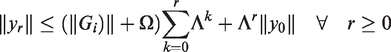
Theorem 3. Consider the hypothesis of Theorem 1, let $\chi :C(E\text{,}{\mathrm{ℝ}}^{N+1})\to C(E\text{,}{\mathrm{ℝ}}^{N+1})$ is the integral operator of equation (10), also $\overline{y}\in C(E\text{,}{\mathrm{ℝ}}^{N+1})$ and the sequence ${\left\{y_r\right\}}_{r\ge 0}$ given in equation (17). Let us also consider $m\in N\text{,}{i}_r\ge 1$ and $\{{\alpha }_0\text{,}{\alpha }_1\text{,}\dots \text{.}\text{.}\text{,}{\alpha }_m\}$ are a set of positive numbers, such that $\forall r\in \{0\text{,}1\text{,}\dots \text{.}\text{,}m\}$ we have

$$\Delta T_{i_r}\le \frac{{\alpha }_r}{2{\rho }_r}\text{,}\Delta T_{j_r}\le \frac{{\alpha }_r}{2{\xi }_r}$$

Then

$$\mathrm{\parallel }\chi (y_{r-1})-y_r\mathrm{\parallel }\le {\alpha }_r$$

(28)

Also, if actual solution of equation (1) is $y$ , then the error $\mathrm{\parallel }y-y_m\mathrm{\parallel }$ is in the form

$$\mathrm{\parallel }y-y_m\mathrm{\parallel }\le \frac{{\Pi }^m}{1-\Pi }\mathrm{\parallel }\chi (\overline{y})-\overline{y}\mathrm{\parallel }+{\displaystyle \sum _{r=0}^m}{\Pi }^{m-r}{\alpha }_r$$

(29)

Proof 3. To prove equation (28), since $t\in E$ and for each $r\in \{0\text{,}1\text{,}\dots \text{,}m\}$ , then by using previous theorem

$$\begin{array}{l}\mathrm{\parallel }\chi y_{r-1}(t)-y_r(t){\mathrm{\parallel }}_{\infty }\\ =\Vert y_0(t)+{\left[{\displaystyle {\int }_0^{t_i}}\left({\sigma }_{r-1\text{,}0}\left(t\text{,}s\right)\right)\text{d}s\text{,}\dots \text{,}{\displaystyle {\int }_0^{t_i}}\left({\sigma }_{r-1\text{,}N}\left(t\text{,}s\right)\right)\text{d}s\right]}^T\\ +{\left[{\displaystyle {\int }_0^{t_i}}\left({\psi }_{r-1\text{,}0}\left(t\text{,}s\right)\right)\text{d}s\text{,}\dots \text{,}{\displaystyle {\int }_0^{t_i}}\left({\psi }_{r-1\text{,}N}\left(t\text{,}s\right)\right)\text{d}s\right]}^T+G_i(t)\\ -(y_0\left(t\right)+{\left[{\displaystyle {\int }_0^{t_i}}{S}_{i_r^2}\left({\sigma }_{r-1\text{,}0}\left(t\text{,}s\right)\right)\text{d}s\text{,}\dots \text{,}{\displaystyle {\int }_0^{t_i}}{S}_{i_r^2}\left({\sigma }_{r-1\text{,}N}\left(t\text{,}s\right)\right)\text{d}s\right]}^T\\ {+{\left[{\displaystyle {\int }_0^{t_i}}{S}_{j_r^2}\left({\psi }_{r-1\text{,}0}\left(t\text{,}s\right)\right)\text{d}s\text{,}\dots \text{,}{\displaystyle {\int }_0^{t_i}}{S}_{j_r^2}\left({\psi }_{r-1\text{,}N}\left(t\text{,}s\right)\right)\text{d}s\right]}^T+G_i\left(t\right))\Vert }_{\infty }\\ \le {\displaystyle {\int }_0^{t_i}}\parallel [{\sigma }_{r-1\text{,}0}\left(t\text{,}s\right)-S_{i_r^2}\left({\sigma }_{r-1\text{,}0}\left(t\text{,}s\right)\right)\text{,}\dots \text{,}\\ \begin{array}{l}{{\sigma }_{r-1\text{,}N}(t\text{,}s)-S_{i_r^2}\left({\sigma }_{r-1\text{,}N}\left(t\text{,}s\right)\right)]\parallel }_{\infty }\mathrm{ds}\\ +{\displaystyle {\int }_0^{t_i}}\parallel [{\psi }_{r-1\text{,}0}(t\text{,}s)-S_{j_r^2}\left({\psi }_{r-1\text{,}0}\left(t\text{,}s\right)\right)\text{,}\dots \text{,}\\ {{\psi }_{r-1\text{,}N}(t\text{,}s)-S_{j_r^2}\left({\psi }_{r-1\text{,}N}\left(t\text{,}s\right)\right)]}^T{\parallel }_{\infty }\mathrm{ds}\end{array}\\ \le {\rho }_r\Delta T_{i_r}+{\xi }_r\Delta T_{j_r}\le {\alpha }_r\end{array}$$

Applying equation (13), then

$$\mathrm{\parallel }y-{\chi }^m(\overline{y})\mathrm{\parallel }\le \frac{{\Pi }^m}{1-\Pi }\mathrm{\parallel }\chi (\overline{y})-\overline{y}\mathrm{\parallel }$$

(30)

Now recursively using equations (12) and (28), then we get

$$\begin{array}{l}\mathrm{\parallel }{\chi }^m(\overline{y})-y_m\mathrm{\parallel }=\mathrm{\parallel }{\chi }^m(y_0)-y_m\mathrm{\parallel }\\ \le {\displaystyle \sum _{r=0}^m}\mathrm{\parallel }{\chi }^{m-r+1}(y_{r-1})-{\chi }^{m-r}(y_r)\mathrm{\parallel }\\ \le {\displaystyle \sum _{r=0}^m}{\Pi }^{m-r}\mathrm{\parallel }\chi (y_{r-1})-y_r\mathrm{\parallel }\le {\displaystyle \sum _{r=0}^m}{\Pi }^{m-r}{\alpha }_r\end{array}$$

(31)

By triangular inequality

$$\mathrm{\parallel }y-y_m\mathrm{\parallel }\le \mathrm{\parallel }y-{\chi }^m(\overline{y})\mathrm{\parallel }+\mathrm{\parallel }{\chi }^m(\overline{y})-y_m\mathrm{\parallel }$$

(32)

putting equations (30) and (31) in equation (32), this is the complete proof.

Numerical test problems

In this section, we perform a number of numerical test problems to show the simplicity and accuracy of the proposed numerical scheme.

Example 1. In the given example, a damped oscillator equation with delay retorting force and external constant force is considered: ¹⁹

$$\{\begin{array}{l}\frac{d^{2}y(t)}{d{t}^2}+\frac{dy(t)}{dt}+y(t-1)=10\text{,}\hfill \\ y(t)=\cos (t)\text{,}\frac{dy(t)}{dt}=-\sin (t)\text{,}t\in [-1\text{,}0]\hfill \end{array}$$

(33)

We can write equation (33) in terms of a linear first order system as follows

$$\left(\begin{array}{c}\frac{d{y}_1(t)}{dt}\\ \frac{d{y}_2(t)}{dt}\end{array}\right)=\left(\begin{array}{cc}0& 1\\ 0& -1\end{array}\right)\left(\begin{array}{c}{y}_1(t)\\ y_2(t)\end{array}\right)+\left(\begin{array}{cc}0& 0\\ -1& 0\end{array}\right)\left(\begin{array}{c}{y}_1(t-1)\\ y_2(t-1)\end{array}\right)+\left(\begin{array}{c}0\\ 10\end{array}\right)$$

(34)

where the initial conditions are $y_1(t):=y(t)=\cos (t)$ and $y_2(t):=\frac{dy(t)}{dt}=-\sin (t)$ .

The exact solutions of equation (34) for $0\le t\le 1$ is

$$\{\begin{array}{l}{y}_1(t)=-\frac{1}{2}\cos (t-1)+\frac{1}{2}\sin (t-1)\hfill \\ -e^{-t}\left(-10-\frac{1}{2}\cos (1)+\frac{1}{2}\sin (1)\right)+10t+\sin (1)-9\hfill \\ y_2(t)=\frac{1}{2}\cos (t-1)+\frac{1}{2}\sin (t-1)\hfill \\ +\hspace{0.17em}{e}^{-t}\left(-10-\frac{1}{2}\cos (1)+\frac{1}{2}\sin (1)\right)+10.\hfill \end{array}$$

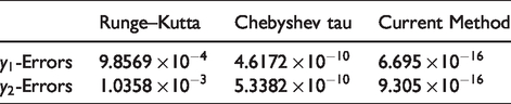
To determined the approximate solution $y_1(t)$ and $y_2(t)$ of the system equation (34) by using LSCM. The absolute error between numerical solution and analytical solution is given in Table 1, and we clearly see that the maximum error of the solution $y_1(t)$ is ${10}^{-15}$ , where the minimum error is ${10}^{-16}$ . Similarly, for $y_2(t)$ the maximum error is ${10}^{-15}$ and minimum error is ${10}^{-16}$ , which is a good agreement between both the solutions. Similarly, to see the convergence of the proposed method we also obtained the error for different values $N=4$ and $N=6$ . The validation of the numerical scheme, in Figure 1 we plotted numerical and analytical solutions $(a):y_1(t)$ and $(b):y_2(t)$ of the system equation (34), which show the efficiency of the present method. The numerical result concede the accuracy of the present method. We also compare the absolute error of the system equation (34) by different methods Runge-Kutta, Chebyshev and current method LSCM in Table 2. From the following comparison we clearly see that the LSCM is more efficient than Runge-Kutta and Chebyshev methods.

Table 1.

Absolute point-wise error of system equation (34).

	$y_1$ -Errors			$y_2$ -Errors
$t_i$	$N=4$	$N=6$	$N=8$	$N=4$	$N=6$	$N=8$
0.0	3.877  $\times {10}^{-6}$	3.077  $\times {10}^{-10}$	1.530  $\times {10}^{-15}$	4.968  $\times {10}^{-6}$	2.015  $\times {10}^{-10}$	1.581  $\times {10}^{-15}$
0.2	4.076  $\times {10}^{-6}$	3.273  $\times {10}^{-10}$	1.115  $\times {10}^{-15}$	4.994  $\times {10}^{-6}$	2.019  $\times {10}^{-10}$	1.217  $\times {10}^{-15}$
0.4	4.137  $\times {10}^{-6}$	3.264  $\times {10}^{-10}$	6.695  $\times {10}^{-16}$	4.998  $\times {10}^{-6}$	2.024  $\times {10}^{-10}$	9.305  $\times {10}^{-16}$
0.6	4.164  $\times {10}^{-6}$	3.172  $\times {10}^{-10}$	8.861  $\times {10}^{-16}$	4.999  $\times {10}^{-6}$	2.106  $\times {10}^{-10}$	1.082  $\times {10}^{-15}$
0.8	4.178  $\times {10}^{-6}$	3.188  $\times {10}^{-10}$	9.335  $\times {10}^{-16}$	4.207  $\times {10}^{-6}$	2.125  $\times {10}^{-10}$	1.039  $\times {10}^{-15}$
1.0	4.186  $\times {10}^{-6}$	3.192  $\times {10}^{-10}$	1.135  $\times {10}^{-15}$	4.264  $\times {10}^{-6}$	2.153  $\times {10}^{-10}$	1.313  $\times {10}^{-15}$

Figure 1.

Comparison both approximate and actual solution of the system equation (34) (a) $y_1(t)$ and (b) $y_2(t)$ .

Table 2.

Comparison of absolute error of system equation (34) for N = 8, refer Mousa-Abadian and Momeni-Masuleh. ¹⁹

	Runge–Kutta	Chebyshev tau	Current Method
$y_1$ -Errors	9.8569  $\times {10}^{-4}$	4.6172  $\times {10}^{-10}$	6.695  $\times {10}^{-16}$
$y_2$ -Errors	1.0358  $\times {10}^{-3}$	5.3382  $\times {10}^{-10}$	9.305  $\times {10}^{-16}$

Figure 2.

Comparison of numerical and exact solution of equation (35).

Example 2. Consider the scalar equation, ⁶ is given by

$$\{\begin{array}{l}\frac{d}{dt}y(t)=-y(t-1)\hfill \\ y(t)=\frac{1}{2}t\text{,}t\in [-1\text{,}0]\hfill \end{array}$$

(35)

In a test model equation (35), $y(t)=\frac{1}{2}t$ is the initial function, where the actual solution of equation (35) is

$$y(t)=-\frac{1}{4}{t}^2+\frac{1}{2}t\text{,}t\in [0\text{,}1]$$

We determine the numerical solution $y(t)$ of equation (35) by LSCM. For the given simulation we can use only $N=8$ number of nodes. The absolute error of both the solutions is given in Table 3, and we see the minimum error is ${10}^{-16}$ . For the convergence of the proposed method, we also obtained the error for different values of $N$ , therefor $N=4$ $N=6$ $N=8$ , $N=12$ , $N=16$ , and $N=20$ . For the validation of Legendre spectral collocation method, we plot both numerical and exact solutions of equation (35) in Figure 2, which shows the efficiency of the present method.

Table 3.

Absolute point-wise error of equation (35).

$t_i$	0.0	0.2	0.4	0.6	0.8	1.0
Error  $N=4$	1.968  $\times {10}^{-6}$	2.271  $\times {10}^{-6}$	2.374  $\times {10}^{-6}$	2.421  $\times {10}^{-6}$	2.446  $\times {10}^{-6}$	2.461  $\times {10}^{-6}$
Error  $N=6$	4.921  $\times {10}^{-10}$	5.677  $\times {10}^{-10}$	5.936  $\times {10}^{-10}$	6.053  $\times {10}^{-10}$	6.115  $\times {10}^{-10}$	6.152  $\times {10}^{-10}$
Error  $N=8$	1.110  $\times {10}^{-16}$	1.072  $\times {10}^{-16}$	1.065  $\times {10}^{-16}$	1.084  $\times {10}^{-16}$	1.075  $\times {10}^{-16}$	1.071  $\times {10}^{-16}$
Error  $N=12$	1.073  $\times {10}^{-16}$	1.066  $\times {10}^{-16}$	1.085  $\times {10}^{-16}$	1.077  $\times {10}^{-16}$	1.073  $\times {10}^{-16}$	1.069  $\times {10}^{-16}$
Error  $N=16$	1.072  $\times {10}^{-16}$	1.065  $\times {10}^{-16}$	1.084  $\times {10}^{-16}$	1.071  $\times {10}^{-16}$	1.067  $\times {10}^{-16}$	1.076  $\times {10}^{-16}$
Error  $N=20$	1.072  $\times {10}^{-16}$	1.065  $\times {10}^{-16}$	1.084  $\times {10}^{-16}$	1.075  $\times {10}^{-16}$	1.071  $\times {10}^{-16}$	1.067  $\times {10}^{-16}$

Table 4.

The absolute point-wise error of equation (36).

	$y_1$ -Errors		$y_2$ -Errors		$y_3$ -Errors
$t_i$	$N=4$	$N=8$	$N=4$	$N=8$	$N=4$	$N=8$
0.0	2.329  $\times {10}^{-6}$	9.869  $\times {10}^{-17}$	1.733  $\times {10}^{-6}$	1.110  $\times {10}^{-16}$	2.329  $\times {10}^{-6}$	2.220  $\times {10}^{-16}$
0.2	2.886  $\times {10}^{-6}$	6.316  $\times {10}^{-17}$	1.733  $\times {10}^{-6}$	1.110  $\times {10}^{-16}$	2.886  $\times {10}^{-6}$	7.944  $\times {10}^{-17}$
0.4	3.085  $\times {10}^{-6}$	1.198  $\times {10}^{-16}$	1.742  $\times {10}^{-6}$	8.983  $\times {10}^{-17}$	3.085  $\times {10}^{-6}$	8.478  $\times {10}^{-17}$
0.6	3.177  $\times {10}^{-6}$	1.294  $\times {10}^{-16}$	1.808  $\times {10}^{-6}$	7.343  $\times {10}^{-17}$	3.177  $\times {10}^{-6}$	4.370  $\times {10}^{-17}$
0.8	3.226  $\times {10}^{-6}$	1.061  $\times {10}^{-16}$	1.831  $\times {10}^{-6}$	9.986  $\times {10}^{-17}$	3.226  $\times {10}^{-6}$	1.328  $\times {10}^{-16}$
1.0	3.255  $\times {10}^{-6}$	6.101  $\times {10}^{-17}$	1.839  $\times {10}^{-6}$	9.029  $\times {10}^{-17}$	3.255  $\times {10}^{-6}$	5.827  $\times {10}^{-17}$

Table 5.

Comparison of absolute error of system equation (36) for N = 8, refer Mousa-Abadian and Momeni-Masuleh. ¹⁹

	Runge–Kutta	Chebyshev tau	Current method
$y_1$ -Errors	6.7972  $\times {10}^{-4}$	6.6613  $\times {10}^{-16}$	7.343  $\times {10}^{-17}$
$y_2$ -Errors	1.9309  $\times {10}^{-3}$	2.2204  $\times {10}^{-16}$	9.986  $\times {10}^{-17}$
$y_3$ -Errors	8.8818  $\times {10}^{-16}$	1.7763  $\times {10}^{-15}$	5.827  $\times {10}^{-17}$

Example 3. Consider the following system ¹⁹

$$\left(\begin{array}{c}\frac{d}{dt}{y}_1(t)\\ \frac{d}{dt}{y}_2(t)\\ \frac{d}{dt}{y}_3(t)\end{array}\right)=\left(\begin{array}{ccc}0& 2& 0\\ 0& 0& -1\\ 0& 0& 0\end{array}\right)\left(\begin{array}{c}{y}_1(t)\\ y_2(t)\\ y_3(t)\end{array}\right)+\left(\begin{array}{ccc}0& 0& 0\\ 1& 0& 0\\ 0& 2& 0\end{array}\right)\left(\begin{array}{c}{y}_1(t-1)\\ y_2(t-1)\\ y_2(t-1)\end{array}\right)$$

(36)

where the initial function is $y_i(t)=1\text{,}-1\le t\le 0$ .

The exact solution of equation (36) for $0\le t\le 1$ is

$$\{\begin{array}{l}{y}_1(t)=-\frac{2}{3}{t}^3+2t+1\text{,}\hfill \\ y_2(t)=1-t^2\text{,}\hfill \\ y_3(t)=1+2t\text{,}\hfill \end{array}$$

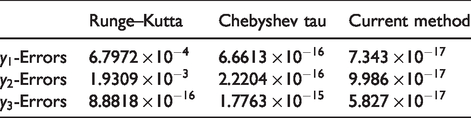
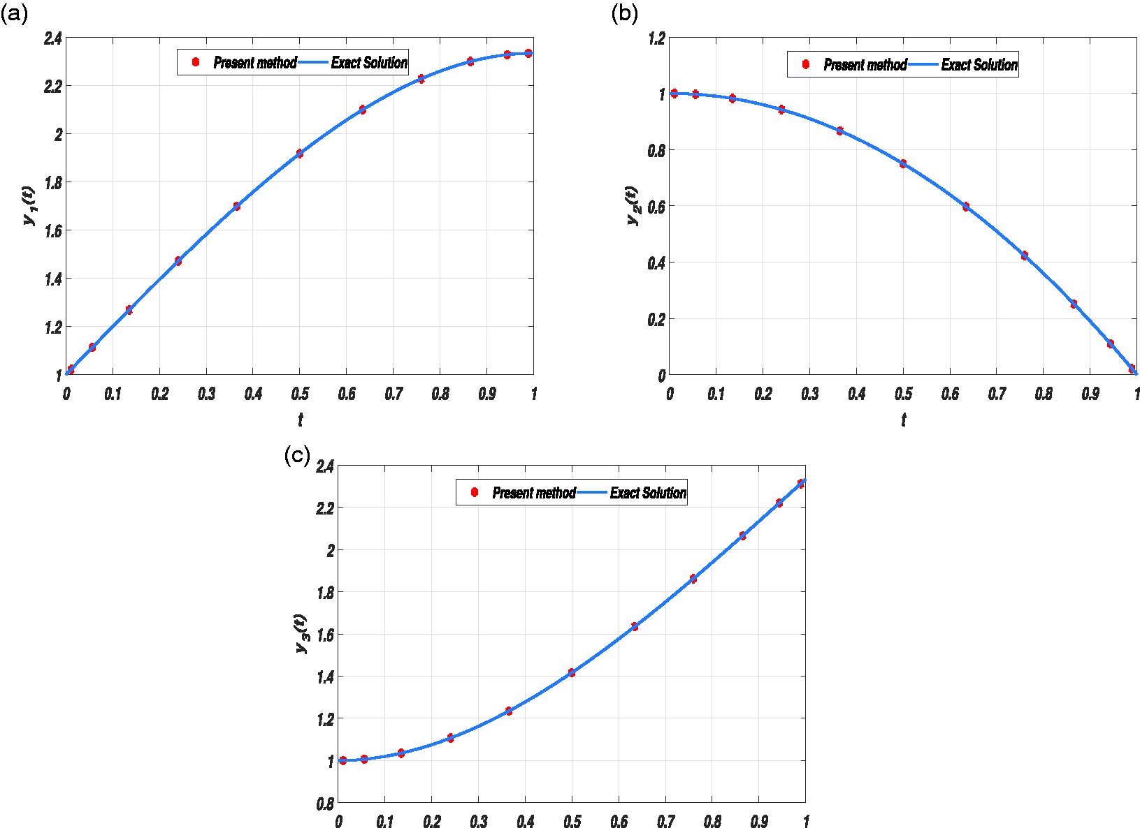
By using proposed numerical scheme LSCM, to determined the numerical solutions $y_1(t)\text{,\hspace{0.17em}}{y}_2(t)$ and $y_3(t)$ of system equation (36). The absolute error between analytical and numerical solution is shown in Table $4$ . Since for only $N=8$ number of nodes the maximum error of the solution system equation (36) is ${10}^{-16}$ , where the minimum error is ${10}^{-11}$ which are clearly shown in columns $2\text{,\hspace{0.17em}}3$ , and $4$ of Table 3. Similarly, for the convergence of the Legendre spectral collocation method, we also obtained the error for $N=4$ . The numerical and analytical solution of the system equation (36) $(a):y_1(t)\text{,}(b):y_2(t)$ and $(c):y_3(t)$ are plotted in Figure 3, and we clearly see that both the solution are in their good agreements. Once again we compare the absolute error of the system equation (36) by Runge-Kutta, Chebyshev and LSCM in Table 5. From the following comparison we clearly see that the LSCM is more efficient than Runge-Kutta and Chebyshev methods.

Figure 3.

Comparison of the solutions of system equation (36) where (a) $y_1(t)$ , (b) $y_2(t)$ and (c) $y_3(t)$ .

Figure 4.

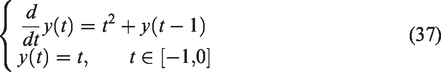
Both the approximate and actual solution of equation (37).

Example 4. Consider the scalar equation ⁶ given by

$$\{\begin{array}{c}\frac{d}{dt}y(t)=t^2+y(t-1)\\ y(t)=t\text{,}t\in [-1\text{,}0]\end{array}$$

(37)

In equation (37), $y(t)=t$ is initial function, where the exact solution for $0\le t\le 1$ is given by

$$y(t)=\frac{1}{3}{t}^3+\frac{1}{2}{t}^2-t$$

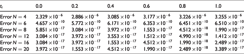
We determine the numerical solution $y(t)$ of equation (37) by LSCM. The absolute error between analytical and numerical solution is given in Table 6 and we see that the minimum error is ${10}^{-16}$ , using $N=8$ numbers of nodes. Similarly, for the convergence of the proposed method we also obtained the error for different values of $N$ , therefor $N=4$ $N=6$ $N=8$ , $N=12$ , $N=16$ , and $N=20$ . For the validation of the proposed LSCM, both the numerical and analytical solutions of equation (37) are plotted in Figure 4, which shows the accuracy of LSCM.

Table 6.

The absolute point-wise error of equation (37).

$t_i$	0.0	0.2	0.4	0.6	0.8	1.0
Error  $N=4$	7.873  $\times {10}^{-7}$	9.084  $\times {10}^{-7}$	9.498  $\times {10}^{-7}$	9.684  $\times {10}^{-7}$	9.783  $\times {10}^{-7}$	9.842  $\times {10}^{-7}$
Error  $N=6$	1.575  $\times {10}^{-10}$	1.817  $\times {10}^{-10}$	1.900  $\times {10}^{-10}$	1.937  $\times {10}^{-10}$	1.957  $\times {10}^{-10}$	1.968  $\times {10}^{-10}$
Error  $N=8$	1.072  $\times {10}^{-16}$	1.094  $\times {10}^{-16}$	1.084  $\times {10}^{-16}$	1.093  $\times {10}^{-16}$	1.086  $\times {10}^{-16}$	1.073  $\times {10}^{-16}$
Error  $N=12$	1.073  $\times {10}^{-16}$	1.095  $\times {10}^{-16}$	1.085  $\times {10}^{-16}$	1.094  $\times {10}^{-16}$	1.087  $\times {10}^{-16}$	1.083  $\times {10}^{-16}$
Error  $N=16$	1.095  $\times {10}^{-16}$	1.085  $\times {10}^{-16}$	1.096  $\times {10}^{-16}$	1.087  $\times {10}^{-16}$	1.089  $\times {10}^{-16}$	1.084  $\times {10}^{-16}$
Error  $N=20$	3.084  $\times {10}^{-16}$	1.094  $\times {10}^{-16}$	1.087  $\times {10}^{-16}$	1.083  $\times {10}^{-16}$	1.089  $\times {10}^{-16}$	1.084  $\times {10}^{-16}$

Example 5. Consider the scalar equation, ⁶ is given by

$$\{\begin{array}{l}\frac{d}{dt}y(t)=y(t-1)+y\left(t-\frac{1}{2}\right)\hfill \\ y(t)=\frac{t}{2}\text{,}t\in [-1\text{,}0]\hfill \end{array}$$

(38)

In equation (38), the initial function is $y(t)=\frac{1}{2}t$ , where exact solution for $0\le t\le 1$ of equation (38) is given by

$$y(t)=\{\begin{array}{l}\frac{1}{2}{t}^2+\frac{3}{4}t\text{,}0\le t\le \frac{1}{2}\hfill \\ \frac{1}{6}{\left(t-\frac{1}{2}\right)}^3-\frac{3}{8}{\left(t-\frac{1}{2}\right)}^2+\frac{1}{4}{(t-1)}^2-\frac{5}{16}\text{,}\frac{1}{2}\le t\le 1\hfill \end{array}$$

Once again, to determine the approximate solution $y(t)$ of equation (38) by LSCM. The absolute error between analytical and numerical simulation is given in Table 7, we see that the maximum error is ${10}^{-17}$ . Similarly, for the convergence of the Legendre spectral collocation method we also obtained the error for different values of $N$ , therefor $N=4$ $N=6$ $N=8$ , $N=12$ , $N=16$ , and $N=20$ . The comparison of the numerical and analytical solutions of equation (38) is plotted in Figure 5, which shows the efficiency of the present method. For the given simulation we can use $N=8$ nodes.

Table 7.

The absolute point-wise error of equation (38).

$t_i$	0.0	0.2	0.4	0.6	0.8	1.0
Error  $N=4$	2.329  $\times {10}^{-6}$	2.886  $\times {10}^{-6}$	3.085  $\times {10}^{-6}$	3.177  $\times {10}^{-6}$	3.226  $\times {10}^{-6}$	3.255  $\times {10}^{-6}$
Error  $N=6$	4.657  $\times {10}^{-10}$	5.772  $\times {10}^{-10}$	6.171  $\times {10}^{-10}$	6.353  $\times {10}^{-10}$	6.451  $\times {10}^{-10}$	6.510  $\times {10}^{-10}$
Error  $N=8$	5.851  $\times {10}^{-17}$	3.084  $\times {10}^{-17}$	3.972  $\times {10}^{-17}$	1.553  $\times {10}^{-17}$	4.512  $\times {10}^{-18}$	1.990  $\times {10}^{-17}$
Error  $N=12$	3.084  $\times {10}^{-17}$	3.972  $\times {10}^{-17}$	3.553  $\times {10}^{-17}$	1.512  $\times {10}^{-17}$	4.990  $\times {10}^{-18}$	1.412  $\times {10}^{-17}$
Error  $N=16$	3.084  $\times {10}^{-17}$	3.972  $\times {10}^{-17}$	1.553  $\times {10}^{-17}$	4.512  $\times {10}^{-17}$	1.990  $\times {10}^{-18}$	2.489  $\times {10}^{-17}$
Error  $N=20$	3.972  $\times {10}^{-17}$	1.553  $\times {10}^{-17}$	4.512  $\times {10}^{-17}$	1.990  $\times {10}^{-17}$	2.489  $\times {10}^{-18}$	3.389  $\times {10}^{-17}$

Figure 5.

Both the approximate and actual solution of equation (38).

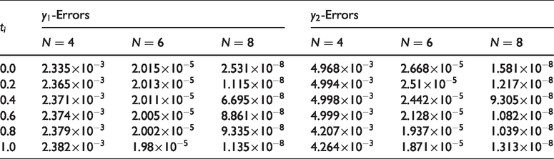
Example 6. Consider the following nonlinear system of DDEs, ³⁰ is given by

$$\begin{array}{l}\frac{d{y}_1(t)}{dt}=a{y}_1(t)+b{y}_2(t)+c\frac{y_1(t-1)}{1+y_1^2(t-1)}+g_1(t)t>0\\ \frac{d{y}_2(t)}{dt}=b{y}_1(t)+a{y}_2(t)+c\frac{y_2(t-1)}{1+y_2^2(t-1)}+g_2(t)t\le 0\end{array}$$

(39)

We assume the following analytical solution for the equation (39) for the initial conditions $y_1(t)=0$ and $y_2(t)=-2$ are

$$\begin{array}{l}{y}_1(t)=2(\sin 2\pi t+\cos 2\pi t)\text{,}\\ y_2(t)=2(\sin 2\pi t-\cos 2\pi t)\end{array}$$

(40)

With the functions $g_1(t)$ and $g_2(t)$ are given by

$$\begin{array}{l}{g}_1(t)=\frac{\left\{\frac{(2((35+6\pi )\cos 2\pi t+2(-5+2\pi )\cos 6\pi t}{+(29-6\pi )\sin 2\pi t+2(7+2\pi )\sin 6\pi t))}\right\}}{5+4\sin 4\pi t}\\ g_2(t)=\frac{\left\{\frac{(2((-35+6\pi )\cos 2\pi t+2(5+2\pi )\cos 6\pi t}{+(29+6\pi )\sin 2\pi t+2(7-2\pi )\sin 6\pi t))}\right\}}{5-4\sin 4\pi t}\end{array}$$

(41)

The Legendre spectral collocation method is applied to this example with values of the parameters as $a=-6\text{,\hspace{0.17em}}b=1\text{,\hspace{0.17em}}c=10$ and $0\le t\le 1$ . The numerical results are reported in Table 8. In order to obtain the convergence of the proposed method, we have obtains the result for different number of nodes like $N=4$ , $N=6$ , and $N=8$ . The performance of the proposed method is good as compared with other examples. Both the numerical and analytical solution are shown in Figure 6. The given system are also numerically solved by author in Li and Zhang ³⁰ using Broydens method, which has achieve only ${10}^{-2}$ accuracy using $N=64$ .

Table 8.

Absolute point-wise error of system equation (39).

$t_i$	$y_1$ -Errors			$y_2$ -Errors
	$N=4$	$N=6$	$N=8$	$N=4$	$N=6$	$N=8$
0.0	2.335 $\times {10}^{-3}$	2.015 $\times {10}^{-5}$	2.531 $\times {10}^{-8}$	4.968 $\times {10}^{-3}$	2.668 $\times {10}^{-5}$	1.581 $\times {10}^{-8}$
0.2	2.365 $\times {10}^{-3}$	2.013 $\times {10}^{-5}$	1.115 $\times {10}^{-8}$	4.994 $\times {10}^{-3}$	2.51 $\times {10}^{-5}$	1.217 $\times {10}^{-8}$
0.4	2.371 $\times {10}^{-3}$	2.011 $\times {10}^{-5}$	6.695 $\times {10}^{-8}$	4.998 $\times {10}^{-3}$	2.442 $\times {10}^{-5}$	9.305 $\times {10}^{-8}$
0.6	2.374 $\times {10}^{-3}$	2.005 $\times {10}^{-5}$	8.861 $\times {10}^{-8}$	4.999 $\times {10}^{-3}$	2.128 $\times {10}^{-5}$	1.082 $\times {10}^{-8}$
0.8	2.379 $\times {10}^{-3}$	2.002 $\times {10}^{-5}$	9.335 $\times {10}^{-8}$	4.207 $\times {10}^{-3}$	1.937 $\times {10}^{-5}$	1.039 $\times {10}^{-8}$
1.0	2.382 $\times {10}^{-3}$	1.98 $\times {10}^{-5}$	1.135 $\times {10}^{-8}$	4.264 $\times {10}^{-3}$	1.871 $\times {10}^{-5}$	1.313 $\times {10}^{-8}$

Figure 6.

Comparison of both approximate and actual solution of the system equation (39) (a) $y_1(t)$ and (b) $y_2(t)$ .

Conclusion

It has been the aim of this article to apply an efficient and reliable numerical technique for the approximate solution to a system of time DDEs. To this end, we apply a numerical technique based on Legendre spectral collocation method. A rigorous error and convergence analysis were performed for the proposed numerical scheme. A number of numerical experiments were performed to confirm the theoretical exponential rate of convergence. We also consider a nonlinear time delay system and find their numerical solution by proposed method. The obtained results were compare with the exact solution and with the other available numerical technique. It is found that our scheme has a very good agreement with the exact solution as well as with other available numerical schemes.