Sage Journals: Discover world-class research

Abstract

Bearings are the core components of ship propulsion shafting, and effective prediction of their working condition is crucial for reliable operation of the shaft system. Shafting vibration signals can accurately represent the running condition of bearings. Therefore, in this article, we propose a new model that can reliably predict the vibration signal of bearings. The proposed method is a combination of a fuzzy-modified Markov model with gray error based on particle swarm optimization (PGFM (1,1)). First, particle swarm optimization was used to optimize and analyze the three related parameters in the gray model (GM (1,1)) that affect the data fitting accuracy, to improve the data fitting ability of GM (1,1) and form a GM (1,1) based on particle swarm optimization, which is called PGM (1,1). Second, considering that the influence of historical relative errors generated by data fitting on subsequent data prediction cannot be expressed quantitatively, the fuzzy mathematical theory was introduced to make fuzzy corrections to the historical errors. Finally, a Markov model is combined to predict the next development state of bearing vibration signals and form the PGFM (1,1). In this study, the traditional predictions of GM (1,1), PGM (1,1), and newly proposed PGFM (1,1) are carried out on the same set of bearing vibration data, to make up for the defects of the original model layer by layer and form a set of perfect forecast system models. The results show that the predictions of PGM (1,1) and PGFM (1,1) are more accurate and reliable than the original GM (1,1). Hence, they can be helpful in the design of practical engineering equipment.

Keywords

Particle swarm optimization algorithm gray system theory fuzzy mathematical theory Markov data forecasting shafting vibration

Introduction

Bearings are among the components most commonly used and most prone to failure in marine propulsion shafting. Their working state can directly affect reliable navigation of the ship. Accordingly, accurate early warnings of bearing degradation can help decision-makers to formulate appropriate measures to avoid accidents. Liu¹ proposed a bearing life prediction method based on the Weibull proportional hazard model (WPHM). This method predicts the root mean square (RMS) and kurtosis of bearing vibration signals, which can represent various failure modes of bearings,² and uses them as covariates in the WPHM to predict the remaining lifetime of the bearing. Therefore, the establishment of a robust and accurate model to predict the characteristic quantities of bearing vibration, to improve the prediction of bearing life, has become a critical task. Many prediction methods based on big data have been studied and applied, including neural networks and support vector machines. However, the implementation of these methods requires a large amount of initial data as support. Moreover, because of the working environment of marine propulsion shaft bearings, it is not realistic to obtain a large amount of bearing vibration data. Therefore, a method that can predict data from a small amount of initial data is crucial.

The gray theory was first proposed by Professor Deng³ in 1982. The gray model (GM (1,1)) is the most important model in gray prediction theory and has led to many achievements in prediction. Different from the general prediction methods based on a large amount of historical data, GM (1,1) can find internal rules from a small number of data sequences containing random numbers and random disturbances. This allows more practical analyses and predictions by starting from the signal itself. Although GM (1,1) has been widely adopted in recent years, its predictive performance needs to be further improved. Optimization and upgrading operations of GM (1,1) have been carried out by many experts and scholars worldwide. These operations can be roughly divided into three types. In the first type, algorithms are used to perform optimization calculations on the parameters of GM (1,1) itself to improve the prediction accuracy.^4–6 In the second type, the data processing mode of the model itself is improved according to different forms of the sequence of objects (monotone, oscillation, dispersion, etc.).^7–10 In the third type, GM (1,1) is combined with another reliable theoretical model to overcome the shortcomings of GM (1,1) and improve its prediction accuracy.^11–13 However, these strategies have some shortcomings. In the first strategy, the parameters to be optimized are often not fully considered, and the influence of historical errors on subsequent data prediction is not considered. The second strategy has poor generalization ability and can only be used for special data sets. The third strategy does not integrate the advantages of the first and second strategies and does not systematically combine the existing optimization methods.

Based on the above issues, we address the following points in this study:

Because the final mathematical prediction model of GM (1,1) involves three parameters (initial conditions $x^{(0)} (1)$ , development coefficient a, and gray action b), we use the particle swarm optimization (PSO) algorithm to optimize all three parameters.¹⁴ The optimization order is also discussed, and the reasons for the influence of different optimization orders on the prediction accuracy of GM (1,1) are analyzed to form a GM based on PSO, which is named PGM (1,1).

Considering the influence of historical relative errors generated by unfitted unit prediction data on the final prediction value in the process of sequential training of GM (1,1), the influence is fuzzy and cannot be expressed by a quantitative relation.¹⁵ Therefore, we introduce the theory of fuzzy mathematics to deal with the historical error generated by GM (1,1) prediction.

The object studied by the system is always developing and changing, and the effects of external factors on the system are uncertain. The Markov model is suitable for the prediction of random state transition processes in economics, passenger, desert, microorganism, and other objects with irregular development.^16–20 Therefore, the Markov model is combined with GM (1,1) to compensate for the defects of gray prediction theory in the processing of data with large jump.²¹

Therefore, GM (1,1) is selected in this study as the basis of the combined model. First, the PSO algorithm was used to iteratively optimize the three parameters of GM (1,1) to form PGM (1,1). Second, fuzzy mathematical theory was used to fuzzy-correct the prediction data error of PGM (1,1). Finally, by combination with the Markov model to predict the next data state, a new combination prediction model called the PGFM (1,1) was developed. The new combined model can be used to predict the RMS data of bearing vibrations. The data prediction results show that the new model has better prediction ability of the development trend of ships bearing vibration signal characteristic quantities and can provide reliable data for relevant decision-makers.

The rest of this article is organized as follows: Section “Methodology” introduces relevant algorithms and theories involved in PGFM (1,1), including GM (1,1), PSO algorithm, fuzzy mathematical theory, and Markov model. Section “PGFM (1,1) combined model” describes the specific calculation flow of the PGFM (1,1) method. An empirical study is described in section “Empirical study”. Finally, the corresponding discussions and conclusions of this study are given in section “Conclusion”.

Methodology

In this section, all relevant models and theories involved in the newly proposed PGFM (1,1) are introduced, including the gray prediction model GM (1,1), PSO algorithm, fuzzy mathematical theory, and Markov model.

Standard GM (1,1) model

GM (1,1) has a significant effect on the data prediction of the gray system. Its features of simple modeling, small demand for data samples, and easy solution have led to its application in an increasing number of engineering fields.²²

The calculation process of GM (1,1) is shown in Figure 1.

Figure 1.

Calculation flow of traditional GM (1,1).

Step 1: Set the original data sequence to $x^{(0)} = [x^{(0)} (1), x^{(0)} (2), . . ., x^{(0)} (n)]$ . To predict the future development trend and strengthen the data regularity, generate the first-order accumulation sequence $x^{(1)} = [x^{(1)} (1), x^{(2)} (2), . . ., x^{(1)} (n)]$ . The following data sequence $x^{(1)} (i)$ is expressed as

x^{(1)} (k) = \sum_{i = 1}^{k} x^{(0)} (i), k = 1, 2, . . ., n

(1)

Step 2: The generation number of adjacent values based on the first-order accumulation generation sequence is established as follows

z^{(1)} (k) = α x^{(1)} (k) + (1 - α) x^{(1)} (k - 1), k = 2, 3, . . ., n

(2)

where $α$ is the equal weight adjacent value generator (mean generator) and is generally equal to 0.5. Then

z^{(1)} (k) = 0.5 x^{(1)} (k) + 0.5 x^{(1)} (k - 1), k = 2, 3, . . ., n

(3)

Step 3: The gray differential equation of the gray modeling is defined as

x^{(0)} (k) + a z^{(1)} (k) = b or {\begin{matrix} x^{(0)} (2) + a z^{(1)} (2) = b, \\ x^{(0)} (3) + a z^{(1)} (3) = b, \\ \dots \\ x^{(0)} (n) + a z^{(1)} (n) = b \end{matrix}

(4)

where a is the development coefficient and b is the gray action quantity, both of which are the parameters to be calculated.

Into matrix representation

Y = Bu

Y = [\begin{matrix} x^{(0)} (2) \\ x^{(0)} (3) \\ ⋮ \\ x^{(0)} (n) \end{matrix}] B = [\begin{matrix} - z^{(1)} (2) 1 \\ - z^{(1)} (3) 1 \\ ⋮ \\ - z^{(1)} (n) 1 \end{matrix}] u = [\begin{matrix} a \\ b \end{matrix}]

(5)

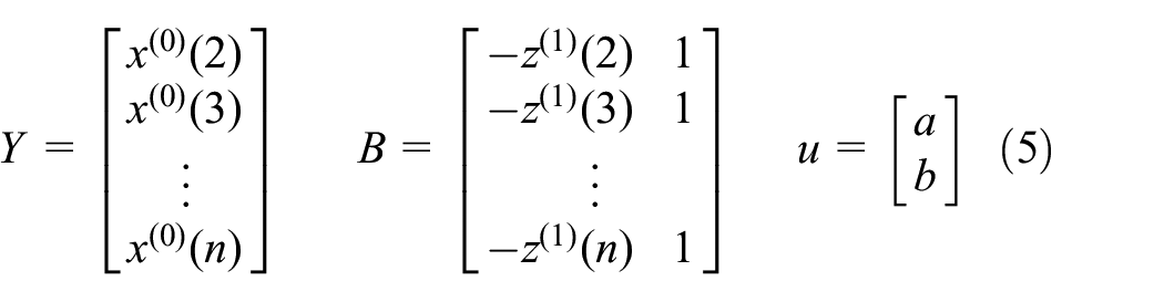
Parameters a and b are obtained by least-square fitting as follows

\hat{u} = [\begin{matrix} \hat{a} \\ \hat{b} \end{matrix}] = (B^{T} B)^{- 1} B^{T} Y

(6)

Step 4: We express the white equation (shadow equation) corresponding to the gray differential equation of the gray prediction model as follows

\frac{d x^{(1)} (t)}{dt} + a x^{(1)} (t) = b

(7)

Solving equation (7), we obtain

x^{(1)} (t) = (x^{(0)} (1) - \frac{b}{a}) e^{- a (t - 1)} + \frac{b}{a}

(8)

Then, we express equation (8) in discrete form as follows

x^{(1)} (k + 1) = (x^{(0)} (1) - \frac{b}{a}) e^{- ak} + \frac{b}{a}

(9)

Step 5: Finally, the predicted value of GM is obtained by subtracting the previous number from each layer as follows

\begin{matrix} {\hat{x}}^{(0)} (k + 1) = x^{(1)} (k + 1) - x^{(1)} (k) \\ = (1 - e^{a}) (x^{(0)} (1) - \frac{b}{a}) e^{- ak} \end{matrix}

(10)

PSO

PSO is essentially a random search algorithm and belongs to the area of emerging intelligent optimization technology. It is an efficient parallel search method with good generality and a reasonable number of preset variables. Its working principle is shown in Figure 2.

Figure 2.

Updating mode of particle swarm location in each generation.

In the PSO, the potential solution of each optimization problem is referred to as “particle,” whose fitness is determined by the optimized function. Each particle has a “velocity,” which determines its optimal direction and distance; the solution is obtained by following the current optimal particle. The main operation of the algorithm is to update the particle velocity and position according to equations (11) and (12) and gradually converge to the ideal position of the objective function²³

v_{t + 1} = w \times v_{t} + c_{1} r_{1} \times (pBest - X_{t}) + c_{2} r_{2} \times (gBest - X_{t})

(11)

X_{t + 1} = X_{t} + V_{t + 1}

(12)

In equations (11) and (12), c is the learning factor (acceleration constant), r is a uniformly random number [0,1], and w is the inertia weight.

The meanings of the terms of equation (11) are briefly described in Figure 2. The first term represents the inertia, which indicates the tendency of a particle to maintain its previous state of motion; the second term represents the self-cognition, which indicates the tendency of a particle to move toward its best position according to historical data; and the third term represents the social cognition, which indicates the tendency of particles to cooperate with each other to move back to the optimal group or adjacent location.

Fuzzy mathematical theory

The concept of fuzzy recognition was proposed long before the appearance of fuzzy mathematics. Its objective is to determine the type of recognized object on the premise that various standard types are known. Fuzzy recognition consists of three steps: extracting features, establishing membership functions, and establishing recognition criteria.²⁴ We define the value range of the data as U and conduct fuzzy state divisions $s_{1}, s_{2}, . . ., s_{n}$ . If $\forall u \in U$

\sum_{m = 1}^{M} μ_{sm} (u) = 1

(13)

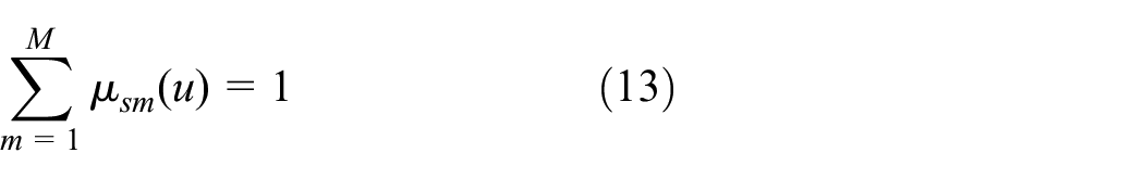
where $μ_{sm} (u)$ is the membership degree of the numerical value u to the fuzzy state $s_{m}$ and is also known as the distribution coefficient of u to $s_{m}$ .

Markov

The core of Markov prediction theory is the establishment of the state transition probability matrix $(P_{ij})_{N \times N}$ . When the amount of data is large, the n-step transition probability matrix can be created. However, for large machinery (such as ship propulsion shafting), the data are relatively small and difficult to collect. Therefore, it is reasonable to create a one-step Markov state transition matrix based on a small amount of data. The time parameter of the data sequence is $t_{1}, t_{2}, . . ., t_{n}$ . When $t = t_{n}$ , the variable $X (t_{n})$ can take the states $a_{1}, a_{2}, . . ., a_{N}$ . If $X_{n - 1} = a_{i}$ , the probability of occurrence of $X_{n} = a_{j}$ in the n = 1 transition is independent of the order “n,” and $P_{ij} = P {X_{n} = a_{j} | X_{n - 1} = a_{i}} (i, j = 1, 2, . . ., N)$ is the (one-step) transition probability of Markov prediction. The corresponding state transition probability matrix is

P = [\begin{matrix} P_{00} (n) P_{01} (n) \dots \\ ⋮ ⋮ ⋮ \\ P_{n 0} (n) P_{n 1} (n) \dots \end{matrix}]

(14)

PGFM (1,1) combined model

The standard GM (1,1) has some error in the data fitting prediction, which is mainly attributed to the insufficient accuracy and rationality of parameter selection in the prediction model. Accordingly, a parameter optimization method (the PSO algorithm) is introduced to iteratively optimize the “problem parameters” in the standard GM (1,1) to form the PGM (1,1). Subsequently, because there remain relative errors of different sizes between the predicted and actual values of PGM (1,1) and because the influence of historical errors on subsequent data prediction cannot be expressed quantitatively, fuzzy mathematical theory is introduced to deal with the influence of historical errors. Finally, because GM (1,1) is suitable for sequences with obvious changing trends and has a poor effect on data with large random volatility, a Markov model is applied for the prediction of state transition behavior of random processes, which makes up for the defect of GM (1,1), introduces the complementary advantages of the two theories,^25,26 and forms the PGFM (1,1). The PGFM (1,1) workflow is shown in Figure 3.

Figure 3.

Flowchart of PGFM (1,1).

The specific operations of PGFM (1,1) are as follows:

Step 1: The standard GM (1,1) predictive mathematical model is established according to the procedure described in section “Standard GM (1, 1) model.”

Step 2: PSO is used to optimize the initial conditions $x^{(0)} (1)$ and parameters a and b in GM (1,1) successively; then, $x^{(0)} (1)$ , a, and b are input in the original formula, and PGM (1,1) is developed. (The reason for the optimization order is explained in section “PGM (1,1) calculation and analysis.”)

Step 3: The relative errors between the actual data and the predicted data fitted by PGM (1,1) are calculated to obtain the data error sequence $e_{i} = [e_{1}, e_{2}, . . ., e_{n}]$ .

Step 4: The value range $e_{i} \in U$ of the error sequence $e_{i}$ is defined, and the fuzzy state division $s_{1}, s_{2}, . . ., s_{n}$ is performed.

Step 5: The fuzzy state transfer coefficient from state $t_{k}$ to states $t_{k + 1}$ , $s_{i}$ , and $s_{j}$ is $μ_{si} (X (t_{k})) \times μ_{sj} (X (t_{k + 1}))$ . The fuzzy transition frequency $A_{ij}$ is

A_{ij} = \sum_{k = 1}^{n - 1} μ_{si} (X (t_{k})) \times μ_{sj} (X (t_{k + 1}))

(15)

Step 6: The fuzzy state transition frequency $A'_{ij}$ is calculated, and the fuzzy state transition probability matrix P is formulated

A'_{ij} = \frac{A_{ij}}{A_{i 1} + A_{i 2} + \dots A_{iM}} = \frac{A_{ij}}{\sum_{j = 1}^{M} A_{ij}}, i, j = 1, 2, . . ., M

(16)

P = [\begin{matrix} {A'}_{11} {A'}_{12} \dots \\ ⋮ ⋮ ⋮ \\ {A'}_{n 1} {A'}_{n 2} \dots \end{matrix}]

(17)

Step 7: With the final time variable $u_{k}$ , the final state fuzzy vector is obtained

S = (s_{1} (u_{k}), s_{2} (u_{k}), . . ., s_{M} (u_{k}))

(18)

Step 8: The fuzzy vector B and fuzzy correction $σ$ of the relative error are calculated as follows

B = S \times P

(19)

σ = B \times M_{si}

(20)

where $M_{si}$ is the intermediate value of fuzzy state $s_{i}$ .

Step 9: Finally, the predicted value of the next state after error correction is obtained as follows

{\hat{x}}^{(0)}^{*} (n + 1) = \frac{{\hat{x}}^{(0)} (n + 1)}{1 + σ}

(21)

Empirical study

Accurate and reliable prediction of the bearing vibration characteristic quantity provides data that support decision-makers to develop both maintenance plans and early warnings of the deterioration of the bearing running state, preventing unnecessary economic losses. Therefore, the development of an accurate, efficient, and robust forecasting method is important. In this section, the results of the predictive analyses performed with GM (1,1), PGM (1,1), and PGFM (1,1) with the same set of data are reported, and their advantages and disadvantages are discussed.

GM (1,1) analysis

The RMS of bearing vibration signals is usually considered an indicator of bearing life, because it can comprehensively and accurately reflect the trend of bearing life degradation. In addition, the traditional gray prediction model has been widely used in the field of engineering data prediction. To verify the effectiveness of GM (1,1) in the prediction of the bearing decay performance index, we consider 10 sets of data (bearing vibration signals’ RMS) from the full-lifecycle degradation experiment of bearings reported in Liao et al.² In this experiment, an acceleration sensor with model DYTRAN 3035B, sensitivity of 100 mV/g, and measuring range of 50 g was used to conduct signal sampling at equal time intervals in a sampling environment with a sampling frequency of 25.6 kHz and a sampling time of 0.1 s through the data acquisition card NIDAQ. The RMS values of 10 sets of bearing vibration signals were obtained as follows

X_{rms} = \sqrt{\frac{\sum_{i = 1}^{N} x_{i}^{2}}{N}}

(22)

The RMS values of the 10 sets obtained were 0.3234, 0.3715, 0.5032, 0.5982, 0.7145, 0.9035, 1.0385, 1.0772, 1.3093, and 1.5239. The first nine sets of data were taken as the original input data of GM (1,1), and the 10th set was used for model validation. Based on the operation steps of GM (1,1), gray modeling was carried out to obtain the gray prediction mathematical model

{\hat{x}}^{(0)} (k + 1) = (1 - e^{- 0.1575}) [0.3234 + \frac{0.3581}{0.1575}] e^{0.1575 k}

(23)

The mathematical model was used for data prediction and fitting, and the obtained data were compared with the experimental data, as shown in Table 1. It can be seen that the GM can be applied to the prediction and calculation of the RMS of the vibration signals, which are indicators of bearing decay. However, its prediction effect is not sufficient and produces large errors.

Table 1.

RMS data predicted by traditional GM (1,1).

Data distribution mode	Serial no.	Actual RMS (g)	GM (1,1) prediction value (g)	Relative error (%)
Training set	1	0.3234	0.3234	0.00
	2	0.3715	0.4430	19.24
	3	0.5032	0.5186	3.05
	4	0.5982	0.6070	1.48
	5	0.7145	0.7106	−0.54
	6	0.9035	0.8319	−7.93
	7	1.0385	0.9738	−6.23
	8	1.0772	1.1399	5.83
	9	1.3093	1.3345	1.92
Test set	10	1.5239	1.5621	2.51
Mean relative error (%)		4.873

RMS: root mean square; GM: gray model.

PGM (1,1) calculation and analysis

The traditional method for the calculation of the parameters of GM (1,1) is too simple, and its accuracy, reliability, and robustness are insufficient. In this section, the “two-step” iterative optimization of the initial conditions $x^{(0)} (1)$ and parameters a and b in GM (1,1) by the PSO algorithm is analyzed, and the problem of prioritization of the optimization order is discussed and analyzed.

PGM (1,1) calculation

Equation (10) is the final prediction expression of the data of GM (1,1). Through observation, it can be concluded that this equation only contains three parameters (initial conditions $x^{(0)} (1)$ , development coefficient a, and gray action b). Therefore, these three parameters are taken as PSO objects that affect the fitting degree of GM (1,1). For the selection of the initial conditions $x^{(0)} (1)$ , the traditional GM (1,1) takes the first number of the original sequence as the initial condition for data fitting; however, many studies have shown that this is not accurate.^27–29 The fitting curve does not necessarily cross this point, and these data are the oldest, which are not closely related to future data. The parameters a and b depend on the original sequence and background value, in which the original sequence cannot be changed. The influence generated by the selection of background value is finally reflected in parameters a and b, so the final analysis of these parameters is relatively practical and effective. Considering that the selection of initial conditions $x^{(0)} (1)$ and the calculation of parameters a and b are independent of each other, a “two-step” iterative optimization method for these three parameters is proposed in this study.

The minimum sum of the squares of the difference between the error of the fitting data and the actual data is taken as the fitness function of PSO: $min [Z (x^{(0)} (1), a, b)] = min [\sum_{i = 1}^{n} {(| {\hat{x}}^{(0)} (i) - x^{(0)} (i) |)}^{2}]$ . To evaluate the accuracy and effectiveness of the two PSO sequences, considering the low complexity of the objective function and the small number of parameters to be optimized, we selected the following optimization environment based on relevant experience (Table 2).

Table 2.

PSO algorithm parameter settings.

Parameter	$N_{max}$	popsize	$N_{c}$	$ε$	w	$c_{1}$	$c_{2}$
Value	500	50	50	$1 E - 10$	$0.6 < w < 0.8$	2	2

$N_{max}$ : maximum iteration number; popsize: population size; $N_{c}$ : minimum number of iterations; $ε$ : convergence accuracy; w, $c_{1}$ , and $c_{2}$ : parameters of the velocity update formula.

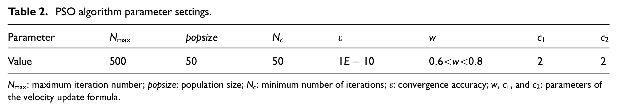
In this environment, the optimization calculation is carried out as follows:

Optimization order 1: With $x^{(0)} (1) = 0.3234$ , PSO is performed to calculate the parameters a and b iteratively; the optimal values of parameters a and b are approximately $a'_{1} = - 0.1576$ and $b'_{1} = 0.3561$ , respectively. Then, the initial conditions $x^{(0)} (1)$ are optimized through the obtained parameters $a'_{1}$ and $b'_{1}$ , and the initial conditions are approximately $x_{1}^{(0)'} (1) = 0.3242$ . Therefore, the optimized gray prediction model can be expressed as

{\hat{x}}_{1}^{(0)} (k + 1) = (1 - e^{- 0.1576}) [0.3242 - \frac{0.3561}{- 0.1576}] e^{0.1576 k}

(24)

Optimization order 2: With the original parameters of the traditional GM a and b, PSO is performed to iteratively optimize the initial condition $x^{(0)} (1)$ and obtain the optimal value of $x_{2}^{(0)'} (1) = 0.3115$ . Then, optimized parameters $a'_{2} = - 0.1576$ and $b'_{2} = 0.3580$ are obtained by using the optimized initial conditions $x_{2}^{(0)'} (1) = 0.3115$ . Therefore, the optimized gray prediction model can be expressed as

{\hat{x}}_{}^{(0)} (k + 1) = (1 - e^{- 0.1576}) [0.3115 - \frac{0.3580}{- 0.1576}] e^{0.1576 k}

(25)

PGM (1,1) analysis example

The values of the optimized gray prediction models are predicted using equations (24) and (25). The fitting data results are shown in Table 3, and the comparison of the effect of the errors is shown in Figure 4

Table 3.

Results obtained with different optimization orders.

Data distribution mode	Serial no.	Actual RMS (g)	Traditional GM (1,1)		Optimization order 1		Optimization order 2
Data distribution mode	Serial no.	Actual RMS (g)	Prediction value (g)	Error (%)	Prediction value (g)	Error (%)	Prediction value (g)	Error (%)
Training set	1	0.3234	0.3234	0.00	0.3234	0.00	0.3234	0.00
	2	0.3715	0.4430	19.24	0.4418	18.93	0.4290	15.48
	3	0.5032	0.5186	3.05	0.5163	2.61	0.5162	2.58
	4	0.5982	0.6070	1.48	0.6045	1.05	0.6043	1.02
	5	0.7145	0.7106	−0.54	0.7076	−0.96	0.7075	−0.99
	6	0.9035	0.8319	−7.93	0.8284	−8.31	0.8282	−8.33
	7	1.0385	0.9738	−6.23	0.9698	−6.61	0.9696	−6.64
	8	1.0772	1.1399	5.83	1.1354	5.40	1.1351	5.37
	9	1.3093	1.3345	1.92	1.3292	1.52	1.3289	1.49
Test set	10	1.5239	1.5621	2.51	1.5561	2.11	1.5557	2.09
Mean relative error (%)			4.873		4.750		4.399

RMS: root mean square; GM: gray model.

Figure 4.

Comparison diagram of model optimization errors.

From Table 3 and Figure 4, it can be seen that the two optimization orders have some effect on the parameter optimization of the traditional GM (1,1). Furthermore, the optimization effect of order 2 is significantly greater than that of order 1. The reasons for this are discussed in the remainder of this section.

The optimization order 1 is used to obtain $a'_{1}$ and $b'_{1}$ by the PSO of parameters a and b under the condition of fixed initial conditions $x^{(0)} (1) = 0.3434$ . Subsequently, the parameters $a'_{1}$ and $b'_{1}$ are obtained under the condition $x^{(0)} (1) = 0.3434$ , which is no longer correct. Then, the wrong optimization parameters $a'_{1} = - 0.1576$ and $b'_{1} = 0.3561$ are used to re-optimize the initial condition $x^{(0)} (1) = 0.3234$ and obtain $x_{1}^{(0)'} (1) = 0.3242$ . Therefore, this order of optimization is reversed.

With optimization order 2, the parameters a and b of the traditional GM (1,1) are used to optimize the initial condition $x^{(0)} (1) = 0.3434$ , obtain $x_{2}^{(0)'} (1) = 0.3115$ , and then optimize parameters a and b to obtain $a'_{2} = - 0.1576$ and $b'_{2} = 0.3580$ on the basis of $x_{2}^{(0)'} (1) = 0.3115$ . This optimization is performed with the correct preconditions (initial conditions: parameters a and b are relatively accurate values calculated by the least squares in the traditional GM (1,1)). Therefore, parameter optimization order 2 is more accurate.

PGFM (1,1) calculation and analysis

The influence of the relative error between the predicted and actual values of PGM (1,1) on the subsequent data prediction is fuzzy. In addition, the gray theory cannot process large jump data efficiently. Therefore, the fuzzy mathematical theory was considered to deal with the historical error, and the shortcomings of the traditional GM (1,1) were compensated by introducing the Markov model; the combination of the traditional GM (1,1) with the Markov model is referred to as the PGFM (1,1).

PGFM (1,1) calculation

To verify the superiority of the combined model, a prediction analysis was carried out for the same set of data. The PGM (1,1) model prediction error sequence is 0, 0.1548, 0.0258, 0.0102, −0.0099, −0.0833, −0.0664, 0.0537, and 0.0149, as listed in Table 3. The relative error range $U \in (- 0.0834, 0.1549)$ was defined and divided into three fuzzy states.³⁰ The corresponding fuzzy state (membership function graph) is shown in Figure 5.

s_{1} : y = {\begin{matrix} 1, e_{i} \in (- 0.0834, - 0.0437) \\ \frac{- 1}{0.0794} (x + 0.0437), e_{i} \in (- 0.0437, 0.0358) \\ 0, other \end{matrix}

s_{2} : y = {\begin{matrix} \frac{1}{0.0794} (x - 0.0358) + 1, x \in (- 0.0437, 0.0358) \\ \frac{- 1}{0.0794} (x - 0.0358) + 1, x \in (0.0358, 0.1152) \\ 0, other \end{matrix}

s_{3} : y = {\begin{matrix} \frac{1}{0.0974} (x - 0.1152) + 1, x \in (0.0358, 0.1152) \\ 1, x \in (0.1152, 0.1549) \\ 0, other \end{matrix}

Figure 5.

Relative error fuzzy state graph.

The fuzzy state coefficient of each error data is calculated based on the relative error and membership function, and the results are shown in Table 4.

Table 4.

Fuzzy state coefficients.

Serial no.	1	2	3	4	5	6	7	8	9
Relative error	0	0.1548	0.0258	0.0102	−0.0099	−0.0833	−0.0664	0.0537	0.0149
S1	0.4501	0	0.1251	0.3216	0.5742	1	1	0	0.2620
S2	0.5499	0	0.8749	0.6784	0.4258	0	0	0.7734	0.7380
S3	0	1	0	0	0	0	0	0.2266	0

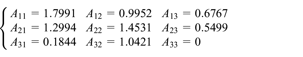
The state transition matrix P is calculated from the data in Table 4 using equations (15)–(17)

{\begin{matrix} A_{11} = 1.7991 A_{12} = 0.9952 A_{13} = 0.6767 \\ A_{21} = 1.2994 A_{22} = 1.4531 A_{23} = 0.5499 \\ A_{31} = 0.1844 A_{32} = 1.0421 A_{33} = 0 \end{matrix}

{\begin{matrix} {A'}_{11} = 0.5183 {A'}_{12} = 0.2867 {A'}_{13} = 0.1950 \\ {A'}_{21} = 0.3935 {A'}_{22} = 0.4400 {A'}_{23} = 0.1665 \\ {A'}_{31} = 0.1504 {A'}_{32} = 0.8496 {A'}_{33} = 0 \end{matrix} = P = [\begin{matrix} 0.5183 0.2867 0.1950 \\ 0.3935 0.4400 0.1665 \\ 0.1504 0.8496 0 \end{matrix}]

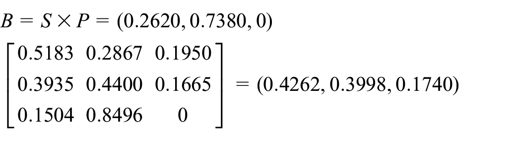
Given the fuzzy vector $S = (0.2620, 0.7380, 0)$ of the ninth group of data, the relative error data of the next state fuzzy transfer vector B can be obtained by combining S with the Markov state transition probability matrix P

\begin{matrix} B = S \times P = (0.2620, 0.7380, 0) \\ [\begin{matrix} 0.5183 0.2867 0.1950 \\ 0.3935 0.4400 0.1665 \\ 0.1504 0.8496 0 \end{matrix}] = (0.4262, 0.3998, 0.1740) \end{matrix}

According to equation (20), the relative error’s fuzzy correction $σ$ is obtained by multiplying the fuzzy vector B with the intermediate values of the error’s fuzzy state. The intermediate values of the fuzzy state $s_{1}, s_{2}, and s_{3}$ are −0.0431, 0.0358, and 0.1152, respectively

\begin{matrix} σ = (0.4262, 0.3998, 0.1740) \\ \times {(- 0.0437, 0.0358, 0.1152)}^{T} = 0.0157 \end{matrix}

Using $σ$ , the predicted value of 1.5557 in the 10th group in Table 3 is corrected by the fuzzy error, and the final predicted data are obtained as follows

{\hat{x}}^{(0)}^{*} (10) = \frac{{\hat{x}}^{(0)} (10)}{1 + σ} = \frac{1.5557}{1 + 0.0157} = 1.5317

PGFM (1,1) analysis example

The measured value of the 10th group measured in the experiment is 1.5239. With the traditional GM (1,1), the data of the 10th group were predicted to be 1.5621 with a relative error of 2.51%. With the PGM (1,1) model, the data of the 10th group were predicted to be 1.555, with a relative error of 2.09%. Finally, by combining PGM (1,1) with PGFM (1,1), the state of the 10th group of data was predicted to be 1.5317 with a relative error of 0.51%. It can be seen from the fitting effect and prediction accuracy of the same group of data shown in Figures 6 and 7 that with the gradual improvement of the traditional GM, the working accuracy of the newly formed composite model PGFM (1,1) is significantly higher and is closer to the engineering test data accuracy.

Figure 6.

Data fitting effect of groups 8–10.

Figure 7.

Comparison of the 10th group of data errors.

Nevertheless, the proposed PGFM (1,1) also has disadvantages in the calculation process. As PGFM (1,1) involves many steps, the operation process is relatively complex. The combined model is composed of a GM (1,1) and a one-step Markov state transition matrix, so it can accurately predict only the next state value. Although the prediction accuracy is improved, its computational complexity is high, and its scalability is insufficient.

Discussion

In section “Empirical study,” GM (1,1) is modified to PGM (1,1), which, in turn, is modified to PGFM (1,1) to predict and analyze the RMS vibration data of the full cycle life of the same set of bearings. The results showed that with the gradual improvement of the prediction method, the prediction accuracy of the 10th group of data as the validity test of the prediction model is gradually improved. Accordingly, it is proved that the proposed model is more suitable for the prediction of characteristic quantities of bearing vibration signals and can provide a powerful database for the accurate calculation of bearing residual life based on the WPHM.

GM (1,1) is less computationally expensive, and its predicted data can reach the basic standard. Therefore, it is suitable for the prediction of components’ characteristic quantities with low accuracy requirements. Compared with GM (1,1), PGM (1,1) increases the parameter correction step of the PSO algorithm, improves the prediction accuracy, and can meet the requirements of more engineering applications. PGFM (1,1) model is complex, and its prediction accuracy is higher than that of GM (1,1) and PGM (1,1). Therefore, this model is more suitable for predicting characteristic quantities of engineering structural components with high precision requirements. In general, with the modification of GM (1,1) to PGM (1,1) and then to PGFM (1,1), the accuracy, effectiveness, reliability, and applicability of the model become higher, but its complexity increases, as shown in Figure 8.

Figure 8.

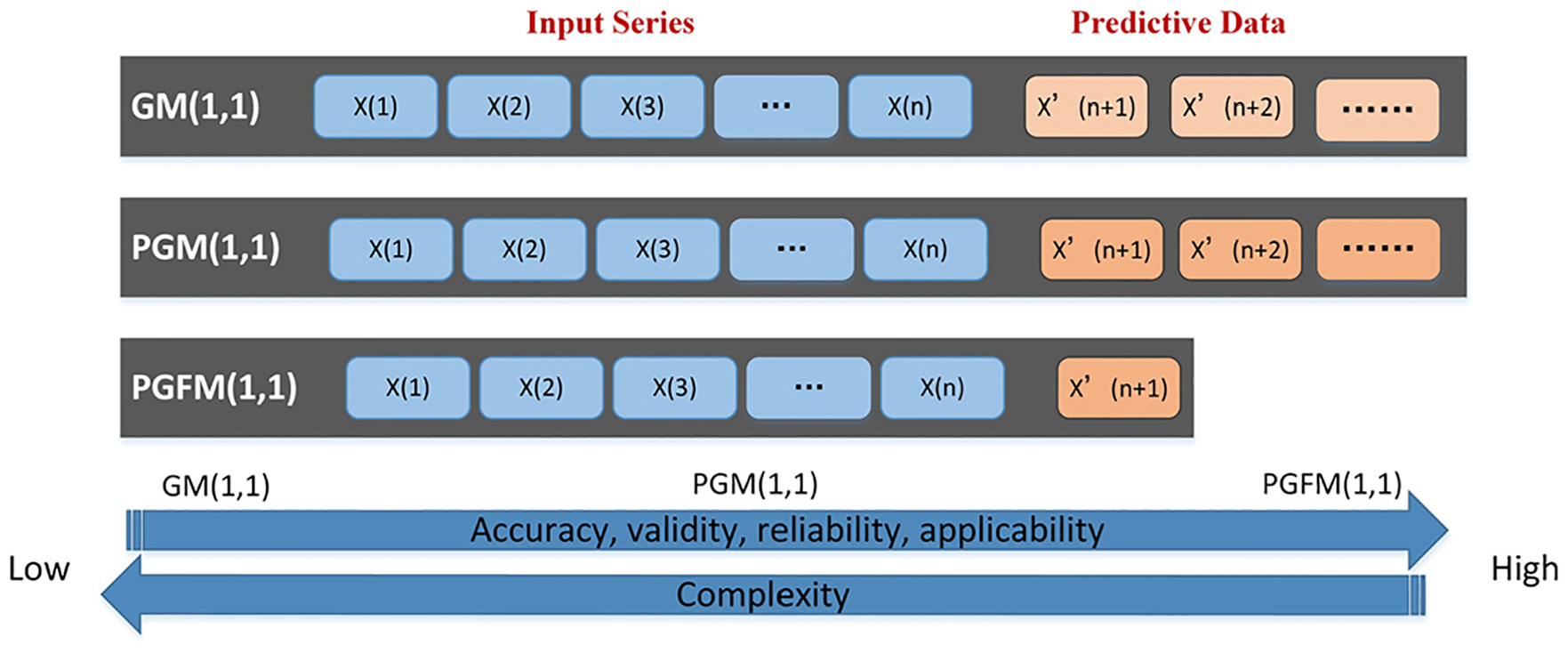
Diagram of the prediction models’ characteristics.

Considering the disadvantages of PGFM (1,1) and the advantages of PGM (1,1), we proposed a combination of the two models. First, PGM (1,1) can be used to predict the parameters that can represent the remaining lifetime components before the component fails. Then, the same parameters can be predicted with PGFM (1,1) for confirmation. The latest collected state data can be predicted by PGFM (1,1) to obtain more realistic prediction results.

Conclusion

Effective prediction methods are important to determine the running state of bearing equipment and formulate effective maintenance strategies. Although GM (1,1) is simple because it relies on a small amount of data for prediction, its prediction accuracy remains unsatisfactory. In this study, we analyzed the shortcomings of the original GM (1,1) in the prediction of parameters that can represent the state of bearings of marine propulsion shafting. Based on the traditional gray theory and combining the advantages of PSO, fuzzy mathematical theory, and Markov models, a new combined prediction model named PGFM (1,1) was proposed.

This proposed model has the following advantages: (1) it can be used to explore the internal law of time series and state transition sequence data and predict the future state; (2) it has a higher ability to predict the RMS vibration characteristics of bearings, which can guide maintainers and provide information on the future running state of the bearing; and (3) although PGFM (1,1) involves many theories, its operation is easy to understand and convenient for the compilation of specific programs; therefore, it can be easily applied to practical problems in many engineering fields.

The limitation of PGFM (1,1) is its applicability. (1) If the input data are not regular, the prediction accuracy can be poor. (2) Because PGFM (1,1) is a one-step Markov matrix established with a small amount of data, it is unable to predict the subsequent multi-set of data. However, PGM (1,1) can be used to predict multiple sets of dat. (3) Furthermore, the model is suitable for the prediction of one-dimensional time series, but not for multivariate or high-latitude data.

In future research, other theories can be considered for the modification of GM (1,1) to simplify the operation steps and improve the multi-step prediction ability.

Footnotes

Handling Editor: James Baldwin

Declaration of conflicting interests

The author(s) declared no potential conflicts of interest with respect to the research, authorship, and/or publication of this article.

Funding

The author(s) disclosed receipt of the following financial support for the research, authorship, and/or publication of this article: This research was supported by Zhejiang Provincial Natural Science Foundation of China under Grant no. LY20E090002 and Zhoushan City Science and Technology Planned Project under Grant no. 2018C21018.

ORCID iD

Yu Sun

References

Liu

. Research on the forecast method of rolling bearing life based on WPHM. Dalian, China: Dalian University of Technology, 2014.

Liao

Zhao

Guo

. Predicting remaining useful life of an individual unit using proportional hazards model and logistic regression model. In: RAMS ’06: annual reliability and maintainability symposium, Newport Beach, CA, 23–26 January 2006. New York: IEEE.

Deng

. Grey system overview. World Sci 1983; 7: 1–5.

Zhao

Guo

. An optimized grey model for annual power load forecasting. Energy 2016; 107: 272–286.

Zeng

, et al. Application of the novel fractional grey model FAGMO(1,1, k) to predict China’s nuclear energy consumption. Energy 2018; 165: 223–234.

Wei-Jun

Ming-Ye

. Algorithm to predict idle period based on grey model for dynamic power management. J Beijing Instit Technol 2005; 25: 963–966.

Liu

. Application of a novel time-delayed polynomial grey model to predict the natural gas consumption in China. J Comput Appl Math 2017; 324: 17–24.

Ming

Fan

Xie

, et al. A modified grey Verhulst model method to predict ultraviolet protection performance of aging B.mori silk fabric. Fiber Polym 2013; 14: 1179–1183.

Ning

Ding

Gong

, et al. Forecasting Chinese greenhouse gas emissions from energy consumption using a novel grey rolling model. Energy 2019; 175: 218–227.

10.

Han

. The non-equidistant new information MGRM(1,n) based on a step optimum constructing new information background value and accumulated generating operation of reciprocal number. J Xiangtan Univ 2016; 38: 10–14.

11.

Cun-Bin

Wang

. A new grey forecasting model based on BP neural network and Markov chain. J Cent South Univ 2007; 14(5): 713–718.

12.

Xie

Yuan

Yang

. Forecasting China’s energy demand and self-sufficiency rate by grey forecasting model and Markov model. Int J Electr Power Energy Syst 2015; 66: 1–8.

13.

Shen

. Grey-related least squares support vector machine optimization model and its application in predicting natural gas consumption demand. J Comput Appl Math 2018; 338: 212–220.

14.

Liu

Zhai

, et al. The improved grey model based on particle swarm optimization algorithm for time series prediction. Eng Appl Artif Intell 2016; 55: 285–291.

15.

Zimmermann

. Fuzzy set theory—and its applications. Berlin: Springer, 1985.

16.

Bon

Isah

. Hidden Markov model and forward-backward algorithm in crude oil price forecasting. IOP Conf Ser Mater Sci Eng 2016; 160: 012067.

17.

Guérin

Leiva-Leon

. Model averaging in Markov-switching models: predicting national recessions with regional data. Econ Lett 2017; 157: 45–49.

18.

Peng

Sun

Chen

, et al. Novel algorithm of light rail passenger trajectory prediction based on Markov chain. J Univ Electron Sci Technol Chin 2018; 47: 720–725.

19.

Nel

Mearns

Jordaan

. Trajectory analysis of informal Sand Forest harvesting using Markov chain, within Maputaland, Northern KwaZulu-Natal. Ecol Inform 2017; 42: 121–128.

20.

Yin

Yang

, et al. A Markov-based model for predicting the development trend of soil microbial communities in saline-alkali land in Wudi County. Concur Comput Pr Exp 2019; 31: e4754.

21.

. The research of Markov model forecasting method and application. Hefei, China: Anhui University, 2011.

22.

Liu

Wang

Zhang

. Grey systems: theory and application. Grey Syst Theor Appl 2011; 4883: 44–45.

23.

Lynn

Suganthan

. Ensemble particle swarm optimizer. Appl Soft Comput 2017; 55: 533–548.

24.

Korobkin

Kurklinskaya

Astachova

, et al. Application of the fuzzy logic theory in the problem prediction values of the technical coefficient. J Phys Conf Ser 2019; 1202: 012010.

25.

Yong

. Grey-Markov forecasting model and its application. Syst Eng Theory Pr 1992; 9: 59–63.

26.

Gang

. Grey-Markov model for forecasting road accidents. J Guangdong Commun Polytech 2006; 2006: 35–37.

27.

Chang

Sun

. Initial condition’s optimization on GM (1,1). In: Proceedings of 2011 IEEE international conference on grey systems and intelligent services, Nanjing, China, 15–18 September 2011. New York: IEEE.

28.

Jong

Liu

. Grey power models based on optimization of initial condition and model parameters. Grey Syst Theory Appl 2014; 4(2): 370–382.

29.

Haibing

Jia

Leikai

, et al. Analysis of settlement predicting effect of metabolic grey model under different initial condition. Site Invest Sci Technol 2016; 2: 48–51.

30.

Yang

. Research on multi-factor grey prediction and Markov chain fuzzy correction model of sales volume. Ind Eng Manag 2014; 19: 90–93+98.

Prediction and analysis of bearing vibration signal with a novel gray combination model

Abstract

Keywords

Introduction

Methodology

Standard GM (1,1) model

PSO

Fuzzy mathematical theory

Markov

PGFM (1,1) combined model

Empirical study

GM (1,1) analysis

PGM (1,1) calculation and analysis

PGM (1,1) calculation

PGM (1,1) analysis example

PGFM (1,1) calculation and analysis

PGFM (1,1) calculation

PGFM (1,1) analysis example

Discussion

Conclusion

Footnotes

Declaration of conflicting interests

Funding

ORCID iD

References