Sage Journals: Discover world-class research

Abstract

In the present research work, a finite element model of the electro-resistance welding pipe forming process chain is developed using the ABAQUS/Explicit software. The forming process, which is composed of 22 tandem roll stations, has been fully modeled in the developed finite element simulation. In order to account for the Bauschinger effect on the pipe material properties as a consequence of the loading and the unloading during the process, a non-linear kinematic hardening model has been utilized in all the proposed finite element simulation models. The constants for the non-linear kinematic hardening model were estimated by means of cyclic experiments on the K55 steel pipe material. In order to properly simulate the electric arc welding (electro-resistance welding) operation, the ABAQUS welding interface has been utilized to account for the joining between the two edges of the formed pipe as well as to assess the influence of the welding-induced temperature field on the residual stresses on the pipe material. The sizing operation, which is the final station of the electro-resistance welding process, has been also accounted in the developed finite element method model and is composed of six tandem rolls. To export and import the results between two different modules, a mapping strategy has been utilized and allowed exporting the element results, in terms of stress, strain, and temperature, and importing them into the following simulation module. Finally, in order to estimate the influence of each process station on the yield strength of the material, a finite element simple tension test simulation has been implemented in ABAQUS/Static, mapping the results of each station on the tensile specimen. This mapping operation allowed to estimate the yield stress of the material after each of the three process stations, a consequence of the residual stresses present in the material, and has been carried out on eight circumferential locations around the pipe, evenly spaced with a 22.5° angle. The model has been validated by comparing the geometrical results, in terms of average pipe diameter and thickness, obtained from the finite element model with those of the relevant industrial production, showing deviations equal to 1.25% and 1.35% (forming) and 1.29% and 1.43% (sizing), respectively, proving the reliability of the proposed process chain analysis simulation. The results will show how the process-induced residual stresses arising on the pipe material make the material yield strength to vary from station to station as well as having different values along the circumferential direction of the pipe.

Keywords

Electro-resistance welding process non-linear kinematic hardening model pipe forming process chain analysis forming simulation welding simulation

Introduction

The ERW (electro-resistance welding) process used in the production of pipes is a well-established industrial manufacturing technology in which a flat metal strip is progressively deformed by sets of rotating rolls arranged in tandem.¹ Pipes produced by the ERW process have diameters and thicknesses ranging from 30 to 600 mm and from 3 to 15 mm, respectively, and are employed, as well as pipelines and structures, in the automotive industry.

The ERW process (Figure 1) is normally composed of three main operations: (1) a forming station, where the metal sheet is deformed from the plane strip to the pipe shape; (2) a welding station, in which the two edges of the strip are welded together; and (3) a sizing station, where the welded pipe passes through several rolls and is then sized into the final dimensions.

Figure 1.

The ERW pipe forming process.

In the literature, different authors have analyzed the forming station of the ERW pipe forming process, both from the analytical and finite element method (FEM) points of view. Han et al.¹ utilized a B-spline finite strip method to describe the evolution of longitudinal strains, opening value, and springback. Their results are shown to be in good agreement with the relevant experiment and proved that, in the ERW pipe forming process, the springback effect is small and, therefore, negligible. Walker and Pick^2,3 developed an analytical model for the description of the deformation path during the forming process, analyzing the influence of the process parameters on the quality of the final product. Jiang et al.⁴ studied the ERW process from an FEM point of view, allowing to identify the so-called “no-bending area” in the strip as well as important parameters, such as the longitudinal strain, the opening distance, and the geometry of the deformed strip; the validation has been carried out by comparing the results of the finite element (FE) model with those of industrial experiments, showing the reliability of their approach. Recently, Kasaei et al.⁵ utilized the MSC Marc/Mentat software to simulate the cage roll forming process of ERW pipes and developed an edge-buckling criterion, concluding that the edge buckling is unavoidable if the initially selected width is bigger than a specific limit.

Concerning the estimation of the yield strength after the pipe forming process, two recent contributions are available. Lee et al.⁶ studied the influence of the variation in the yield strength of the material due to the forming process, considering its different values along the circumferential direction of the pipe. In addition, Jo et al.⁷ analyzed the reduction in the yield strength in the pipe, in comparison to that of the original strip, from the microstructure point of view. The conclusion of their research showed that, in order to prevent a significant yield strength reduction after the forming process, low-temperature transformation microstructures, coarse grain size, and high pipe thickness/diameters should be achieved.

Concerning the electro arc welding (ERW) operation, the second stage in the considered pipe manufacturing process, a few contributions related to this topic are available in the literature, as follows. Wen et al.⁸ studied both the heat transfer and the heat-affected zones during the welding process, defining an optimization algorithm to reduce both geometrical distortions and residual stresses. Sattari-Far and Javadi⁹ developed an FE model to study the influence of the welding sequence on the welding-induced distortion in the pipe, analyzing nine different approaches of pipe front-face welding and concluding that the choice of a proper welding strategy can reduce the distortion in the final product. Deng et al.¹⁰ studied the residual stresses in the front-to-end face welded pipes by means of FE simulations, determining the welding temperature field during the welding operation and predicting the residual stress after the process. In another work, Deng and Murakawa¹¹ also developed a mixed two- and three-dimensional (2D and 3D) FE approach for the residual stresses and temperature field estimation in the multi-pass welding operations for stainless steel pipes, proving good agreement with the experimental results. Furthermore, Akbari and Sattari-Far¹² studied the welding-induced heat influence on the residual stress after the process for butt welds of pipes realized with dissimilar materials by means of FE simulations.

Although several authors have analyzed the forming part of the ERW pipe manufacturing process, only a few studied the welding operation. In addition to that, no contributions seem to deal with the whole process chain with the aim of determining the combined effect of forming, welding, and sizing operations on the yield strength of the material.

In the forming process, since the strip is subjected to continuous tensile and compression stresses, the yield stress of the material varies several times due to the Bauschinger effect. In addition, as a consequence of the temperature difference between the welding area and those nearby, the ERW operation creates additional residual stresses, while partially releasing those from the forming process. Since both forming and welding operations result in non-uniform residual stress distribution on the pipe, the yield stress is not uniform along the circumferential direction and, as it will be shown in the result section, both results differ from the original yield stress of the material.

For this reason, a precise estimation of the circumferential distribution of the yield strength of the pipe, after the whole process (forming, welding, and sizing), is of critical importance for the industry in order to provide a precise estimation to the end users. In the real production process, a direct measurement of the yield strength of the pipe is not feasible since the cutting operation needed to realize the specimen would partially or completely release the residual stress, making the measurement to be imprecise or even meaningless. Therefore, a reasonable way to estimate the different amounts of residual stresses along the circumferential direction is to develop an FE process model including the whole process chain, from the beginning of the forming to the end of the sizing.

In the research presented in this article, three different FE models have been developed and are relevant for the (1) forming, (2) welding, and (3) sizing processes. The forming FE model is composed of 20 roll passes carried out by identical twin rolls, with the exception of the last station, which is composed of 4 rolls. The material fed to the rolling mill has an initial width and thickness of 680 and 8.84 mm, respectively, and, at the end of the forming, the pipe reaches a diameter equal to 691 mm. After the forming process, the results are mapped into the ABAQUS welding interface (AWI), where the temperature field resulting from the ERW is first calculated. In addition to that, in the welding FE simulation, the gap between the two edges of the pipe is filled by layers of elements, allowing to simulate the result of the ERW process. After the welding operation is completed, the results are mapped into the sizing FE model, composed of six tandem rolls. In addition to that, in order to understand the influence of the sizing ratio on the residual stress, three different study cases, considering a sizing ratio of 0.2%, 1.0%, and 1.5%, have been analyzed and the results are detailed in the article.

The FE models have been modeled with hexahedron type C3D8R elements, and considering a Coulomb friction coefficient equal to 0.2 (only for forming and sizing) and in order to limit the computational burden, only a portion of the whole metal strip, 500 mm long, has been modeled with fine mesh, whereas the rest, 1500 mm long, has been modeled with a coarser mesh.

After each station, the results belonging to the elements of the fine mesh section are exported and mapped into a simple tension test specimen shape. The data are saved at each 22.5° interval along the circumferential direction and for a length of 165 mm, allowing to determine the different material properties of the pipe for different positions around the diameter. As it will be shown in the result section, the yield strength of the material is influenced by the three different process stations, and this results in a range of variation for the yield strength from 50 to 100 MPa, in comparison to the original one of the metal strip.

Since, for the above-mentioned reasons, no validation on the basis of the residual stress is feasible, the validation of the proposed FE simulation models has been carried out by comparing the dimensions of the cross-section of the pipe (diameter and thickness), resulting from the real production, with those of the FE models. The comparison is operated after the forming and after the sizing stations, and the average and maximum deviations, relevant for pipe diameter and pipe thickness, have been calculated in 1.25% and 1.35% (forming) and 1.29% and 1.43% (sizing), respectively.

The proposed mapping operation allows avoiding any loss of information and grants a proper and precise estimation of the yield strength of the material for each one of the tested circumferential positions of the pipe and after each station of the process. The variation of the yield strength is directly linked to the amount of residual stress in the pipe, properly estimated by the developed FE models.

The full process chain analysis of the ERW pipe forming process proposed in this article allows the determination of important pipe geometrical data (diameter, thickness, and circularity) as well as the yield strength distribution in the final product, giving precise information to be used as a reference for the pipe utilizers. In addition to that, if process modifications are meant to be tested, the influence of the variation of the process parameters on the yield strength of the pipe can also be determined by means of the developed FE models, allowing to limit the amount of the required production tests, which are expensive and high-time consuming procedures.

Non-linear isotropic/kinematic hardening model

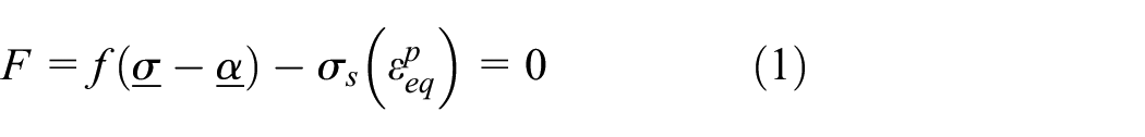
In order to take into account the Bauschinger effect caused by the continuous application of tension and compression loads during the process, the non-linear kinematic hardening (NLKH) formulation is utilized in the FE model presented in this article. The general formulation for the yielding surface $(F)$ is defined by equation (1), which is composed of two terms, a kinematic one and an isotropic one. The combination of these two hardening effects make the yield surface both to translate, according to the backstress tensor $\underline{α}$ , and to expand in the stress space, as a consequence of the variation of the plastic strain $ε_{eq}^{p}$ , hence the yield stress $σ_{s}$ . This combined effect is shown in Figure 2

F = f (\underline{σ} - \underline{α}) - σ_{s} (ε_{eq}^{p}) = 0

(1)

Figure 2.

Yield surface change in the principal space due to plastic deformation.

Being that the yield surface is the combination of two different types of hardenings, isotropic one and kinematic one, the two effects can be separately analyzed. Considering the kinematic hardening part, the equivalent stress, function of the stress tensor and of the backstress tensor, is defined as in equation (2) where the symbol × indicates the inner product between tensors. The NLKH formulation was first introduced by Armstrong and Frederick,^13,14 equation (3), and afterward modified by Chaboche,¹⁵ who widened its range of application, by considering a superposition of a number of same models equal to the size of the backstress tensor.

The formulation reported in equation (4), due to Fu et al.,¹⁶ is a different representation of the original one due to Chaboche,¹⁵ and it is particularly useful for the implementation of the NLKH model in the FE program ABAQUS.¹⁷ Thus, in this research work, the model of equation (4) has been utilized for the development of the FE model. The summation of the single component of the backstress tensor is performed, as shown in equation (5), where n is the size of the backstress tensor (number of components). The size of the backstress tensor is normally determined in order to have an accurate fitting of the experimental results. Finally, the isotropic part of the hardening is expressed by means of Voce’s model, as shown in equation (6)

f (\underline{σ} - \underline{α}) = \sqrt{\frac{3}{2} ({\underline{σ}}^{dev} - {\underline{α}}^{dev}) \times ({\underline{σ}}^{dev} - {\underline{α}}^{dev})}

(2)

d \underline{α} = \frac{C}{σ_{s}} (\underline{σ} - \underline{α}) d ε_{eq}^{p} - γ \underline{α} d ε_{eq}^{p}

(3)

d {\underline{α}}_{i} = \frac{C_{i}}{σ_{s}} (\underline{σ} - \underline{α}) d ε_{eq}^{p} - γ_{i} {\underline{α}}_{i} d ε_{eq}^{p}

(4)

\underline{α} = \sum_{i = 1}^{n} {\underline{α}}_{i}

(5)

σ_{s} (ε^{p}) = {σ_{s}}^{0} + A (1 - e^{b \cdot ε_{eq}^{p}})

(6)

In order to characterize both the kinematic and the isotropic hardening behaviors, the material constants ${σ_{s}}^{0}$ , A, and b, for the Voce model equation (6), and $C_{i}$ and $γ_{i}$ (as many as the size of the backstress tensor), for the modified-Choboche model of equation (4), must be derived from the best fitting of the cyclic loading test results. In the following paragraph, the material characterization experiments are presented, and the relevant kinematic and isotropic hardening model constants are derived.

Characterization of K55 steel mechanical properties

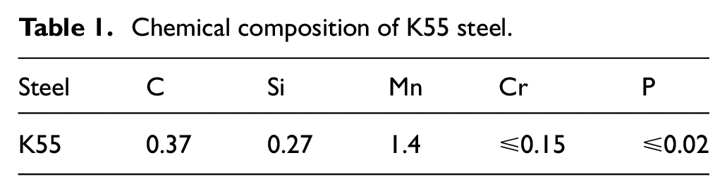
In order to determine the material constants for the utilized NLKH model, as described in the previous section of the article, tensile experiments have been carried out and the details are reported in this section. The pipe material considered in this research is the K55 steel, largely utilized for the production of pipes in the ERW process, and its chemical composition is reported in Table 1. In order to determine the material properties to be used in the FE model, static and low cyclic loading tests have been conducted on specimens made of the same material of the pipe. The dimensions of the specimen utilized in both static and cyclic loading tests are summarized in Figure 3(a), whereas the test machine with the installed specimen and strain gauge is shown in Figure 3(b).

Table 1.

Chemical composition of K55 steel.

Steel	C	Si	Mn	Cr	P
K55	0.37	0.27	1.4	≤0.15	≤0.02

Figure 3.

(a) Test specimen (ASTM E8 standard) and (b) cyclic loading test.

In the experiment, the tensile speed of 1 mm/min has been utilized in both static and cyclic loading tests. In the static test, the failure displacement has been measured in 2.5 mm; thus, in the cyclic test, a stroke amplitude equal to 2.45 mm has been utilized, allowing to reach the specimen failure after one cycle, as reported in Figure 4.

Figure 4.

Static and cyclic true stress–strain curves for the K55 steel specimen.

In the ERW welding process, no additional material is applied in the welding zone and the joining is operated by welding together the edges of the strip. The material is molten by the electric flow in the pipe and the application mechanical pressure makes the material to squeeze in the gap between the two edges of the strip, creating the weld joint. The additional data required for the proper setup of the welding simulation have been derived from the MATILDA^® (Material Information Link and Database Service) archive, an online material database with referred material data. In Table 2, the specific heat capacity and the conductivity, for increasing temperature, are reported.

Table 2.

K55 material data for the welding operation.

Temperature (°C)	Specific heat capacity (J/g°C)	Conductivity (J/mm°Cs)
0	0.462	0.0146
100	0.496	0.0151
200	0.512	0.0161
300	0.525	0.0179
400	0.540	0.0180
600	0.577	0.0208
800	0.604	0.0239
1200	0.676	0.0322
1300	0.692	0.0337
1500	0.700	0.1200

ERW FE process chain analysis

Calibration of K55 steel material properties

The material properties of the K55 steel have been calibrated in the FE simulation by considering a size 3 for the backstress tensor. The FE simulation has been implemented in ABAQUS/Standard conspiring the same geometry and the same testing conditions summarized in the “Characterization of K55 steel mechanical properties” section of the article. The parameters for the NLKH model, equation (4), and for the Voce flow stress model, equation (6), are reported in Table 3, along with the Young’s modulus of the material.

Table 3.

K55 steel properties and NLKH model constants.

E (Gpa)	$σ_{s}^{0}$ (Mpa)	A	b	$C_{1}$	$γ_{1}$	$C_{2}$	$γ_{2}$	$C_{3}$	$γ_{3}$
207	390	160	8	9650	95	100	25	20	35

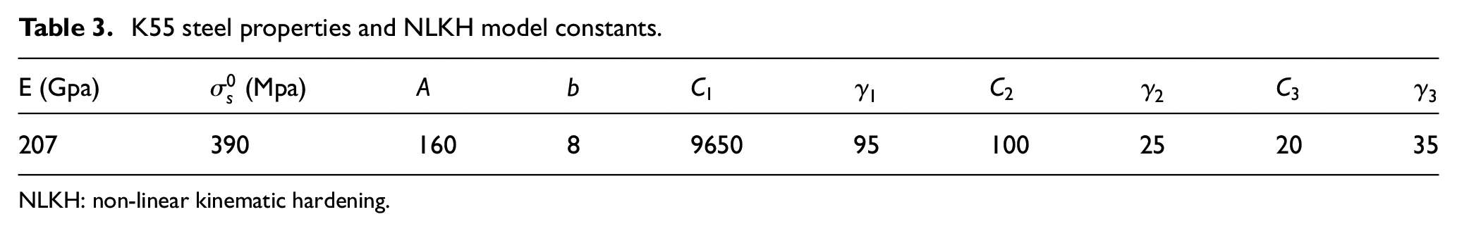
NLKH: non-linear kinematic hardening.

The reasoning behind the utilization of a size 3 for the backstress tensor is given by the need for minimizing the difference between experimental and FE results and, at the same time, limiting the computational time. For these reasons, FE simulations have been implemented considering a backstress tensor size equal to 2, 3, and 4, identifying in the size 3 the best compromise between accuracy and computation burden. The difference between the area beneath the experimental curve and the model-fitted one has been calculated in 9.12%, showing the reliability of the choice of the size of the backstress tensor. The comparison between experimental and FEM true stress–strain curves for the cyclic loading, previously shown in Figure 4, is reported in Figure 5. These material properties, relevant for the K55 steel, have been utilized in the process chain FE simulation described in the following paragraphs.

Figure 5.

Static and cyclic true stress–strain curves for the K55 steel specimen.

FE simulation models’ interaction overview

In order to properly estimate the residual stresses in the pipe after each station of the process, as well as its influence on the yield strength of the pipe material, all the three main stations of the ERW pipe manufacturing process have been included in the developed FEM model. Since the welding simulation requires a different ABAQUS module, it is necessary to separate each station, resulting in three different FE models: one for the forming, one for the welding, and finally one for the sizing operation. As it will be shown in this section of the article, in order to export the results from one module and input them into the following one, a data mapping strategy has been developed, allowing to save the data of position, stress, strain, temperature, and so on, of each elements of a fine mesh portion of the pipe, to be inputted in the input file of the following analysis. Moreover, after each stage, the results of the fine mesh section of the pipe are exported and mapped in the simple tension test simulation, where the yield strength of the material is calculated. Thanks to the utilization of the NLKH model, the local residual stresses around the circumference of the pipe are accounted for, allowing to estimate their influence on the yield strength of the material. The FE process chain analysis, including the testing stages, is shown in Figure 6.

Figure 6.

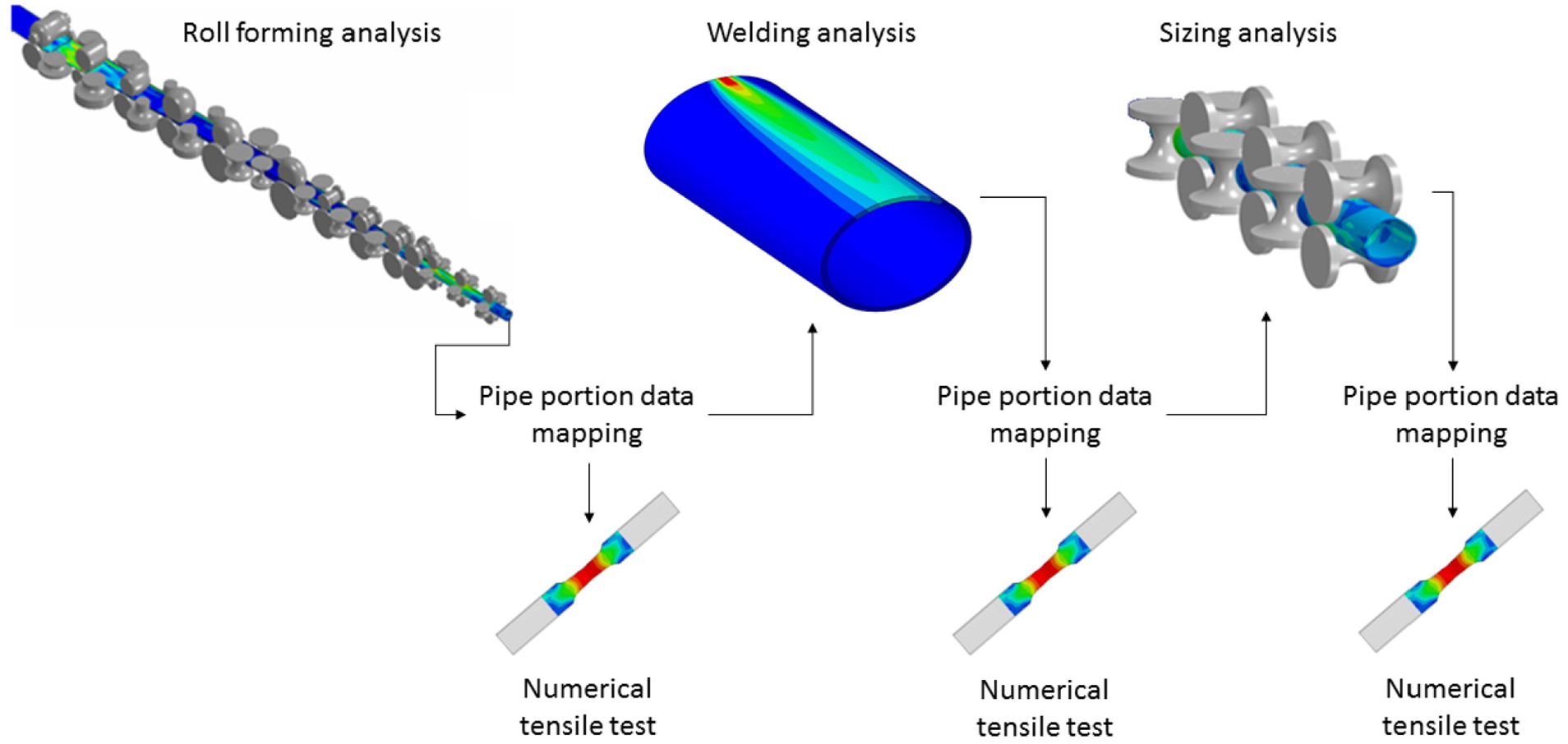
Process chain analysis and intermediate mapping/testing strategy.

In the following four sections of the article, the simulation of the three process stations, as well as that for the material testing (tensile), is explained in detail, showing also an introductory perspective of the results of each stage.

Roll forming analysis

The first part of the FE model focuses on the forming process, composed of 20 tandem rolls, where the initial metal strip is progressively bent in order to reach the pipe shape. The simulation is implemented in ABAQUS/Explicit, and all the relevant information about simulation settings and boundary conditions are described in this paragraph. The initial steel strip is directly designed inside the ABAQUS interface, with the following dimensions: 13,170 mm length, 670 mm width, and 8.83 mm thickness. In order to reduce the computational time, only a 500-mm portion of the pipe is meshed with fine elements, whereas the remaining parts are modeled with coarser one. This strategy allows keeping the overall stiffness of the pipe while reducing the computational time. The flat metal strip and the initial two couples of rolls, at the beginning of the simulation, are shown in Figure 7, where the two different mesh zones are identified.

Figure 7.

Beginning of the forming simulation.

Both fine and coarse zones are meshed utilizing the C3D8R hexahedron elements, which allows calculating precise results while reducing the overall computational time, as demonstrated by Zou et al.¹⁸ for the roll forming process, Tajyar and Abrinia¹⁹ for the non-circular tube forming process, Cai et al.²⁰ for the roll forming process, and Yang et al.²¹ and Guo and Yang²² for the ring rolling process. The C3D8R is a general-purpose linear brick element, with reduced integration, in which the integration point is located at the center of the element volume. In the forming simulation, the fine mesh elements have the following dimensions: 2.25 mm width, 10.0 mm height, and 6.0 mm length, whereas the coarse mesh has the following dimensions: 4.5 mm width, 10.0 mm height, and 30 mm length, for a total of 72,000 elements.

The forming simulation is composed of 20 roll passes, where each roll has a rotational speed set to 4 rad/s and is modeled as analytical rigid. The friction is modeled by setting the Coulomb coefficient to 0.2, and the environment temperature is set to the room temperature of 20°C. The schematic representation and the FEM implementation of the whole forming process are shown in Figure 8.

Figure 8.

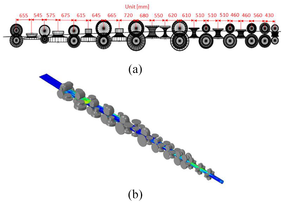
(a) Forming process schematic and dimensions, and (b) forming simulation.

At the end of the forming process, although the whole steel strip has been deformed by the sequence of all the rolls, the target results are those from the fine mesh section of the pipe. An example of the 3D representation of the fine mesh section of the pipe after the forming process, and of its cross-section, is shown in Figure 9. The details in Figure 9(b) show the zone where the welding operation will be done between the two extreme edges of the strip.

Figure 9.

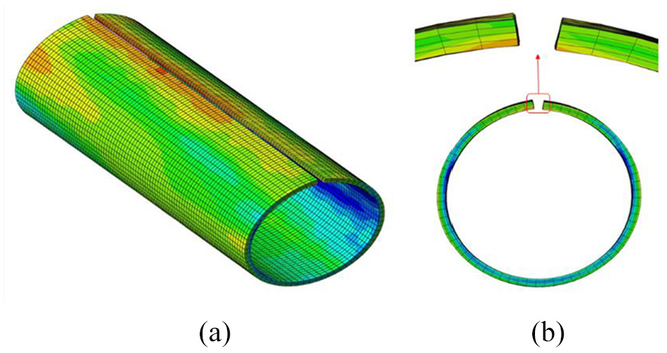
(a) Output of the forming simulation and (b) cross-section of the pipe after forming.

At this point, as shown in Figure 6, the results of the elements belonging to the fine mesh section of the pipe are exported and mapped into a simple tension test specimen shape, for the estimation of the yield strength of the material. The export and mapping operation is hereafter explained, whereas the simple test simulation is described in the “Sizing analysis” section since its FE model is the same for all the three intermediate steps.

The output of the forming simulation is exported as a list of mesh element coordinates and simulation results (stress, strain, temperature, etc.), to be inputted in the following welding module. A graphical example of the mapping operation is shown in Figure 10, where the original FEM result model is converted into a cloud of element nodes. The export of the results is carried out by an external algorithm, implemented in MS Excel, which allows extrapolating the selected sets of results for each element of the mesh and mapping them into the ABAQUS input file of the following simulation. This operation is carried out for the mapping from the forming to the welding, from the welding to the sizing, and also for the mapping after each one of the three process stations (forming, welding, and sizing) to the tensile test FE model, as previously summarized in Figure 6.

Figure 10.

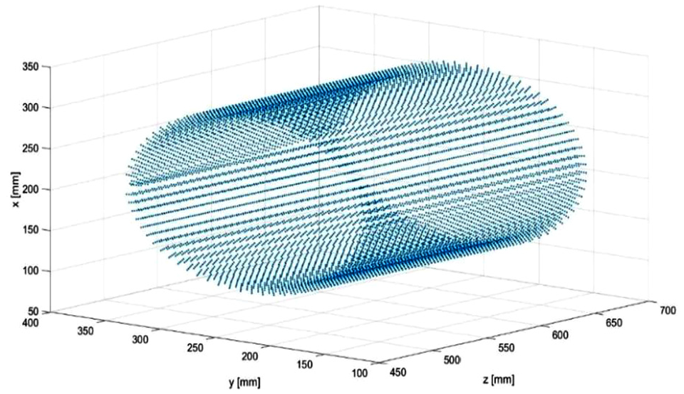
Mapping of the fine section node data (example of nodes cloud).

Since the mapping operation is a high time-consuming strategy, authors have chosen to export three different sections of the fine mesh portion of the pipe at the end of the forming simulation and to map them into the input file of the welding simulation. This approach is based on the assumption that each one of these three results will cover 1/3 of the total length of the fine mesh portion of the pipe (Figure 11). The comparison between the output results of the forming simulation and the input mapped data for the welding simulation is shown in the result section, where it will be shown that the adoption of this approach does not significantly alter the results but allows a considerable spare of time.

Figure 11.

Output of the forming simulation and mapping operation.

Welding analysis

The welding simulation is set up in the appropriate ABAQUS module where, following the data mapping operated from the previous simulation (forming), the ABAQUS input file is edited importing the data of the nodes those belong to the fine mesh portion of the pipe. In the first step of the welding simulation, the stress–strain state is the mapped one from the previous simulation, as schematically shown in Figure 11. As previously pointed out, the mapping operation allows transferring the data from the ABAQUS/Explicit module to AWI, and vice versa. In the welding simulation, the material parameters previously listed in Table 3 are utilized along with the additional process settings, shown in Table 4.

Table 4.

Additional process settings of welding simulation.

Parameter	Value
Welding speed	5 cm/s
Welding temperature	1450°C
Ambient temperature	20°C
Emissivity	0.4
Heat transfer coefficient	25 W/m² K

In the real ERW process, the material of the two edges of the strip is molten and, due to the applied pressure, the gap is filled, making the pipe to assume its final closed shape. In the developed FE model, the welding operation is simulated by the progressive addition of mesh elements in the gap between the two edges, as shown in Figure 12, where the dimensions of the added elements are reported. Although the addition of the element in the gap between the two edges of the pipe is slightly different from the original welding operation carried out in the ERW process, its influence on the final geometry of the pipe is almost negligible, as it will be shown in the “Results and discussion” section of the article.

Figure 12.

Mesh addition size in the welding simulation (dimensions in millimeters).

Finally, at the end of the welding, the results are exported and mapped into the sizing simulation, presented in the next paragraph, following the same procedure shown in Figure 10.

Sizing analysis

As previously operated for the export of the data from the forming simulation to the welding one, the same export/mapping procedure is applied to input the data in the sizing FE model. Also in the sizing simulation, composed of six tandem rolls, the C3D8R hexahedron element has been used to mesh the whole domain. In order not to directly start the simulation with the fine mesh section, and to properly consider the stiffness of the whole pipe, before the fine mesh part, a coarse mesh section of 1500 mm length, with the same diameter of the fine mesh portion, has been added. This addition is carried out by linking a 1500-mm coarse mesh portion of the pipe to the front of the fine mesh one, and this operation is carried out directly in the input file of the sizing FE model.

In the sizing station, all the rolls rotate at the same rotational speed of 4 rad/s, and they all share the same geometrical dimensions as schematically shown in Figure 13(a). In Figure 13(b), the FE implementation in ABAQUS/Explicit is also shown. Finally, the Coulomb friction is set to 0.2 as specified by the industrial partner, whereas the environment temperature is specified to be 20°C.

Figure 13.

(a) Sizing process schematic and dimensions, and (b) sizing FE simulation.

One of the key parameters for the pipe forming process is the sizing ratio, which stands for the ratio between the pipe diameter before and after this station of the process and can significantly influence the final yield stress of the material. For this reason, by utilizing the same model described in this paragraph, three different sizing ratios have been tested, and the influence of this variation on the yield stress of the material is presented in the “Results and discussion” section of the article.

At the end of the sizing station, also end of the whole ERW process, the results are exported and mapped on a simple tension test specimen for the FEM estimation of the yield strength of the material. In the following section, the mapping operation to realize the simple tension test specimen starting from the results of the three stations of the ERW process will be explained and the boundary and load condition, relevant for the model, will be detailed.

Simple tension analysis

In order to estimate the yield strength of the material after each station of the process, a simple tension test FE simulation has been implemented in ABAQUS/Static. The calibrated potion of the specimen has been modeled utilizing the C3D8R elements, with the following size: 2.0 mm width, 1.5 mm length, and 2.2 mm height, for a total of 384 elements. The remaining two portions of the specimen have been modeled utilizing the same element, with the following dimensions: 3.3 mm width, 3.0 mm length, and 2.3 mm height, for a total of 360 elements. Based on the data exports operated after each of the three process stations, nine different simple tension test specimens are realized along the longitudinal direction at different angular positions, starting from the 0° position (welding zone) to 180° position (opposite to the welding zone), for a total of 27 results for each complete process chain analysis. The dimensions of the specimen are those from the ASTM E8 Type 1 standard, reported in Figure 14. One side of the specimen has been fully blocked in all the directions, whereas on the other side, a 4-mm displacement has been applied. Moreover, in order to simulate the areas blocked by the gigs of the tensile machine, the two extremes of the specimen have been modeled as rigid and are represented by the gray zone on the two extremes of the specimen (Figure 14).

Figure 14.

ASTM E8 standard specimen.

For the mapping of the results of each forming station into the simple tension test specimen shape, the procedure explained hereafter is utilized. The pipe is subdivided into 22.5° sectors along the circumferential direction and a 165-mm long portion is identified, as shown in Figure 15(a). For each angular section, an upper area and a lower area are identified and, for each of them, the value of the stress and strain components along with the three directions, as well as the equivalent plastic strain PEEQ, is exported, averaged, and mapped into the simple tension test specimen.

Figure 15.

(a) Angular mapping subdivision of the pipe and (b) data mapping in the simple tension test specimen.

The data relevant for the upper section of the simple tension test specimen are the averaged ones of the upper section of the relevant pipe section, whereas the lower one comes from the lower part of the pipe section instead, as shown in Figure 15(b). Moreover, both pipe and simple tension test specimen have four elements along the thickness direction, allowing to map an average stress state for each of these four layers.

The described procedure allows creating a simple tension test specimen that includes the mapping data of two adjacent areas of the pipe, along the longitudinal direction, taking into account possible variation of the residual stress even inside the same specimen. Moreover, the one-to-one mapping along the thickness accounts for the intrinsic variation of the stress field between the outer and the inner diameters of the pipe due to different tension and compression process–induced stress states.

Results and discussion

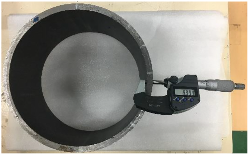
In order to validate the proposed FE model, since a direct verification based on the estimation of the yield strength of the pipe is not feasible, the geometrical results of the FEM simulation, in terms of thickness, average diameter, and circularity of the pipe, have been compared with those of the real production. To do so, both the thickness and the diameter of the pipe have been measured after forming and after the sizing stations, as shown in Figures 16 and 17, respectively. The results are reported in Table 5. The average diameter of the pipe has been calculated from the measurement of the circumference of the pipe, divided by π. For the calculation of the circularity, the diameter of the pipe has been measured each 60° around the pipe by means of a graduated scale.

Figure 16.

Pipe circumference measurement in real production (for the diameter calculation).

Figure 17.

Pipe thickness measurement in real production.

Table 5.

Comparison of pipe geometrical results between production and FEM measurements.

Dimension	Production measurement (mm)	FEM result measurement (mm)	% error
Diameter (after forming)	220.7 ± 1.0	219.94	1.25
Thickness (after forming)	8.96 ± 0.001	8.87	1.35
Diameter (after sizing, ratio 0.2)	217.6 ± 1.0	216.63	1.29
Thickness (after sizing, ratio 0.2)	9.03 ± 0.001	9.16	1.43
Circularity (after forming)	1.35	1.07	20.7
Circularity (after sizing, ratio 0.2)	0.53	0.46	13.2

FEM: finite element method.

The error intervals shown in Table 5 are due to the instrument, for the production measurements, and due to a circularity error detected during the measurement of the diameter from the FE simulation. In spite of these small differences, the agreement between the results of the FE model and those of the real production confirms the quality of the developed model in replicating the real process, since the error is limited to a maximum of 1.25% in the estimation of the diameter and to 1.43% for that of the thickness. In order to validate the mapping operation utilized to exchange the simulation results between different ABAQUS modules, the results of the von Mises equivalent stress at the end of the forming simulation and the step 0 (after mapping) at the beginning of the welding simulation are reported in Figure 18.

Figure 18.

The von Mises equivalent stress field at the (a) end of the forming and (b) beginning of the welding (after mapping).

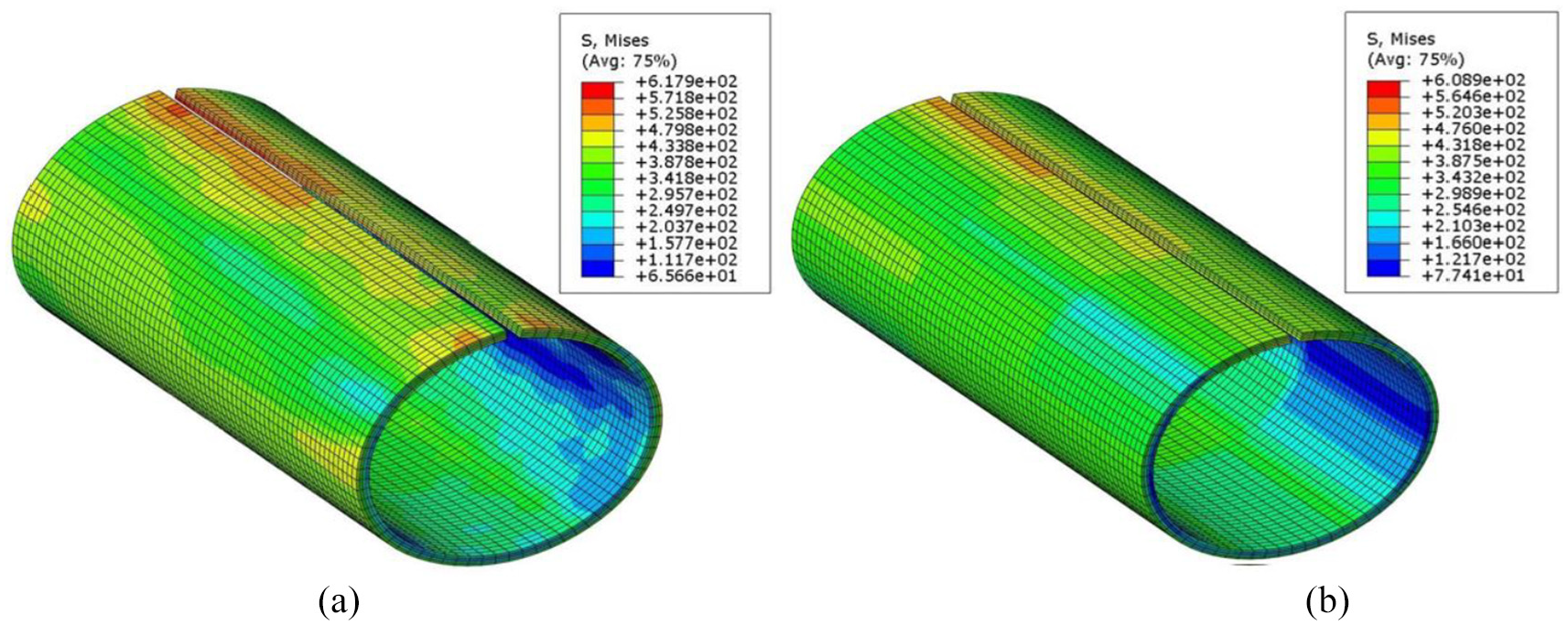
In the same way, the comparison between the results at the end of the welding simulation and those at the beginning of the sizing one (step 0), after mapping, is shown in Figure 19, same in terms of von Mises equivalent stress. The comparison of the results shown in both Figures 18 and 19 highlights a very good agreement between the stress fields before and after the mapping, proving the reliability of this strategy in exporting and importing data between different modules of the ABAQUS software. In addition to the results shown in Figures 18 and 19, the equivalent von Mises stress after the sizing process, for the fine mesh portion of the pipe, is shown in Figure 20 for the three different analyzed forming ratios.

Figure 19.

The von Mises equivalent stress field at the (a) end of the welding and (b) beginning of the sizing (after mapping).

Figure 20.

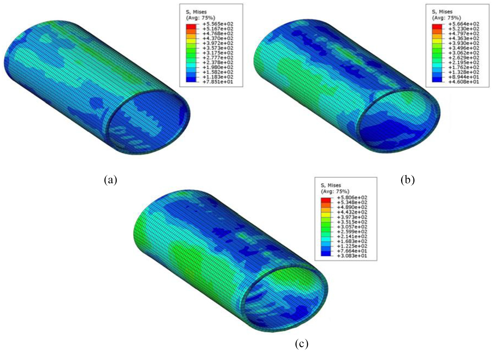
The von Mises equivalent stress after the sizing for (a) 0.2 sizing ratio, (b) 1.0 sizing ration, and (c) 1.5 sizing ratio.

In Figures 21 –23 instead, the results of the PEEQ (equivalent plastic strain) after each one of the stations of the process are presented, detailing the differences due to different sizing ratios. Finally, the temperature at the end of the welding operation is shown in Figure 24.

Figure 21.

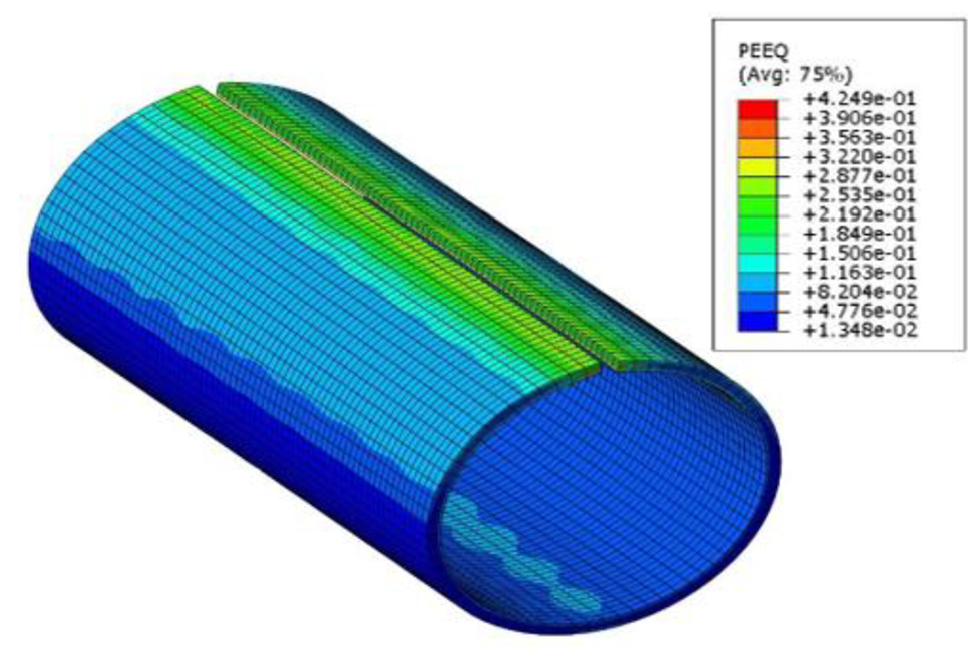
Equivalent plastic strain (PEEQ) after the forming station.

Figure 22.

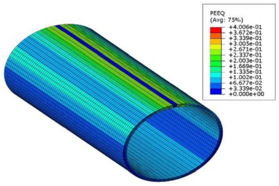
Equivalent plastic strain (PEEQ) after the welding station.

Figure 23.

Equivalent plastic strain (PEEQ) after the sizing for (a) 0.2 sizing ratio, (b) 1.0 sizing ratio, and (c) 1.5 sizing ratio.

Figure 24.

Temperature field at the end of the welding simulation.

Concerning the FE simple tension tests for each one of the nine angular positions of the pipe, the results are presented in Figure 25, after the forming station; in Figure 26, after the welding one; and in Figure 27, after the sizing process. In Figure 27, three different curves relevant for the three tested sizing ratios (0.2, 1.0, and 1.5) allow seeing the influence of this parameter on the yield strength of the material.

Figure 25.

Yield strength in the pipe for different angular positions after the roll forming process.

Figure 26.

Yield strength in the pipe for different angular positions after the welding process.

Figure 27.

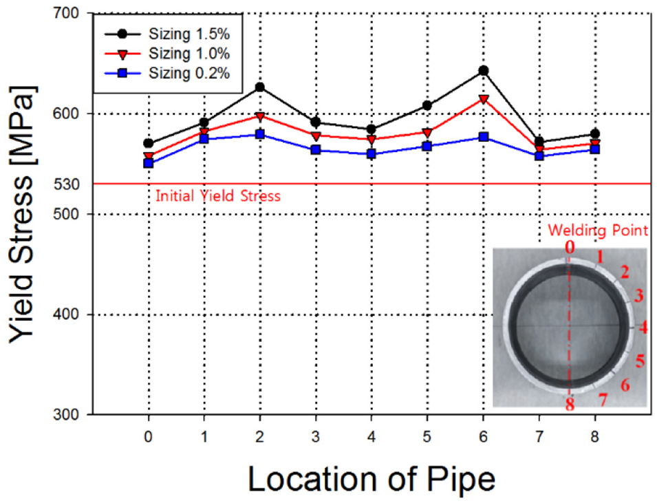
Yield strength in the pipe for different angular positions after the sizing process and for different sizing ratios.

The results of Figures 25 –27 show the angular position-dependent yield strength of the material, which is different from that of the original strip. Due to the continuous different tension and compression stress applied on the pipe, especially during the forming operation, the material of the pipe hardens and reaches higher yield strength values. Moreover, during the welding process, due to the temperature increase, part of the residual stresses due to the forming operation are released, as confirmed by the results shown in Figure 26, and by the comparison of the stress field shown in Figures 18 and 19.

Finally, as a consequence of the additional deformation induced by the sizing process, the yield strength of the material rises once again as the sizing ratio is increased from 0.2 to 1.0 and finally to 1.5 (Figure 27). In the sizing process, the sizing ratio stands for the amount of diameter reduction between the entrance and the exit; thus, the higher this ratio, the greater the process-induced residual stresses.

The analysis of the results shown in Figures 25 –27, after each station of the process, allows concluding that the whole process strongly influences the yield strength of the material, making it to increase and to decrease in comparison to that of the original material. Moreover, especially in the welding station, the influence of the local increase of temperature makes the yield strength to be strongly reduced from that of the original material, since the area adjacent to the welding is molten in order to link the two edges.

In addition to that, in the sizing station, the additional deformation applied to the pipe makes the material to increase its residual stress and, consequently, also the yield strength of the pipe increases as the sizing ratio increases. Regardless of the station or the sizing ratio, two peaks are always present in the ±45° location, positions 2 and 6, as a consequence of the fact that the sections of the pipe located in those positions are the farther from the points where the tools apply pressure on the pipe. This makes those locations to undergo an uncontrolled deformation, both in traction and compression, resulting in higher residual stresses, thus in higher values for the yield strength.

Conclusion

In this article, an FE model for the study of the influence of all the stations of the ERW pipe forming process is developed and validated. Based on the results of the stress field in the pipe after each station of the process, the amount of residual stress is estimated on the basis of the variation of the yield strength of the material, in comparison to that of the original sheet.

The developed model allowed to promptly and accurately estimate the influence of the process parameters of the three main stations of the ERW manufacturing process, allowing to save precious time during the process setup as well as to avoid costly trial-and-error procedures. Moreover, FE calculation of the local residual stresses in the pipe, and their influence on the yield strength of the material, allows proving a precise map of the material properties of the pipe along with its circumferential circulation.

In addition to that, the proposed mapping procedure allowed verifying the assumption of considering the results of a middle section of the pipe to be extendable to the whole pipe, in a sort of averaging procedure. This concept, if applied to long pipe production, may allow reducing the computational time by considering a sort of steady state for the results, after the initial non-steady state of the calculation is completed.

The proposed process chain FE model is of very interest for the pipe manufacturing industry since it provides clear information about the variation of the yield strength for different angular positions of the pipe as well as it allows understanding, in a relatively short time and without any expensive experimental campaign, the influence of process modifications on the important outputs of the process, such as the geometry and the yield strength of the pipe.

Footnotes

Appendix 1

Handling Editor: James Baldwin

Declaration of conflicting interests

The author(s) declared no potential conflicts of interest with respect to the research, authorship, and/or publication of this article.

Funding

The author(s) disclosed receipt of the following financial support for the research, authorship, and/or publication of this article: This work was supported by the World Class 300 R&D Program (S2317902) funded by the Korean Ministry of SMEs (Small and Medium Enterprises) and Startups. This support is gratefully appreciated.

ORCID iD

Luca Quagliato

References

Han

Liu

, et al. Experimental investigation and theoretical analysis of roll forming of electrical resistance welded pipes. J Mater Process Technol 2004; 145: 311–316.

Walker

Pick

RJ.

Approximation of the axial strains developed during the roll forming of ERW pipe. J Mater Process Technol 1990; 22: 29–44.

Walker

Pick

. Developments in the geometric modelling of an ERW pipe skelp. J Mater Process Technol 1991; 25: 35–54.

Jiang

Peng

, et al. Research on strip deformation in the cage roll-forming process of ERW round pipes. J Mater Process Technol 2009; 209: 4850–4856.

Kasaei

Naeini

Tafti

, et al. Prediction of maximum initial strip width in the cage roll forming process of ERW pipes using edge buckling criterion. J Mater Process Technol 2014; 214: 190–199.

Lee

Kim

Quagliato

, et al. Change of the yield stress in roll formed ERW pipes considering the Bauschinger effect. J Mater Process Technol 2017; 244: 304–313.

Lee

Sohn

, et al. Effects of coiling temperature and pipe-forming strain on yield strength variation after ERW pipe forming of API X70 and X80 linepipe steels. Mater Sci Eng A 2017; 682: 304–311.

Wen

Hilton

Farrugia

DCJ

. Finite element modelling of a submerged arc welding process. J Mater Process Technol 2001; 119: 203–209.

Sattari-Far

Javadi

. Influence of welding sequence on welding distortions in pipes. Int J Press Ves Piping 2008; 85: 265–274.

10.

Deng

Murakawa

Liang

. Numerical and experimental investigations on welding residual stress in multi-pass butt-welded austenitic stainless steel pipe. Comput Mater Sci 2008; 42: 234–244.

11.

Deng

Murakawa

. Numerical simulation of temperature field and residual stress in multi-pass welds in stainless steel pipe and comparison with experimental measurements. Comput Mater Sci 2006; 37: 269–277.

12.

Akbari

Sattari-Far

. Effect of the welding heat input on residual stresses in butt-welds of dissimilar pipe joints. Int J Press Ves Piping 2009; 86: 769–776.

13.

Armstrong

Frederick

. A mathematical representation of the multiaxial Bauschinger effect. CEGB Report RD/B/N 731, January 1966. London: Central Electricity Generating Board; Berkeley, CA: Berkeley Nuclear Laboratories, Research & Development Department.

14.

Frederick

Armstrong

. A mathematical representation of the multiaxial Bauschinger effect. Mater High Temp 2007; 24: 1–26.

15.

Chaboche

. Time-independent constitutive theories for cyclic plasticity. Int J Plast 1986; 2: 149–188.

16.

Barlat

Kim

, et al. Identification of nonlinear kinematic hardening constitutive model parameters using the virtual fields method for advanced high strength steels. Int J Solid Struct 2016; 102–103: 30–43.

17.

ABAQUS online users’ manual for version 6.14: chapter 18.2.2: models for metals subjected to cyclic loading.

18.

Zou

Zhou

Peng

, et al. Numerical simulation of the roll forming process of aluminum folded micro-channel tube. J Phys Conf Ser 2016; 734: 032016.

19.

Tajyar

Abrinia

. FEM simulation of reshaping of thick tubes in different passes. Int J Recent Trend Eng 2009; 1: 82–85.

20.

Cai

Wang

. Study on the continuous roll forming process of swept surface sheet metal part. J Mater Process Technol 2014; 214: 1820–1827.

21.

Yang

Guo

Zhan

, et al. Research on the influence of material properties on cold ring rolling processes by 3D-FE numerical simulation. J Mater Process Technol 2006; 177: 634–638.

22.

Guo