Sage Journals: Discover world-class research

Abstract

A six-wheel vehicle chassis scheme with a variable wheelbase is proposed to improve the lateral dynamic performance of vehicles. The yaw moment is varied by changing the wheelbase to enhance the lateral dynamic performance of the vehicle. A vehicle lateral dynamics model is established using this approach. The effects of the wheelbase variation on the lateral yaw rate gain, steering stability, and steering error are analysed via numerical calculations. A strategy for wheelbase variation under different working conditions is proposed to enhance the lateral dynamic performance. In addition, by studying the response of the vehicle to various lateral disturbance forces, it is verified that the wheelbase change can enhance the lateral anti-disturbance capability of the vehicle. The simulation verifies the effectiveness of the wheelbase change strategy under a variety of driving conditions.

Keywords

Lateral dynamic performance variable wheelbase lateral anti-disturbance ability wheelbase change strategy all-terrain vehicle vehicle stability

Introduction

The main factors that affect a vehicle’s lateral dynamic performance include the vehicle’s handling stability, its steerability, and its lateral anti-disturbance resistance. As the driving speed of a vehicle increases, the lateral dynamic performance becomes increasingly important to the performance of the vehicle. To ensure vehicle stability during operation, a vehicle yaw moment control system was developed as early as the 1980s. The function of this yaw moment control system is to help the vehicle maintain a stable driving state during sharp turns or in the case of a lateral disturbance to prevent vehicle rollover or fishtailing, and to avoid accidental casualties being caused by an out-of-control vehicle. At present, yaw moment control systems are mainly divided into two types: direct yaw moment control and indirect yaw moment control systems. The direct yaw moment control system is realized by differential braking of the vehicle wheels. Use of the brake system to control the longitudinal force of the tyres and the subsequently generated yaw moment can change the yaw motion of the vehicle.^1,2 With the advent of distributed drive vehicles, a new approach was introduced to achieve direct yaw moment control that consisted of changing the longitudinal force of the tyre by controlling the driving torque of each wheel rather than braking.^3,4 This method relies on the adhesion of the tyre to the ground. When the vehicle is driving on a slippery road, direct yaw moment control does not achieve the desired effect.⁵ An indirect yaw moment control system realizes changes in the longitudinal direction of the tyre by controlling the steering angle of the wheel, thereby changing the yaw moment and thus controlling the yaw motion of the vehicle.⁶ The indirect yaw moment control system can avoid the drawbacks associated with the direct yaw moment control system because it is not subject to road surface adhesion. However, the anticipated control effect cannot be achieved in the nonlinear operational region of the tyre. Therefore, both yaw moment control systems have limitations.

To overcome the shortcomings of both the direct and indirect yaw moment control systems, many researchers have investigated a variety of advanced control algorithms, including model tracking control,^7,8 sliding mode control,^9,10 and fuzzy logic control.^11,12 Although these advanced control algorithms do improve the performance of the traditional yaw moment control systems, their effects are not ideal. In contrast, changing the way in which the yaw moment is generated will produce better results. In recent years, various researchers have proposed improved schemes that combine direct yaw control with indirect yaw control.^13–17 Although these combined schemes can improve the control efficiency, they still have the shortcomings of both control methods. To address and overcome these issues, a completely different control method must therefore be designed. To apply an active suspension, Amir¹⁸ added a vertical actuator to the middle of a three-axle vehicle and changed the load distribution on each axle using this actuator to generate a yaw moment. The method uses the active suspension characteristics to improve the vehicle’s lateral dynamic performance according to the road conditions; however, the vertical actuator requires large quantities of energy to achieve the desired control effect. In a later study, Amir¹⁹ proposed a four-wheeled vehicle with a variable wheelbase. Each wheel of the proposed vehicle can move longitudinally relative to the vehicle body and a yaw moment is generated by this longitudinal motion of the wheel. The energy consumption of this yaw control method is low and it also avoids the shortcomings of the direct and indirect yaw moment control modes. Although this invention is relatively innovative, it lacks a corresponding structural design because only a configuration assumption has been proposed to date. Furthermore, the method cannot be applied to conventional vehicles equipped with mechanical transmission shafts, which diminishes the method’s practicality.

All the yaw control systems mentioned above correct the vehicle operation when the vehicle steering is at risk of instability, but they also have inevitable problems, including response lag and control errors. Unlike a conventional yaw control system, the variable-wheelbase chassis proposed in this paper can change the vehicle structural parameters based on the driving conditions. This can improve the lateral dynamic performance of the vehicle and enhance the vehicle’s adaptability to different road conditions. Therefore, the proposed variable-wheelbase chassis can realize real-time adjustment of the yaw motion and can also enhance the vehicle’s handling and driving stability by changing the dynamic characteristics in advance.

A wheelbase adjustment mechanism and the mechanical structure of the chassis were designed according to the proposed wheelbase variable chassis scheme. Using vehicle dynamics theory, the vehicle motion equations on the ground and the vehicle body coordinate systems were established. The effects of wheelbase change on the vehicle’s steering stability and steering error were then analysed using the equations of motion to provide a theoretical basis for the wheelbase change strategy under various driving conditions. The corresponding wheelbase change strategy was then adopted based on differing driving needs to improve the vehicle’s steering stability and enhance the vehicle’s lateral dynamic performance. In addition, the vehicle’s lateral anti-disturbance resistance was analysed for the different middle axle positions. Simulations were performed under a variety of driving conditions to verify both the theoretical analysis and the effectiveness of the wheelbase variation strategy.

Configuration of variable-wheelbase chassis

The chassis structure is shown in Figure 1. Each wheel is driven using a hub motor that is mounted inside the wheel. The wheel assembly is then connected to the frame through an independent double-wishbone suspension. The elastic components of the suspension are oil and gas springs. Both the front and rear axles are equipped with an independent steering mechanism, and the steering mechanism varies the steering angle of the wheel by expansion and contraction of a hydraulic cylinder. The middle axle can be moved longitudinally along the frame via a wheelbase adjustment mechanism. Figure 2 shows the main structural parameters of the vehicle. The meanings and values of each vehicle parameter are listed in Table 1.

Figure 1.

Chassis structure.

Figure 2.

Variable-wheelbase concept.

Table 1.

Technical parameters of vehicle.

Parameter	Description	Value	Units
m	Mass of the vehicle	2500	kg
a	Horizontal distance to the centre of gravity from the front axle	1.6	m
l₁	Wheelbase from the front axle to the middle axle	1.1–2.1	m
l₂	Wheelbase from the rear axle to the middle axle	1.1–2.1	m
l	Wheelbase from the front axle to the rear axle	3.2	m
h₀	Vertical distance from the axle from the centre of gravity	0.8	m
h_W	Vertical distance to the ground from the centre of gravity	1.25	m
r	Wheel radius	0.45	m
k	Spring rate of the suspension	80	N/mm
N_i	Axle load	-	N

Vehicle lateral dynamics model

During steering at high speeds, the actual wheel direction is no longer aligned with the intended wheel direction because of the lateral elastic deformation of the tyre.²⁰ In this case, analysis of the vehicle’s lateral motion requires use of a dynamic model rather than a kinematic model. Because of the differences between observation of the vehicle motion from the vehicle and observation from the ground, independent coordinate systems that were fixed to the ground and to the vehicle were established separately to describe the motion of the vehicle. Different dynamic equations were then established based on each coordinate system.

Dynamic equation based on vehicle coordinate system

The model of the variable-wheelbase vehicle is shown in Figure 3, where $θ_{Vf}$ and $θ_{Vr}$ are the angles between the front and rear wheel speed vectors and the vehicle’s longitudinal axis, respectively. For high-speed driving, only the front wheel’s steering angle $δ$ is set to ensure driving stability. The parameters K_f, K_m, and K_r denote the cornering stiffness values of the front, middle, and rear axle wheels, respectively, and $β$ is the side-slip angle of the vehicle.

Figure 3.

Vehicle motion in vehicle coordinate system.

As shown in Figure 3, the tyre side yaw angles for each axle can be expressed as follows:

β_{f 1} \approx \frac{V β + l_{f} r}{V - d_{f} r / 2} - δ \approx β + \frac{l_{f} r}{V} - δ,

(1)

β_{f 2} \approx \frac{V β + l_{f} r}{V + d_{f} r / 2} - δ \approx β + \frac{l_{f} r}{V} - δ,

(2)

β_{m 1} \approx \frac{V β + l_{m} r}{V - d_{m} r / 2} - δ \approx β + \frac{l_{m} r}{V},

(3)

β_{m 2} \approx \frac{V β + l_{m} r}{V + d_{m} r / 2} - δ \approx β + \frac{l_{m} r}{V},

(4)

β_{r 1} \approx \frac{V β - l_{r} r}{V - d_{r} r / 2} - δ \approx β - \frac{l_{r} r}{V},

(5)

β_{r 2} \approx \frac{V β - l_{r} r}{V + d_{r} r / 2} - δ \approx β - \frac{l_{r} r}{V} .

(6)

Therefore, the respective lateral forces of the front, middle, and rear axle wheels can be expressed as follows:

F_{yf} = 2 K_{f} (β + \frac{l_{f} r}{V} - δ),

(7)

F_{ym} = - 2 K_{m} (β + \frac{l_{m} r}{V}),

(8)

F_{yr} = 2 K_{r} (β - \frac{l_{r} r}{V}) .

(9)

When the slope of the road is ignored, the force equation along the y-axis can be expressed as follows:

m a_{y} = F_{yf} + F_{mr} + F_{yr},

(10)

where a_y is the inertial acceleration at the vehicle’s centre of mass in the y-axis direction, and F_yf, F_ym, and F_yr are the lateral forces of the tyres on the front axle, the middle axle, and the rear axle, respectively.

By substituting $a_{y} = V (\frac{d β}{dt} + r)$ into equation (10), we obtain the following relationship:

mV (\frac{d β}{dt} + r) = F_{yf} + F_{ym} + F_{yr} .

(11)

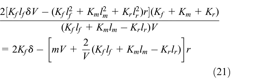
The yaw dynamics equation can be obtained based on the torque balance around the z-axis, as follows:

I_{z} \overset{\cdot}{r} = l_{f} F_{yf} + l_{m} F_{mr} - l_{r} F_{yr}

(12)

By substituting for the lateral force expressions, we then obtain the following relationships:

\begin{matrix} mV \frac{d β}{dt} + 2 (K_{f} + K_{m} + K_{r}) β \\ + [mV + \frac{2}{V} (K_{f} l_{f} + K_{m} l_{m} - K_{r} l_{r})] r \\ = 2 K_{f} δ \end{matrix}

(13)

\begin{matrix} 2 (K_{f} l_{f} + K_{m} l_{m} - K_{r} l_{r}) β + I \frac{dr}{dt} \\ + \frac{2 (K_{f} l_{f}^{2} + K_{m} l_{m}^{2} + K_{r} l_{r}^{2})}{V} r \\ = 2 K_{f} l_{f} δ \end{matrix}

(14)

Equations (13) and (14) are the basic equations of motion required to describe the plane motion of the proposed vehicle. These equations can be written as a state equation model as follows:

\overset{\cdot}{X} = AX + B δ,

(15)

where

\begin{matrix} X = [\begin{matrix} β \\ r \end{matrix}], B = [\begin{matrix} \frac{2 K_{f}}{mV} \\ \frac{2 K_{f} l_{f}}{I} \end{matrix}], \\ A = [\begin{matrix} - \frac{2 (K_{f} + K_{m} + K_{r})}{mV} & - \frac{2 (K_{f} l_{f} + K_{m} l_{m} - K_{r} l_{r})}{m V^{2}} - 1 \\ - \frac{2 (K_{f} l_{f} + K_{m} l_{m} - K_{r} l_{r})}{I} & - \frac{2 (K_{f} l_{f}^{2} + K_{m} l_{m}^{2} + K_{r} l_{r}^{2})}{IV} \end{matrix}] . \end{matrix}

Dynamic equation based on ground coordinate system

During the vehicle steering process, the longitudinal and lateral directions of the vehicle change continuously with respect to the coordinate system fixed to the ground. Therefore, it is convenient to describe the vehicle’s steering motion in a coordinate system that is fixed to the vehicle when traveling along a straight path. As shown in Figure 4, the direction of the straight road surface is the X-axis, and the direction perpendicular to this direction is the Y-axis. The parameter $θ$ represents the angle between the longitudinal direction of the vehicle and the X-axis, $γ$ represents the angle between the vehicle heading and the X-axis, and the lateral displacement of the vehicle’s centre of mass P is denoted by y. When the vehicle is traveling along a straight road, we assume that $| γ | << 1$ and $| θ | << 1$ . Under these assumptions, if the front wheel cornering stiffness $| δ | << 1$ is used, it can then be considered that the directions of the cornering forces F_yf, F_ym, and F_yr that act on the front, middle, and rear wheels, respectively, are the same as the forces acting in the Y direction.

Figure 4.

Vehicle motion in ground coordinate system.

The equation of motion of the vehicle’s centre of mass in the Y direction can then be expressed as follows:

m \frac{d^{2} y}{d t^{2}} = 2 F_{yf} + 2 F_{ym} + 3 F_{yr} .

(16)

The yaw motion of the vehicle can be expressed as follows:

I \frac{d^{2} θ}{d t^{2}} = 2 F_{yf} l_{f} + 2 F_{ym} l_{m} - 2 F_{yr} l_{r} .

(17)

Using the same derivation process that was used for the equation of motion in the vehicle coordinate system, the equation of motion in the ground coordinate system can then be obtained as follows:

\begin{matrix} m \frac{d^{2} y}{d t^{2}} + \frac{2 (K_{f} + K_{m} + K_{r})}{V} \frac{dy}{dt} + \frac{2 (K_{f} l_{f} + K_{m} l_{m} - K_{r} l_{r})}{V} \frac{d θ}{dt} \\ - 2 (K_{f} + K_{m} + K_{r}) θ = 2 K_{f} δ \end{matrix}

(18)

\begin{matrix} \frac{2 (K_{f} l_{f} + K_{m} l_{m} - K_{r} l_{r})}{V} \frac{dy}{dt} + \frac{2 (K_{f} l_{f}^{2} + K_{m} l_{m}^{2} + K_{r} l_{r}^{2})}{V} \frac{d θ}{dt} \\ + I \frac{d^{2} θ}{d t^{2}} - 2 (K_{f} l_{f} + K_{m} l_{m} - K_{r} l_{r}) θ = 2 K_{f} l_{f} δ \end{matrix}

(19)

A Laplace transform can then be obtained from equations (18) and (19), as follows:

\begin{matrix} [\begin{matrix} m s^{2} + \frac{2 (K_{f} + K_{m} + K_{r})}{mV} s & \begin{matrix} \frac{2 (K_{f} l_{f} + K_{m} l_{m} - K_{r} l_{r})}{V} s \\ - 2 (K_{f} + K_{m} + K_{r}) \end{matrix} \\ \frac{2 (K_{f} l_{f} + K_{m} l_{m} - K_{r} l_{r})}{I} s & \begin{matrix} I s^{2} + \frac{2 (K_{f} l_{f}^{2} + K_{m} l_{m}^{2} + K_{r} l_{r}^{2})}{V} s \\ - 2 (K_{f} l_{f} + K_{m} l_{m} - K_{r} l_{r}) \end{matrix} \end{matrix}] [\begin{matrix} y (s) \\ θ (s) \end{matrix}] \\ = [\begin{matrix} 2 K_{f} δ (s) \\ 2 K_{f} l_{f} δ (s) \end{matrix}] \end{matrix}

(20)

Analysis of steerability and handling stability

The handling stability and the steerability are two dynamic vehicle characteristics that are difficult to balance with each other. Oversteer vehicles have high handling stability but poor steerability, while understeer vehicles have high handling stability but poor steerability. This study therefore attempts to solve the contradiction between the handling stability and the steerability by varying the wheelbase to modify the vehicle’s steering characteristics according to the actual demands of driving. To obtain an accurate wheelbase adjustment method, it is necessary to analyse the influence of the change in the wheelbase on the steering performance.

Analysis of steerability

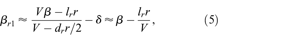
When the vehicle enters a driving state on a smooth curve at a constant speed, $\overset{\cdot}{r} = 0$ and $\overset{\cdot}{β} = 0$ , and these values can then be substituted into equations (13) and (14) to eliminate $β$ . The following formula can thus be obtained:

\begin{matrix} \frac{2 [K_{f} l_{f} δ V - (K_{f} l_{f}^{2} + K_{m} l_{m}^{2} + K_{r} l_{r}^{2}) r] (K_{f} + K_{m} + K_{r})}{(K_{f} l_{f} + K_{m} l_{m} - K_{r} l_{r}) V} \\ = 2 K_{f} δ - [mV + \frac{2}{V} (K_{f} l_{f} + K_{m} l_{m} - K_{r} l_{r})] r \end{matrix}

(21)

After mathematical calculations, the steady-state yaw rate gain is determined as follows:

\begin{matrix} \frac{r}{δ} = [2 K_{f} (K_{f} l_{f} + K_{m} l_{m} - K_{r} l_{r}) V - 2 K_{f} l_{f} (K_{f} + K_{m} + K_{r}) V] \\ / [m V^{2} (K_{f} l_{f} + K_{m} l_{m} - K_{r} l_{r}) + 2 (K_{f} l_{f} + K_{m} l_{m} - K_{r} l_{r})^{2} \\ - 2 (K_{f} + K_{m} + K_{r}) (K_{f} l_{f}^{2} + K_{m} l_{m}^{2} + K_{r} l_{r}^{2})] \end{matrix}

(22)

For the variable-wheelbase vehicle proposed in this paper, it is necessary to specify that l_f and l_r are fixed values during the calculation and do not contain unknown variables. When l_m is to the front of the centre of gravity (CG), it has a positive value, but when the middle axle is to the rear of the CG, l_m has a negative value. Because the value of l_m is variable, the yaw rate gain can be then changed by adjusting the position of the middle axle. As shown in Figure 5, the relationship between the yaw rate gain and the positional adjustment of the middle axle can be obtained by substituting the vehicle’s structural parameters into equation (22) for the numerical calculations.

Figure 5.

Relationship between yaw rate gain and variation of the middle axle position.

The expression for the yaw rate gain can be written as follows:

\frac{r}{δ} = \frac{V / L_{ef}}{1 + K_{us} V^{2}}

(23)

\begin{matrix} K_{us} = [m (K_{f} l_{f} + K_{m} l_{m} - K_{r} l_{r})] / [2 (K_{f} l_{f} + K_{m} l_{m} - K_{r} l_{r})^{2} \\ - 2 (K_{f} {l_{f}}^{2} + K_{m} {l_{m}}^{2} + K_{r} {l_{r}}^{2}) (K_{f} + K_{m} + K_{r})] \end{matrix}

(24)

\begin{matrix} L_{ef} = [(K_{f} {l_{f}}^{2} + K_{m} {l_{m}}^{2} + K_{r} {l_{r}}^{2}) (K_{f} + K_{m} + K_{r}) \\ - (K_{f} l_{f} + K_{m} l_{m} - K_{r} l_{r})^{2}] / [(K_{f} l_{f} + K_{r} l_{r}) (K_{f} + K_{m} + K_{r}) \\ - K_{f} (K_{f} l_{f} + K_{α m} l_{m} - K_{α r} l_{r})] \end{matrix}

(25)

where L_ef is the equivalent wheelbase and K_us is the stability factor. When the expression for K_us is calculated, the denominator is always negative; therefore, the sign of the stability factor K_us is opposite to the sign of the numerator. By substituting the vehicle parameters into equation (24) to perform the numerical calculations, we can obtain the relationship between the stability factor and the middle axle position adjustment, as shown in Figure 6. This figure shows that when the middle axle position is not adjusted, the vehicle then exhibits neutral steering (K_us=0). When the middle axle moves forward (i.e. l_m>0), the vehicle exhibits oversteering (K_us<0) and when the middle axle moves backward (i.e. l_m<0), the vehicle then exhibits understeering (K_us>0). The relationship between the equivalent wheelbase and the middle axle adjustment is shown in Figure 7. When the middle axle is in its initial position, the equivalent wheelbase has the smallest value, and as the wheelbase adjustment increases in either direction, the equivalent wheelbase value increases.

Figure 6.

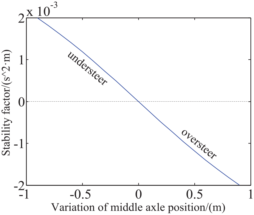
Relationship between stability factor and variation of the middle axle position.

Figure 7.

Relationship between effective wheelbase and variation of the middle axle position.

Analysis of handling stability

The vehicle motion characteristics can be obtained from equation (20), as follows:

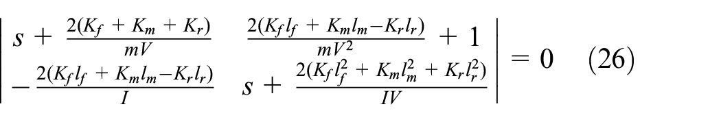
| \begin{matrix} s + \frac{2 (K_{f} + K_{m} + K_{r})}{mV} & \frac{2 (K_{f} l_{f} + K_{m} l_{m} - K_{r} l_{r})}{m V^{2}} + 1 \\ - \frac{2 (K_{f} l_{f} + K_{m} l_{m} - K_{r} l_{r})}{I} & s + \frac{2 (K_{f} l_{f}^{2} + K_{m} l_{m}^{2} + K_{r} l_{r}^{2})}{IV} \end{matrix} | = 0

(26)

Equation (26) can then be expressed as follows:

s^{2} + 2 ξ ω_{n} s + {ω_{n}}^{2} = 0

(27)

Equation (27) is the characteristic equation of the system, where the following relationships hold:

2 ξ ω_{n} = \frac{2 K_{f} + 2 K_{m} + 2 K_{r}}{mV} + \frac{2 K_{f} {l_{f}}^{2} + 2 K_{m} {l_{m}}^{2} + 2 K_{r} {l_{r}}^{2}}{IV}

(28)

\begin{matrix} {ω_{n}}^{2} = \frac{4 (K_{f} + K_{m} + K_{r}) (K_{f} {l_{f}}^{2} + K_{m} {l_{m}}^{2} + K_{r} {l_{r}}^{2})}{mI V^{2}} \\ - \frac{2 (m V^{2} + 2 K_{f} l_{f} + 2 K_{m} l_{m} - 2 K_{r} l_{r}) (K_{f} l_{f} + K_{m} l_{m} - K_{r} l_{r})}{mI V^{2}} \end{matrix}

(29)

The system is represented by the characteristic equation (27), which gives a response that can be represented by $C_{1} e^{λ_{1} t} + C_{2} e^{λ_{2} t}$ , where $λ_{1}$ and $λ_{2}$ are the roots of the characteristic equation (26), as follows:

λ_{1, 2} = - ξ ω_{n} \pm \sqrt{{(ξ ω_{n})}^{2} - {ω_{n}}^{2}}

(30)

The system’s transient response characteristics and its stability both depend on the root of the characteristic equation. Therefore, the transient response characteristics and the stability of the vehicle can be classified as follows, using the values of $ξ ω_{n}$ and ${ω_{n}}^{2}$ :

1) If $(ξ ω_{n})^{2} - {ω_{n}}^{2} \geq 0$ and ${ω_{n}}^{2} > 0$ , then $λ_{1}$ and $λ_{2}$ are negative real numbers; therefore, the vehicle has a transient response composed of undamped oscillation (system stability).

2) If $(ξ ω_{n})^{2} - {ω_{n}}^{2} < 0$ , then $λ_{1}$ and $λ_{2}$ are complex numbers, but if their real parts are negative, the transient response is oscillating attenuation (system stability).

3) If ${ω_{n}}^{2} < 0$ , then either $λ_{1}$ or $λ_{2}$ is a negative real number; because one value is a positive real number, the transient response is non-oscillating divergence (system instability).

Therefore, ${ω_{n}}^{2} > 0$ defines the condition for system stability, and equation (29) can be converted into the following equation:

\begin{matrix} \frac{(m V^{2} + 2 K_{f} l_{f} + 2 K_{m} l_{m} - 2 K_{r} l_{r}) (K_{f} l_{f} + K_{m} l_{m} - K_{r} l_{r})}{(K_{f} + K_{m} + K_{r})} \\ \leq 2 (K_{f} {l_{f}}^{2} + K_{m} {l_{m}}^{2} + K_{r} {l_{r}}^{2}) \end{matrix}

(31)

Equation (31) can be satisfied if $l_{m} \leq 0$ ; therefore, the system is in a steady state when the middle axle moves backward, and the critical speed thus only considers the case where $l_{m} > 0$ . If ${ω_{n}}^{2} = 0$ , the critical speed can be obtained as follows:

V_{c} = \sqrt{\frac{2 (K_{f} + K_{m} + K_{r}) (K_{f} {l_{f}}^{2} + K_{m} {l_{m}}^{2} + K_{r} {l_{r}}^{2})}{\begin{matrix} m (K_{f} l_{f} + K_{m} l_{m} - K_{r} l_{r}) \\ - \frac{2}{m} (K_{f} l_{f} + K_{m} l_{m} - K_{r} l_{r}) \end{matrix}}}

(32)

By substituting the vehicle parameters from Table 1 into equation (32), the relationship between the critical velocity and the variation of the middle axle position can be obtained as shown in Figure 8. As the figure shows, the critical speed decreases as the middle axle moves further forward. This indicates that the vehicle’s traveling stability is weaker, which is consistent with the yaw rate gain case shown in Figure 5. Additionally, Figure 5 shows that the yaw rate gain increases as the middle axle moves further forward; i.e., when the middle axle moves forward, the steerability of the vehicle is enhanced but its stability degrades. Similarly, Figure 8 is also consistent with Figure 6, which indicates that the stability factor tends to become negative when the middle axle moves forward.

Figure 8.

Relationship between critical velocity and variation of the middle axle position.

Analysis of Steering Error

Steering stability and lane-keeping are two major problems in vehicle steering control.²¹ The steering stability of a three-axle vehicle with a variable wheelbase was investigated as described above. This section describes the investigation with regard to the effect of the variable wheelbase on the vehicle’s lane-keeping ability. Two new variables are defined for the lateral dynamics model here: the distance from the centreline of the lane to the CG of the vehicle e₁, and the vehicle directional error relative to the lane e₂. If the vehicle is assumed to travel at a constant longitudinal speed on a curved road with a large radius R, the theoretical rate of directional change of the vehicle is defined as:

r_{des} = \frac{V}{R}

(33)

The theoretical acceleration of the vehicle can then be expressed as:

\frac{V^{2}}{R} = V r_{des}

(34)

Therefore,

{\overset{\cdot\cdot}{e}}_{1} = (V \frac{d β}{dt} + Vr) - \frac{V^{2}}{R}, e_{2} = ψ - ψ_{des} .

(35)

Using equations (34) and (35), equations (13) and (14) can be converted as follows:

\begin{matrix} m {\overset{\cdot\cdot}{e}}_{1} = - \frac{2}{V} (K_{f} + K_{m} + K_{r}) {\overset{\cdot}{e}}_{1} \\ - \frac{2}{V} (K_{f} l_{f} + K_{m} l_{m} - K_{r} l_{r}) {\overset{\cdot}{e}}_{2} \\ + 2 (K_{f} + K_{m} + K_{r}) e_{2} \\ - [\frac{2}{V} (K_{f} l_{f} + K_{m} l_{m} - K_{r} l_{r}) + V] r_{des} \\ + 2 K_{f} δ \end{matrix}

(36)

\begin{matrix} I {\overset{\cdot\cdot}{e}}_{2} = - \frac{2}{V} (K_{f} l_{f} + K_{m} l_{m} - K_{r} l_{r}) {\overset{\cdot}{e}}_{1} \\ + 2 (K_{f} l_{f} + K_{m} l_{m} - K_{r} l_{r}) e_{2} \\ + 2 (K_{f} l_{f} + K_{r} l_{r}) δ - \frac{2}{V} (K_{f} {l_{f}}^{2} + K_{m} {l_{m}}^{2} + K_{r} {l_{r}}^{2}) {\overset{\cdot}{e}}_{2} \\ - \frac{2}{V} (K_{f} {l_{f}}^{2} + K_{m} {l_{m}}^{2} + K_{r} {l_{r}}^{2}) r_{des} \end{matrix}

(37)

The state model of the tracking error can be expressed as:

\overset{\cdot}{x} = Ax + B_{1} δ + B_{2} {\overset{\cdot}{ψ}}_{des},

(38)

where $x = {[\begin{matrix} e_{1} & {\overset{\cdot}{e}}_{1} & e_{2} & {\overset{\cdot}{e}}_{2} \end{matrix}]}^{T} .$

The open-loop matrix A has two unstable eigenvalues and the system requires feedback to stabilize the matrix. The state feedback rule is used here as follows:

δ = - Kx + δ_{ff} = - k_{1} e_{1} - k_{2} {\overset{\cdot}{e}}_{1} - k_{3} e_{2} - k_{4} {\overset{\cdot}{e}}_{2} + δ_{ff} .

(39)

The state space model of the closed-loop lateral control system can be expressed as:

\overset{\cdot}{x} = (A - B_{1} K) x + B_{1} δ_{ff} + B_{2} r_{des} .

(40)

If the system’s initial state is 0, then the Laplace transform can be used to convert equation (40) as follows:

X (s) = [sI - (A - B_{1} K)]^{- 1} {B_{1} L (δ_{ff}) + B_{2} L (r_{des})}

(41)

Application of the final value theorem allows the steady-state tracking error to be expressed as:

x_{ss} = lim_{t \to \infty} x (t) = lim_{s \to 0} sX (s) = - (A - B_{1} K)^{- 1} {B_{1} δ_{ss} + B_{2} \frac{V}{R}}

(42)

After various mathematical operations are performed, the final form of the steady-state tracking error can be expressed as follows:

x_{ss} = {[\begin{matrix} f (k_{1}, k_{3}, δ_{ff}) & 0 & f (C, m, R, l, V) & 0 \end{matrix}]}^{T},

(43)

where

\begin{matrix} f (C, m, R, l, V) = [m V^{2} (K_{f} l_{f} + K_{r} l_{r}) + 2 K_{m} K_{f} l_{m} (l_{f} - l_{m}) \\ + 2 K_{m} K_{r} l_{m} (l_{r} + l_{m}) + 2 K_{f} K_{r} l (l_{f} - l_{r})] \\ / [2 R K_{f} K_{m} (l_{f} - l_{m}) + 4 R K_{f} K_{r} l + 2 R K_{m} K_{r} (l_{r} + l_{m})] \end{matrix}

(44)

From equation (43), it is known that the lateral position error can be set at 0 by setting an appropriate value for the state feedback matrix. However, K does not affect the steady-state angular error. The steady-state angular error can be expressed as:

\begin{matrix} e_{2 ss} = [m V^{2} (K_{f} l_{f} + K_{r} l_{r}) + 2 K_{m} K_{f} l_{m} (l_{f} - l_{m}) \\ + 2 K_{m} K_{r} l_{m} (l_{r} + l_{m}) + 2 K_{f} K_{r} l (l_{f} - l_{r})] \\ / [2 R K_{f} K_{m} (l_{f} - l_{m}) + 4 R K_{f} K_{r} l + 2 R K_{m} K_{r} (l_{r} + l_{m})] \end{matrix}

(45)

If $K_{m} = K_{f} = K_{r}$ , then equation (44) can be simplified as follows:

e_{2 ss} = \frac{m V^{2}}{6 R K_{f}} + \frac{l_{m} + l_{f} - l_{r}}{3 R} .

(46)

The analysis above shows that an error in the steady-state direction angle always exists as a fixed value for vehicles with an invariable structural parameter. However, in the proposed variable-wheelbase vehicle, the direction angle error during steady-state steering can be reduced by adjusting the middle axle position to enhance the lane-keeping ability of the vehicle. Figure 9 shows the relationship between the variation of the middle axle position and the direction angle error, which can be obtained by substituting the vehicle parameters given in Table 1 into equation (46). The magnitude of the steady-state direction error varies with changes in the middle axle position. The direction angle error is reduced significantly when l_m changes from a positive to a negative value. The steady-state direction angle error is 4.4° when l_m is 0, but the steady-state direction angle error is reduced to 3.2° after the middle axle moves backward by 0.5 m, and when the middle axle moves further back, the direction angle error continues to decrease in a linear manner.

Figure 9.

Steady-state steering direction angle error.

Analysis of lateral anti-disturbance resistance

The previous section discussed the vehicle motion characteristics under the control input. In the absence of the steering input, the vehicle should theoretically maintain a straight-line driving state. However, under actual driving conditions, the vehicle will inevitably be subject to external disturbances, e.g. wind, and undesired motion. This section describes the vehicle motion under the action of external lateral forces to enable further analysis of the characteristics of the vehicle dynamics.

Vehicle motion under stepped lateral force

When a vehicle is traveling on an inclined road surface, the lateral component of its force due to gravity becomes the lateral force Y acting on the vehicle’s centre of mass, as shown in Figure 10. If the vehicle travels on a slope for a long time, i.e., if the lateral disturbance force Y is exerted for a long time, the vehicle will deviate from its original path even if this force is small.

Figure 10.

Vehicle being subjected to lateral force.

Assuming that the steering angle of the vehicle is 0°, then according to equations (13) and (14), the equation of motion of the vehicle under the action of the lateral force can be expressed as:

\begin{matrix} mV \frac{d β}{dt} + 2 (K_{f} + K_{m} + K_{r}) β \\ + [mV + \frac{2}{V} (K_{f} l_{f} + K_{m} l_{m} - K_{r} l_{r})] r = Y \end{matrix}

(47)

\begin{matrix} 2 (K_{f} l_{f} + K_{m} l_{m} - K_{r} l_{r}) β + I \frac{dr}{dt} \\ + \frac{2 (K_{f} l_{f}^{2} + K_{m} l_{m}^{2} + K_{r} l_{r}^{2})}{V} r \\ = 0 \end{matrix}

(48)

By performing Laplace transforms on equations (47) and (48), the responses of the vehicle’s yaw angle $β (s)$ and yaw rate r(s) to the action of the lateral force Y can be obtained as follows:

\begin{matrix} β (s) = \frac{| \begin{matrix} \frac{Y_{0}}{s} & mV + \frac{2}{V} (K_{f} l_{f} + K_{m} l_{m} - K_{r} l_{r}) \\ 0 & Is + \frac{2 (K_{f} l_{f}^{2} + K_{m} l_{m}^{2} + K_{r} l_{r}^{2})}{V} \end{matrix} |}{| \begin{matrix} mVs + 2 (K_{f} + K_{m} + K_{r}) & mV + \frac{2}{V} (K_{f} l_{f} + K_{m} l_{m} - K_{r} l_{r}) \\ 2 (K_{f} l_{f} + K_{m} l_{m} - K_{r} l_{r}) & Is + \frac{2 (K_{f} l_{f}^{2} + K_{m} l_{m}^{2} + K_{r} l_{r}^{2})}{V} \end{matrix} |} \\ = \frac{Y_{0}}{mVs} \frac{(s + a_{β})}{(s^{2} + 2 ξ ω_{n} s + ω_{n}^{2})} \end{matrix}

(49)

\begin{matrix} r (s) = \frac{| \begin{matrix} mVs + 2 (K_{f} + K_{m} + K_{r}) & \frac{Y_{0}}{s} \\ 2 (K_{f} l_{f} + K_{m} l_{m} - K_{r} l_{r}) & 0 \end{matrix} |}{| \begin{matrix} mVs + 2 (K_{f} + K_{m} + K_{r}) & mV + \frac{2}{V} (K_{f} l_{f} + K_{m} l_{m} - K_{r} l_{r}) \\ 2 (K_{f} l_{f} + K_{m} l_{m} - K_{r} l_{r}) & Is + \frac{2 (K_{f} l_{f}^{2} + K_{m} l_{m}^{2} + K_{r} l_{r}^{2})}{V} \end{matrix} |} \\ = \frac{Y_{0}}{mVIs} \frac{a_{r}}{(s^{2} + 2 ξ ω_{n} s + ω_{n}^{2})} \end{matrix}

(50)

where

\begin{matrix} a_{β} = \frac{2 (K_{f} l_{f}^{2} + K_{m} l_{m}^{2} + K_{r} l_{r}^{2})}{VI} \\ a_{r} = - 2 (K_{f} l_{f} + K_{m} l_{m} - K_{r} l_{r}) . \end{matrix}

(51)

The parameters $ξ$ and $ω_{n}$ are given by equations (28) and (29), respectively, and Y₀/s is the Laplace transform of the lateral force Y. The steady-state values of $β (s)$ and r(s) can then be calculated using the final value theorem Laplace transform, as follows:

\begin{matrix} β = lim_{s \to 0} s β (s) = \frac{Y_{0}}{mV} \frac{a_{β}}{ω_{n}^{2}} \\ = \frac{2 Y_{0}}{mI V^{2} ω_{n}^{2}} (K_{f} l_{f}^{2} + K_{m} l_{m}^{2} + K_{r} l_{r}^{2}), \end{matrix}

(52)

\begin{matrix} r = lim_{s \to 0} sr (s) = \frac{Y_{0}}{mIV} \frac{a_{r}}{ω_{n}^{2}} \\ = \frac{- 2 Y_{0}}{mI V^{2} ω_{n}^{2}} (K_{f} l_{f} + K_{m} l_{m} - K_{r} l_{r}) . \end{matrix}

(53)

The previous analysis showed that the vehicle driving direction remains stable when the vehicle speed is lower than the critical speed ( ${ω_{n}}^{2} \geq 0$ ). According to equation (52), $β$ is always positive. In other words, r has the same sign as the stability factor K_us (where K_us and K_f have opposite signs). Therefore, r is positive when the vehicle is in understeer, but r is negative when the vehicle is in oversteer.

To calculate the values of equations (52) and (53), we constructed the numerical calculation model shown in Figure 11. The model input was the lateral force step input, which occurs at 0.5 s, and where the lateral force is 4,000 N and the vehicle is traveling at 40 km/h. The steering angle was 0° and the model simulated the response of the vehicle when subjected to a stepped lateral force, whereby the force increases only once.

Figure 11.

Numerical calculation model developed in Simulink.

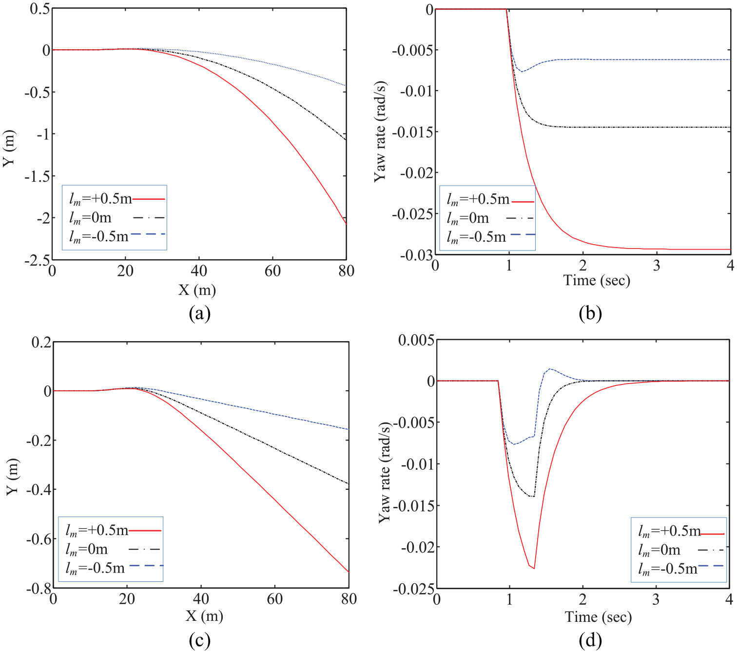
The run time for the numerical calculation model was 4 s, and the vehicle yaw rate and the CG position change are shown in Figure 12(a) and (b), respectively. As the figure shows, the yaw rate increased rapidly from 0 when the vehicle was subjected to the lateral force at 0.5 s. The yaw rate reached a steady value after 1 s, which indicates that the vehicle had entered a steady state. With this yaw motion, the lateral position of the vehicle also changed; the vehicle shifted to one side and the offset increased over time.

Figure 12.

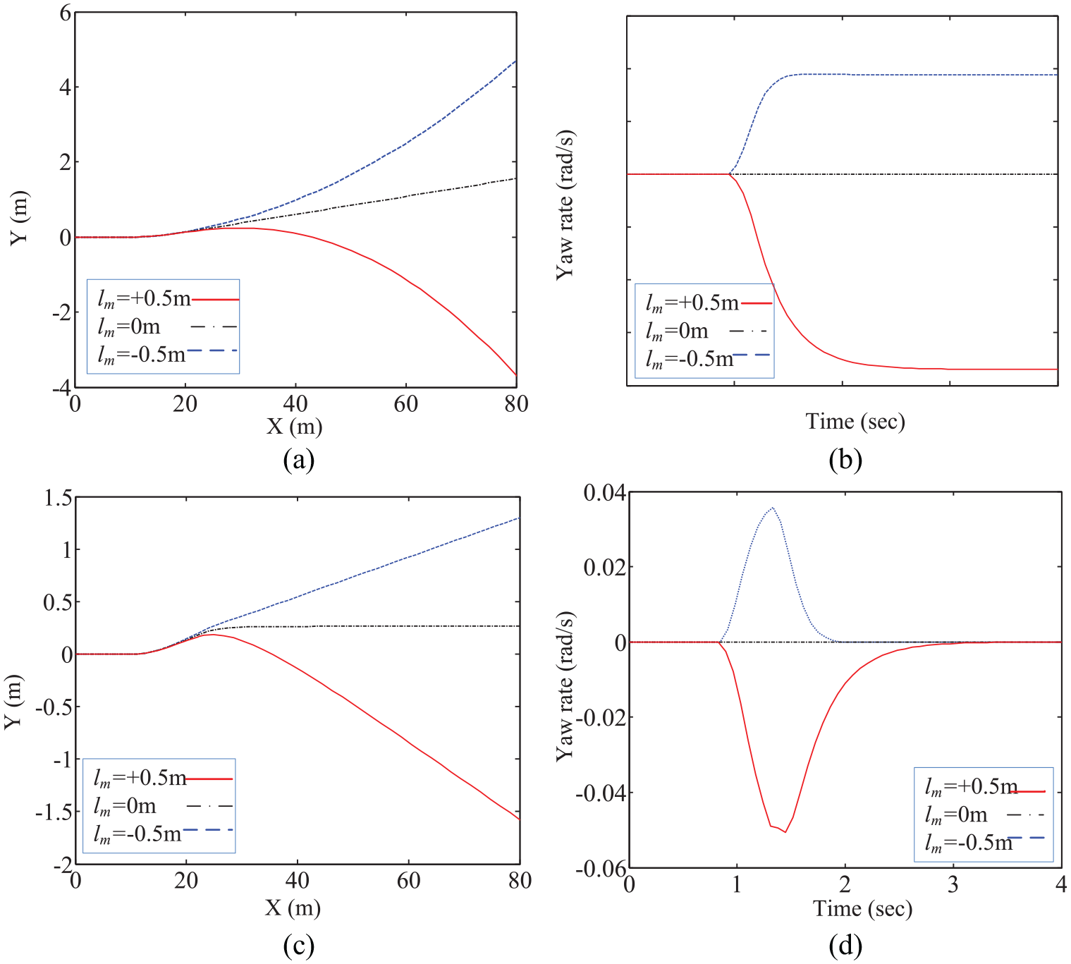
Vehicle responses under the action of lateral forces: (a) position of CG under stepped force; (b) vehicle yaw rate under stepped force; (c) position of CG under pulsed force; (d) vehicle yaw rate under pulsed force.

Figure 12 shows that the yaw rate was lowest when the middle axle was in the initial position, while the yaw rate was highest when the middle axle was in its forward-most position with the lateral stepped force acting on the CG. Therefore, the vehicle has better anti-disturbance resistance when the middle axle is in its initial position because this position creates neutral vehicle steer. In this situation, the lateral disturbance acting on the centre of mass of the vehicle and the lateral force from the tyres do not generate a yaw moment around the centre of mass of the vehicle. When the middle axle is not in its initial position, the vehicle is in either understeer or oversteer, and the neutral turning point then no longer coincides with the centre of mass. The lateral disturbance force and the lateral force of the tyre will then produce a yaw moment that increases the yaw motion of the vehicle.

Vehicle motion under pulsed lateral force

In the previous section, we discussed the case of a stepped lateral force acting on the vehicle. However, such a continuously applied force is unlikely in the real world, so in this section, we discuss the case of a discontinuous pulsed force acting on the vehicle. This represents a more practical situation for a vehicle traveling on a partially inclined road. We assume that the time $Y_{0} Δ t$ for which the pulsed lateral force acts on the vehicle is not large and that the vehicle does not deviate very far from its original path under the action of the pulsed force. Therefore, it is more convenient to use the ground coordinate system to describe the vehicle’s movement. When the vehicle is traveling in a straight line, then according to equations (18) and (19), the equation of motion for the vehicle under the action of the pulsed lateral force can be expressed as follows:

\begin{matrix} m \frac{d^{2} y}{d t^{2}} + \frac{2 (K_{f} + K_{m} + K_{r})}{V} \frac{dy}{dt} \\ + \frac{2 (K_{f} l_{f} + K_{m} l_{m} - K_{r} l_{r})}{V} \frac{d θ}{dt} \\ - 2 (K_{f} + K_{m} + K_{r}) θ = Y \end{matrix}

(54)

\begin{matrix} \frac{2 (K_{f} l_{f} + K_{m} l_{m} - K_{r} l_{r})}{V} \frac{dy}{dt} \\ + \frac{2 (K_{f} l_{f}^{2} + K_{m} l_{m}^{2} + K_{r} l_{r}^{2})}{V} \frac{d θ}{dt} \\ + I \frac{d^{2} θ}{d t^{2}} - 2 (K_{f} l_{f} + K_{m} l_{m} - K_{r} l_{r}) θ = 0 \end{matrix}

(55)

When $Δ t$ is much smaller than the period in which the vehicle’s motion changes, the approximate Laplace transform of the lateral force Y can be recorded as $Y_{0} Δ t$ . Therefore, the vehicle’s response to the pulsed lateral force can be obtained by performing Laplace transforms on equations (54) and (55).

y (s) = \frac{Y Δ t}{m} \frac{s^{2} + a_{y 1} s + a_{y 2}}{s^{2} (s^{2} + 2 ξ' {ω_{n}}^{'} s + ω_{n}'^{2})},

(56)

θ (s) = \frac{Y Δ t}{mIVs} \frac{a_{r}}{s^{2} (s^{2} + 2 ξ' {ω_{n}}^{'} s + ω_{n}'^{2})},

(57)

where

\begin{matrix} a_{y 1} = \frac{2 (K_{f} l_{f}^{2} + K_{m} l_{m}^{2} + K_{r} l_{r}^{2})}{IV} \\ a_{y 2} = - \frac{2 (K_{f} l_{f} + K_{m} l_{m} - K_{r} l_{r})}{I} \\ a_{r} = - 2 (K_{f} l_{f} + K_{m} l_{m} - K_{r} l_{r}) \\ {ω_{n}}^{'} = \sqrt{\frac{4 (K_{f} + K_{m} + K_{r}) (K_{f} l_{f}^{2} + K_{m} l_{m}^{2} + K_{r} l_{r}^{2})}{\begin{matrix} mI V^{2} \\ - \frac{4 {(K_{f} l_{f} + K_{m} l_{m} - K_{r} l_{r})}^{2}}{mI V^{2}} - \frac{2 (K_{f} l_{f} + K_{m} l_{m} - K_{r} l_{r})}{I} \end{matrix}}} \end{matrix}

(58)

and

ξ' {ω_{n}}^{'} = \frac{(K_{f} l_{f}^{2} + K_{m} l_{m}^{2} + K_{r} l_{r}^{2}) + I (K_{f} + K_{m} + K_{r})}{mIV} .

(59)

The final value theorem of the Laplace transform can then be used to obtain the steady-state values of the lateral displacement of the CG, and the vehicle’s longitudinal direction angle can also be obtained.

If $K_{f} l_{f} + K_{m} l_{m} - K_{r} l_{r} = 0,$ then

\begin{matrix} y = lim_{s \to 0} sy (s) \\ = \frac{Y_{0} V Δ t (K_{f} l_{f}^{2} + K_{m} l_{m}^{2} + K_{r} l_{r}^{2})}{2 (K_{f} + K_{m} + K_{r}) (K_{f} l_{f}^{2} + K_{m} l_{m}^{2} + K_{r} l_{r}^{2}) - 2 {(K_{f} l_{f} + K_{m} l_{m} - K_{r} l_{r})}^{2}} \end{matrix}

(60)

If $K_{f} l_{f} + K_{m} l_{m} - K_{r} l_{r} \neq 0,$ then

\begin{matrix} y = lim_{s \to 0} sy (s) = \pm \infty \\ θ = lim_{s \to 0} s θ (s) = [- Y_{0} V Δ t (K_{f} l_{f} + K_{m} l_{m} - K_{r} l_{r})] / \\ [2 (K_{f} + K_{m} + K_{r}) (K_{f} l_{f}^{2} + K_{m} l_{m}^{2} + K_{r} l_{r}^{2}) \\ - 2 (K_{f} l_{f} + K_{m} l_{m} - K_{r} l_{r})^{2} \\ - m V^{2} (K_{f} l_{f} + K_{m} l_{m} - K_{r} l_{r})] \end{matrix}

(61)

From equations (60) and (61), it can be seen that $y = + \infty$ and $θ$ has a positive value under the action of the pulsed lateral force when the vehicle tends to understeer (where $K_{f} l_{f} + K_{m} l_{m} - K_{r} l_{r} < 0$ ). If $K_{f} l_{f} + K_{m} l_{m} - K_{r} l_{r} > 0$ , the vehicle then tends to oversteer under the action of the pulsed lateral force and $θ$ has a negative value such that $y = - \infty$ . If $K_{f} l_{f} + K_{m} l_{m} - K_{r} l_{r} = 0$ , the vehicle is in the neutral steering mode, y has a positive value, and $θ$ is 0.

Figure 12(c) and (d) present the results obtained from the calculation model after the input signal of the Simulink model was changed to a pulsed input signal. The figure shows that the response to the pulsed lateral force is similar to the response to the stepped lateral force. When the middle axle is in its initial position, the lateral disturbance force then has the lowest influence on the vehicle motion. The effect of the force is greatest when the middle axle is at its forward-most position. The pulsed force response differs from the stepped force response in that the vehicle’s yaw rate tends toward zero over time, and the vehicle’s travel direction remains in a straight line. For the stepped response, the yaw angular velocity only converges to zero when the middle axle is in its initial position. The vehicle’s yaw angular velocity tends toward stability when the middle axle is at a different position, and the vehicle then travels along a curved path.

Therefore, when the vehicle is subjected to the lateral pulsed force, the wheelbase change strategy can be derived as follows: the middle axle should be kept at its initial position when the vehicle is subjected to a lateral disturbance to minimize the effect of this disturbance on the vehicle’s motion.

Vehicle motion under lateral wind

If the vehicle is subjected to the force of a lateral wind during high-speed driving, the vehicle will then produce a lateral motion. If the vehicle is traveling in a straight line at a speed V and is then subjected to a lateral wind of speed w, the lateral force Y_w and the yaw moment N_w acting on the vehicle are then expressed as follows:

Y_{w} = C_{y} \frac{ρ}{2} S (V^{2} + w^{2}),

(62)

N_{w} = C_{n} \frac{ρ}{2} lS (V^{2} + w^{2}),

(63)

where C_y is the lateral force coefficient, C_n is the yaw moment coefficient (with the positive value of C_n being defined in the anticlockwise direction), $ρ$ is the air density, S is the windward area of the vehicle, and l is the vehicle’s wheelbase. Both C_y and C_n are functions of the side-slip angle of the airflow. The point of action of the lateral force Y_w is called the aerodynamic centre (AC). The distance between the AC and the CG is l_w, and the AC is defined as positive when it is behind the CG. Therefore, the yaw moment N_w that acts on the vehicle can be expressed as follows:

N_{w} = - l_{w} Y_{w} .

(64)

When the vehicle is subjected to a constant crosswind, the lateral force Y_w generated by this crosswind is assumed to be a stepped force and acts on the AC of the vehicle. The vehicle’s motion is then expressed in the vehicle coordinate system as:

\begin{matrix} [mV + \frac{2}{V} (K_{f} l_{f} + K_{m} l_{m} - K_{r} l_{r})] r + 2 (K_{f} + K_{m} + K_{r}) β \\ + mV \frac{d β}{dt} = Y_{w} \end{matrix}

(65)

\begin{matrix} \frac{2 (K_{f} l_{f}^{2} + K_{m} l_{m}^{2} + K_{r} l_{r}^{2})}{V} r + 2 (K_{f} l_{f} + K_{m} l_{m} - K_{r} l_{r}) β \\ + I \frac{dr}{dt} = - l_{w} Y_{w} \end{matrix}

(66)

Similarly, the steady-state values of $β$ and r can be obtained using the Laplace transform, as follows:

\begin{matrix} β = \frac{2 (K_{f} l_{f}^{2} + K_{m} l_{m}^{2} + K_{r} l_{r}^{2})}{mI V^{2} ω_{n}^{2}} Y_{w 0} \\ - \frac{2 l_{w} l_{N} (K_{f} + K_{m} + K_{r}) + m l_{w} V^{2}}{mI V^{2} ω_{n}^{2}} Y_{w 0} \end{matrix}

(67)

r = \frac{2 (l_{N} - l_{w}) (K_{f} + K_{m} + K_{r}) V}{mI V^{2} ω_{n}^{2}} Y_{w 0}

(68)

where

l_{N} = - \frac{K_{f} l_{f} + K_{m} l_{m} - K_{r} l_{r}}{K_{f} + K_{m} + K_{r}} .

(69)

As shown by the analysis of the handling stability, if the vehicle travel speed is less than the critical speed, then $ω_{n}^{2} > 0$ , so the sign of r is dependent on the sign obtained for l_N−l_w: if l_N>l_w, then r>0; if l_N<l_w, then r<0; and if l_N=l_w, then r=0. Using the steady-state value of the yaw rate, the steady-state lateral acceleration caused by the action of the side wind can be calculated as follows:

S_{w} = \frac{2 (l_{N} - l_{w}) (K_{f} + K_{m} + K_{r}) V^{2}}{mI V^{2} ω_{n}^{2}}

(70)

S_w is thus called the crosswind sensitivity coefficient and is used as an indicator of the vehicle’s sensitivity to crosswind disturbances.

The same numerical calculation model was then used to vary the force and the torque input, given by l_w = −0.4. As shown in Figure 13, the vehicle’s motion response under the action of a lateral constant wind is calculated. Figure 13(a) shows the trajectory of the CG. It can be seen from this figure that the crosswind sensitivity is at its lowest and the lateral position offset is at its smallest when the middle axle is in its hindmost position. However, the vehicle deviation is most pronounced when the middle axle is in its forward-most position. Figure 13(b) shows that the yaw rate will eventually maintain a nonzero steady-state value under the influence of a constant crosswind, regardless of the positioning of the middle axle, and the vehicle will then travel along a curved path. As the middle axle position moves further rearward, the steady-state value of the yaw rate decreases, the lateral displacement of the vehicle per unit time also decreases, and the radius of the curved path increases.

Figure 13.

Vehicle responses under the action of steady and gusting lateral winds: (a) position of CG under steady wind; (b) vehicle yaw rate under steady wind; (c) position of CG under gusting wind; (d) vehicle yaw rate under gusting wind.

Next, we consider the case where the vehicle is subjected to a short lateral gust and the steering angle of the vehicle is 0°. If the gust duration is sufficiently small, the gust can be considered to be a pulsed input. The absolute coordinate system fixed to the ground is then used to describe the vehicle motion.

\begin{matrix} m \frac{d^{2} y}{d t^{2}} + \frac{2 (K_{f} + K_{m} + K_{r})}{V} \frac{dy}{dt} \\ + \frac{2 (K_{f} l_{f} + K_{m} l_{m} - K_{r} l_{r})}{V} \frac{d θ}{dt} \\ - 2 (K_{f} + K_{m} + K_{r}) θ = Y_{w} \end{matrix}

(71)

\begin{matrix} \frac{2 (K_{f} l_{f} + K_{m} l_{m} - K_{r} l_{r})}{V} \frac{dy}{dt} \\ + \frac{2 (K_{f} l_{f}^{2} + K_{m} l_{m}^{2} + K_{r} l_{r}^{2})}{V} \frac{d θ}{dt} \\ + I \frac{d^{2} θ}{d t^{2}} - 2 (K_{f} l_{f} + K_{m} l_{m} - K_{r} l_{r}) θ = - l_{w} Y_{w} \end{matrix}

(72)

The steady-state values of the vehicle’s lateral position and heading angle can then be obtained by performing a Laplace transform, as follows:

y = \pm \infty (l_{N} \neq l_{w}) .

(73)

However, if $l_{N} = l_{w},$ then

y = \frac{2 (K_{f} l_{f}^{2} + K_{m} l_{m}^{2} + K_{r} l_{r}^{2}) - 2 l_{w} l_{N} (K_{f} + K_{m} + K_{r})}{mIV ω_{n}^{2}} Y_{w 0} Δ t

(74)

θ = \frac{2 (l_{N} - l_{w}) (K_{f} + K_{m} + K_{r})}{mIV ω_{n}^{2}} Y_{w 0} Δ t .

(75)

When the vehicle speed is lower than the critical speed, the steady-state motion of the vehicle can be summarized as follows. If l_N>l_w, $y = + \infty$ , and $θ$ is a positive constant; if l_N=l_w, y is a positive constant and $θ = 0$ . Additionally, if l_N<l_w, $y = - \infty$ , and $θ$ is a negative constant. The numerical calculation results for the vehicle moving under the action of the lateral gust are shown in Figure 13(c). Similar to the effect of the lateral constant wind, the vehicle is least affected by the lateral gust when the middle axle is at its rearmost position, and most strongly affected when the middle axle is in the front position. In contrast with effect of the lateral constant wind, the steady-state values of the vehicle yaw rate are all zero at the different wheelbase lengths when the vehicle is subjected to the lateral gust (Figure 13(d)). Therefore, the vehicle will eventually travel in a straight line. When the middle axle is at its rearmost position, the peak yaw rate value is at its smallest and the yaw rate’s sensitivity to the lateral gust is also at its smallest.

Therefore, the wheelbase adjustment strategy for the action of lateral winds can be obtained as follows. When the vehicle is driving on a windy road, the middle axle should be adjusted to be at its rearmost position to reduce the vehicle’s sensitivity to the lateral wind and to enhance the driving stability and the ground tracking capability.

Simulation

Simulation of handling stability

To verify the theoretical calculation results, a three-dimensional model of the proposed vehicle was imported into the ADAMS simulation program. The road spectrum function was used to simulate a smooth road surface and a tyre model with constant vertical stiffness and cornering stiffness was built. The front and rear steering wheels were both assigned an angle of 8° at 3 s, and the vehicle travel speed was maintained at 50 km/h during the simulation. Three different middle axle positions were simulated: moved forward by 0.5 m, moved backward by 0.5 m, and the initial position.

The trajectories of the vehicle in these three cases are shown in Figure 14, which shows that the vehicle tends to have a larger steering radius when the middle axle is moved backward. It can also be observed from the motion trajectory shown in Figure 14 that the vehicle tends to understeer when the middle axle is moved backward, while the vehicle tends to oversteer when the middle axle is moved forward. Therefore, yaw control can be realized by varying the position of the middle axle.

Figure 14.

Steering tracks produced by three simulations of the middle axle position.

When compared with the middle axle at the front end or rear end positions, the middle axle at the initial position is in a transitional state. To simplify the comparison of the simulation results, only the simulation results for the middle axle at the front end and the middle axle at the rear end are selected. The difference in the CG positions between the cases of forward and backward movement of the middle axle is shown in Figure 15(a), which shows that the steering radius of the vehicle is different in the two cases and indicates that the steering radius differs by approximately 5 m between the two cases. The vehicle will have a greater turning radius if the middle axle is moved backward. Figure 15(b) shows the yaw rate response of the vehicle. The yaw rate increases rapidly to a peak value of 45°/s after the angle signal is input at 3 s, and a steady state is reached at 4.6 s. The yaw rates of the two simulations have the same variance trend, the same peak value, and the same response time. The main difference is that the vehicle has a different yaw rate in the steady state. The steady-state yaw rate after the middle axle is moved forward is greater than the steady-state yaw rate when the axle is moved backward. Figure 15(c) shows the lateral acceleration during the vehicle’s operation. The vehicle is traveling in a straight line during the first 3 s and thus the lateral acceleration in these first 3 s is zero. The vehicle with the middle axle in the forward position shows a larger lateral acceleration. As shown in Figure 15(d), the side-slip angle of the rear axle wheel is greater when the middle axle is moved forward, which increases the vehicle oversteering tendency and reduces the steering radius.

Figure 15.

Simulation results for the steering: (a) position of CG; (b) yaw rate; (c) lateral acceleration; (d) side-slip angle of rear axle wheel.

The results of the above analysis can now be applied to an actual scenario in which the vehicle adjusts the wheelbase actively to change the steering characteristics of the vehicle according to different driving demands. For example, the middle axle can move backward to increase the understeer and improve the vehicle’s steering stability when the vehicle is traveling at high speed. Conversely, the middle axle can move forward to increase oversteer and improve the vehicle’s steering sensitivity when the vehicle is traveling at low speed. Therefore, the vehicle can use the variable-wheelbase function to balance the steering sensitivity and stability, which thus improves the dynamic performance of the vehicle.

The steady-state steering direction angle error and the lateral position error were measured by simulating the forward-most and rearmost positions of the middle axle. The results are presented in Figure 16, which shows that the direction angle error increases when the middle axle moves forward, but decreases when the middle axle moves backward. This change in the direction angle error is consistent with the numerical calculation results. Figure 16(b) shows the lateral position error. As shown in the figure, this error is greater when the middle axle moves backward rather than when it moves forward. Therefore, as the vehicle travels, if a more precise directional angle is required, the middle axle should then be moved backward. If a more precise lateral position is required, then the middle axle should be moved forward.

Figure 16.

Errors during steady-state operation: (a) steering angle; (b) lateral position.

Simulation of lateral disturbance resistance

In the ADAMS simulation model, different lateral disturbance forces were applied to the moving vehicle and the vehicle motion responses obtained are presented in Figure 17, which shows that the influence on the vehicle motion is minimized for both the lateral stepped and pulsed disturbing forces when the middle axle is located at its initial position. The vehicle travel path is most strongly affected when the middle axle is moved forward, which concurs with the results of the numerical calculations in the previous section. Figure 17(c) and (d) show the motion responses of the vehicle under the action of a lateral constant wind and lateral gusting, respectively. As shown in the figure, the steady-state value of the yaw rate generated by these winds is at its smallest when the middle axle is in the rear position. When the middle axle is in the front position, the yaw vehicle rate reaches its highest value. For the lateral gust, the instantaneous yaw rate generated by the wind is lowest when the middle axle is in the rear position, and is highest when the middle axle is in the front position, which agrees with the numerical calculation results.

Figure 17.

Responses to: (a) lateral step force; (b) lateral pulse force; (c) lateral constant wind; (d) lateral gust.

Conclusion

The function of a yaw control system is to correct vehicle handling when a vehicle is in danger of instability. However, various problems exist with these systems, such as response lags and control errors. Unlike conventional yaw control systems, the variable-wheelbase chassis proposed in this paper varies the vehicle’s structural parameters according to the requirements of the driving conditions. This can improve the vehicle’s lateral dynamic performance and enhance the vehicle’s adaptability. When the vehicle is traveling at low speed, the distance between the front axle and the middle axle is reduced to enhance the vehicle’s steering sensitivity and reduce its lateral position control error. When the vehicle is driven at high speed, increasing the distance between the front axle and the middle axle tends to make the vehicle understeer and thus enhances the vehicle’s steering stability. The middle axle position can be adjusted based on the lateral force applied to enhance the anti-disturbance ability of the vehicle and ensure vehicle driving safety in complex and variable environments.

The influence of the middle axle position on the vehicle’s lateral dynamic performance includes the following main aspects:

Changing the wheelbase affects the vehicle’s steering characteristics. In the proposed variable-wheelbase vehicle, when the middle axle moves backward, the distance between the front axle and the middle axle increases; the vehicle then tends to understeer, the steering stability is gradually enhanced, and the vehicle’s steering sensitivity decreases. Conversely, increasing the wheelbase between the front axle and the middle axle causes the vehicle to oversteer and the vehicle’s steering stability is then reduced, although the steering sensitivity is improved.

The wheelbase variability affects the steady-state steering error, which includes both the direction angle error and the lateral position error. When the middle axle moves forward, the vehicle direction angle error increases and the lateral position error decreases. When the middle axle moves backward, the direction angle error then decreases but the lateral position error increases.

The lateral anti-disturbance resistance is also affected by the wheelbase. When faced with the effects of different lateral disturbances during driving, the wheelbase can be adjusted to enhance the anti-disturbance capability of the vehicle. When the lateral pulsed force and the lateral stepped force act on the CG, moving the middle axle backward can weaken the effect of the lateral disturbance force. To counteract the effect of lateral wind, the crosswind sensitivity coefficient can be reduced and the anti-crosswind resistance of the vehicle can be enhanced by adjusting the wheelbase based on the position of the AC.

Additionally, the proposed wheelbase adjustment scheme can be applied to ordinary vehicles. For a conventional four-wheeled vehicle, a pair of driven wheels that can move longitudinally along the frame can be added. For multi-axle vehicles, addition of a movement function to the middle axle can also achieve the same effect.

Footnotes

Acknowledgements

The authors sincerely thank Professor Xiao-Jun Xu of the National University of Defense Technology for his idea and for reading the manuscript during its preparation.

Handling Editor: James Baldwin

Author contributions

The author contributions are as follows: Xiao-Jun Xu was in charge of the numerical calculations; Hai-Jun Xu was in charge of the structural design; Wen-Hao Wang wrote the manuscript and built both the dynamic model and the numerical model; Fa-Liang Zhou assisted with the simulations in ADAMS.

Declaration of conflicting interests

The author(s) declared no potential conflicts of interest with respect to the research, authorship, and/or publication of this article.

Funding

The author(s) disclosed receipt of the following financial support for the research, authorship, and/or publication of this article: Supported by the National Natural Science Foundation of China (Grant Nos. 51475464, 51575519, 51675524 and 51705524).

ORCID iD

Wen-Hao Wang

Availability of data and materials

The datasets supporting the conclusions of this article are included within the article.

References

Robert Bosch GmbH. Safety, comfort and convenience systems. Hoboken: Wiley, 2006.

Shibahata

Shimada

Tomari

. The improvement of vehicle maneuverability by direct yaw moment control. Vehicle Syst Dyn 1993; 22: 465–481.

Boada

MJL

Diaz

. Fuzzy-logic applied to yaw moment control for vehicle stability. Vehicle Syst Dyn 2005; 43: 753–770.

Canale

Fagiano

Milanese

Borodani

. Robust vehicle yaw control using an active differential and IMC techniques. Control Eng Pract 2007; 15: 923–941.

Khajepour

Fallah

Goodarzi

. Electric and hybrid vehicles: technologies, modeling and control – a mechatronic approach. Chichester: John Wiley, 2014.

Farazandeh

Ahmed

Rakheja

. An independently controllable active steering system for maximizing the handling performance limits of road vehicles. Proc IMechE Part D: J Aut Eng 2015; 229: 1291–1309.

Hori

Tsuruoka

. Traction control of electric vehicle: basic experimental results using the test EV “UOT electric march”. IEEE Trans Ind Appl 1998; 34: 1131–1138.

Zhang

. The research of the VSC control arithmetic for ASR of 4WD electrical vehicle with in-wheel motors. Shanghai: Tongji University, 2011.

Yang

. The improvement of ABS for 4WD electrical vehicle with in-wheel motors. Shanghai: Tongji University, 2010.

10.

Kim

. Electric vehicle yaw rate control using independent in-wheel motor. In: Power Conversion Conference, Nagoya, Japan, 2007, pp. 705–710. New York: IEEE Press.

11.

Khatun

Bingham

Schofield

, et al. Application of fuzzy control algorithms for electric vehicle antilock braking/traction control systems. IEEE Trans Veh Technol 2003; 52: 1356–1364.

12.

Tahami

Farhangi

Kazemi

. A fuzzy logic direct yaw-moment control system for all-wheel-drive electric vehicles. Vehicle Syst Dyn 2004; 41: 203–221.

13.

Yim

S-J

Yoon

J-Y

Cho

W-K

, et al. An investigation on rollover prevention systems: unified chassis control versus electronic stability control with active anti-roll bar. Proc IMechE Part D: J Aut Eng 2011; 225: 1–14.

14.

Mokhiamar

Abe

. Active wheel steering and yaw moment control combination to maximize stability as well as vehicle responsiveness during quick lane change for active vehicle handling safety. Proc IMechE Part D: J Aut Eng 2002; 216: 115–124.

15.

Her

Suh

. Integrated control of the differential braking, the suspension damping force and the active roll moment for improvement in the agility and the stability. Proc IMechE Part D: J Aut Eng 2015; 229: 1145–1157.

16.

Yim

Kim

Yun

. Coordinated control with electronic stability control and active front steering using the optimum yaw moment distribution under a lateral force constraint on the active front steering. Proc IMechE Part D: J Aut Eng 2015; 230: 581–592.

17.

Crolla

. Integrated vehicle dynamics control—state-of-the-art review. In: 2008 IEEE vehicle power and propulsion conference, Harbin, People’s Republic of China, 3–5 September 2008, pp. 1–6. New York: IEEE.

18.

Soltani

Goodarzi

Shojaeefard

. Vehicle dynamics control using an active third-axle system. Vehicle Syst Dyn 2014; 52: 1541–1562.

19.

Soltani

Goodarzi

. Developing an active variable-wheelbase system for enhancing the vehicle dynamics. Proc IMechE Part D: J Aut Eng 2017; 231: 1640–1659.

20.

Masato

Warren

. Vehicle handling dynamics. Singapore: Elsevier, 2012.

21.

Rajesh

. Vehicle dynamics and control. Berlin: Springer, 2006.

Enhancing lateral dynamic performance of all-terrain vehicles using variable-wheelbase chassis

Abstract

Keywords

Introduction

Configuration of variable-wheelbase chassis

Vehicle lateral dynamics model

Dynamic equation based on vehicle coordinate system

Dynamic equation based on ground coordinate system

Analysis of steerability and handling stability

Analysis of steerability

Analysis of handling stability

Analysis of Steering Error

Analysis of lateral anti-disturbance resistance

Vehicle motion under stepped lateral force

Vehicle motion under pulsed lateral force

Vehicle motion under lateral wind

Simulation

Simulation of handling stability

Simulation of lateral disturbance resistance

Conclusion

Footnotes

Acknowledgements

Author contributions

Declaration of conflicting interests

Funding

ORCID iD

Availability of data and materials

References