
Abstract
In this study, two types of mixed-flow pump models exhibiting different suction performances were investigated to understand the cavitation characteristics of head drop gradients due to the decrease in inlet pressure. Both models were designed with the same specifications except for the shroud inlet blade angle and inlet radius which directly affect the incidence angle. The steady- and unsteady-state analyses were performed using ANSYS CFX, and the results of both models were compared. Bubble generation and patterns were systemically represented at the design flow rate to observe their influence on suction performance. Furthermore, experimental tests were performed to validate the numerical results. From the results, the head drop gradient can determine the suction performance of mixed-flow pumps. The amount and shape of the bubbles concerning the suction performance of a mixed-flow pump exhibit significant differences with the changes in time and inlet pressure. The patterns of generated bubble are not stable even for each blade.
Introduction
Vaporized bubbles (referred to as cavities) are generated when the pressure in a pump drops below the saturation vapor pressure. In incompressible flow, the saturation vapor pressure is 3.169 kPa at 25°C. The generated bubbles collapse at the high-pressure part of the pump impeller. Then, the impeller receives a sudden impact with compressive strength due to its volume reduction, thereby causing damage. This damage causes corrosion of the impeller as well as vibration and noise.1,2 This phenomenon is referred to as cavitation. Cavitation is greatly harmful to the flow of the fluid, which directly affects the performance and lifetime of a pump.
Pump cavitation can be classified into two parts: the sheet cavity from the impeller surface, and the cloud cavity caused by the tip leakage vortex (TLV). The sheet cavity is generated from the impeller suction surface of the leading edge (LE) at the shroud span which has relatively low pressure. The sheet cavity gradually spreads into the pump as the inlet pressure decreases. Moreover, it becomes thicker due to the increase in incidence angle. 3 In contrast, the cloud cavity is eventually separated at the impeller shroud along the streamwise direction.4–7 The cloud cavity is complex owing to the flow rates and blade geometries.8–10 Among the two representative classes of the cavity, this study is focused on the former, sheet cavity.
Generally, the head of centrifugal pumps gradually drops as the inlet pressure decreases because their flow passage is relatively narrow in comparison to mixed-flow and axial pumps. 11 However, the head of centrifugal pumps may drop more gradually or more rapidly, depending on their flow rate.12,13 Besides, the head of mixed-flow pumps gradually drops due to the difference in the suction performance determined by the incidence angle.14,15 Thus, the gradient characteristics of the head drop in cavitation are not only limited to its correlation to the specific speed.
However, the most important thing is that the difference in the head drop gradient can determine the net positive suction head required (NPSHre), which is represented as the suction performance of a pump. If the pump has an excellent suction performance, the head is maintained at a value near that in a non-cavity condition while the inlet pressure decreases, and then sharply decreases at 3% head drop. On the contrary, if the pump has a poor suction performance, the head continues to drop as the inlet pressure decreases, NPSHre will be higher. The tendency of the head drop gradient has the same characteristics depending on the suction performance. However, previous studies that attempted to investigate the head drop phenomenon were very limited in their analysis.
In this study, the cavitation phenomenon of bubble generation and patterns was analyzed using two models which have different head drop gradients at the design flow rate. Both models have the same design specifications, except for the shroud inlet blade angle and inlet radius which directly affect the incidence angle. Steady- and unsteady-state numerical analysis was performed to confirm the gradient characteristic of the head drop. Some apparent differences in the amount and pattern of bubbles were observed in detail. Furthermore, the experimental tests were performed to validate the reliability of the numerical analysis.
Analysis methodology
Mixed-flow pump models
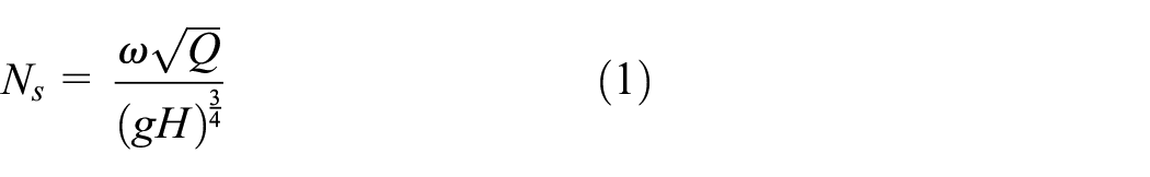
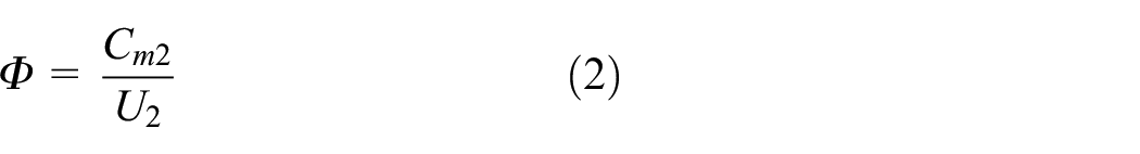
Two mixed-flow pumps with different suction performance are selected for the gradient analysis of head drop. These model pumps were optimally designed using the response surface method (RSM) after applying 2k factorial design so that the design flow rate is near the best efficiency point (BEP).16–18 Table 1 lists the specifications of each model, where subscript 1, h, and s represent the inlet, hub, and shroud, respectively. Type B was designed to have a larger incidence angle and a narrower inlet diameter than type A. Figure 1 shows the meridional plane of the two models. The specific speed (N s ), flow coefficient (Φ), and head coefficient (Ψ) are defined as

Design specification of each mixed-flow pump model.


Meridional plane of each mixed-flow pump model.
where ω, Q, H, g, Cm2, and U2 denote the angular velocity, volumetric flow rate, total head, acceleration due to gravity, meridional component of absolute velocity at the impeller outlet, and rotational speed at the impeller outlet, respectively.
In this article, tip clearance was not considered in the numerical analysis but was considered in the experimental test. Figure 2 shows the results of the experimental test and numerical analysis for types A and B to verify the influence of tip clearance on the performance of a mixed-flow pump. 19 The total efficiency in Figure 2 is non-dimensionalized based on the design point of the numerical analysis results of type B (η des ), which is indicated by the dotted line, and the design flow coefficient is 0.19. Meanwhile, leakage, mechanical loss, and roughness were not considered in the numerical analysis. Furthermore, the experimental setup consists of complex curved pipes along the closed-loop, whereas a straight flow passage was designed for the inlet and outlet for convergence in the numerical analysis. Thus, the results of the numerical analysis exceed the experimental result.20,21 The differences in dimensionless efficiency and head coefficient between the numerical analysis and experimental test at the design flow rate are 0.11 and 0.02 for type A, and 0.11 and 0.05 for type B, respectively. However, the tendency of the curves agrees reasonably well for both results, including the BEP.

Results of numerical analysis and experimental test: (a) type A and (b) type B.
Moreover, the diffuser was not considered in this study to save analysis time. Since the diffuser restores the static pressure of a pump at the rear part of the impeller, the presence or absence of a well-made diffuser has little effect on the tendency of the performance curves or cavitation characteristics of head drop. 22 To confirm the effect of a diffuser on the performance curves in this study, Figure 3 is shown with the numerical results of type B. At the design point, the numerical differences of dimensionless efficiency and head coefficient are 0.04 and 0.03, respectively. Nevertheless, the tendency is almost the same. It can be considered that the diffuser was designed through the optimization process.16–18 Thus, the effects of the diffuser are insignificant. These factors are discussed again for cavitation characteristics in the results part below.

Numerical results of type B for the influence of a diffuser on the performance curves.
Numerical analysis setup
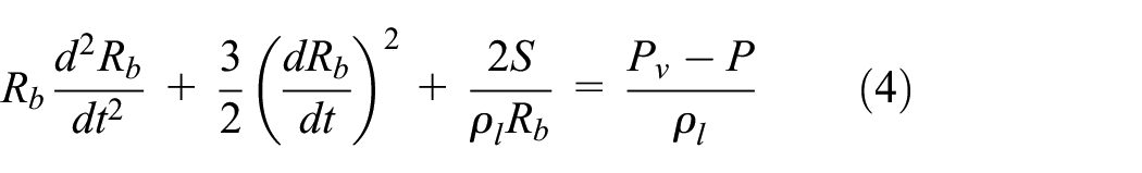
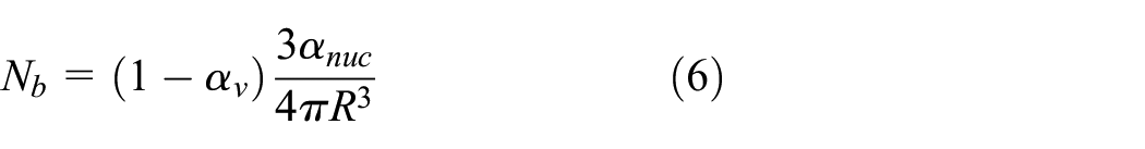
The numerical analysis was performed using ANSYS CFX 16.1. The Reynolds-averaged Navier–Stokes (RANS) equations were discretized using the finite volume method (FVM). A high-resolution discretization of second-order approximation was applied to ensure physical boundaries and numerical convergence, instead of first-order schemes.23,24 The root means square (RMS) residuals of the governing equations and imbalances of mass and momentum were kept below 1.0 × 10⁻⁵ and 1.0 × 10⁻³, respectively, to ensure the required convergence for numerical analysis.25,26 In the unsteady-state analysis, time variation term is added to each governing equation. The shear stress transport (SST) model was applied as a turbulence model to simulate the cavitation phenomenon. 4 For the suitable cavitation model, the Rayleigh–Plesset equation (RPE) was employed to analyze the two-phase transition.12,27–29 For a single bubble in an unbounded incompressible liquid, the Rayleigh–Plesset cavitation model, derived from a momentum balance in the absence of thermal effects, is as follows
where


where

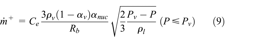

where
A boundary condition of the frozen-rotor method was applied on the interfaces of inlet-impeller and impeller-outlet to transmit data to the next stage without averaging, as only one rotor domain was available for steady-state analysis. The transient rotor-stator method was applied for unsteady-state analysis. For the wall boundary, automatic wall function was applied with smooth and non-slip condition. A periodic condition was applied on single-passage to ensure temporal efficiency, however, full-passage analysis was also conducted to investigate the entire flow field. The atmospheric pressure and mass flow rate conditions were applied to the inlet and outlet, respectively. The working fluid is water and vapor at 25°C. An unsteady condition was applied at every 3° to observe the bubble characteristics based on the time variables of the rotating domain. Seven revolutions of data were obtained for the appropriate convergence. The results were discussed based on the data from the last revolution. The simulations were performed on parallel PCs with Intel Xeon CPU clocked at 3.40 GHz. The computational durations for single-passage of steady-state, single-passage of unsteady-state, and full-passage of unsteady-state were about ∼50 min, ∼3 days, and ∼1 week, respectively.
Grid system
Figure 4 shows a hexahedral grid system generated using ANSYS TurboGrid 16.1. The inlet and outlet of the entire domains are represented for only single-passage, while the impellers are represented for the full-passage. Figure 4(b) shows the impeller LE at the shroud span, marked with a white box in Figure 4(a). Figure 5 shows the distribution of y+ on the impeller surface. Although the low Reynolds number of SST model near the wall recommends a grid system constructed with y+ less than 1, y+ was kept below ∼15 at each surface to satisfy the aspect ratio limit. Moreover, an automatic wall function was adopted so that y+ does not affect the results of the numerical analysis.34,35

Hexahedral grid system for numerical analysis: (a) full scale and (b) enlarged scale.

Distribution of y+ on impeller surface: (a) suction surface and (b) pressure surface.
Figure 6 shows the results of the grid dependency test. Approximately 525,000 nodes do not affect the performance of the pump. Meanwhile, the efficiency shown in Figure 6 is non-dimensionalized based on the maximum value of the grid dependency test (ηmax). All the analyzed sets in this article were considered the same geometric factors as each grid system.

Result of grid dependency test.
Steady-state cavitation
Validation with experimental test
The reliability of the numerical analysis is validated in comparison with experimental results before investigating the cavitation phenomenon based on the suction performance of a mixed-flow pump. Figure 7 shows the closed-loop diagram of the constructed experimental facility. The facility meets the ISO 5198 36 and ANSI/HI 1.6 37 standards. The maximum standard deviation of the measuring instruments such as pressure gauges, temperature sensor, magnetic flow meter, and torque meter is ±0.2%. The flow rate was controlled using two gate-type valves. The pressure in the closed-loop was regulated through the vacuum pump and compressor from the design point.

(a) Schematic diagram and (b) image of the experimental facility.
Experimental tests were conducted for types A and B, and cavitation characteristics for the presence or absence of tip clearance and diffuser were verified once again. Meanwhile, tip clearance was not considered in the numerical analysis, but in the experimental test. To express the cavitation characteristics, cavitation coefficient (σ) and net positive suction head (NPSH) are defined as


where U2, P1, and P v represent the rotational speed at the impeller outlet, inlet total pressure, and saturation vapor pressure, respectively.
Figure 8(a) shows the validation of type A. The result of the numerical analysis only for the impeller is located at the highest position while the numerical analysis result for the impeller and diffuser is located in the middle position. In addition, the experimental test result for the impeller, diffuser, and tip clearance is located at the lowest position. At 0% head drop, each Ψ is 0.55, 0.51, and 0.48 from the top. The tendencies and differences in each Ψ have similar ranges as in Figures 2 and 3, indicating that the total head is reduced due to the inclusion of the diffuser and tip clearance. Moreover, σ at 3% head drop is 0.11, 0.10, and 0.16 from the top, which are relatively similar to each other. Meanwhile, the highest value of σ at 3% head drop is in the experimental test. However, for all three results, a steep head drop occurs near 3% head drop with similar gradients. These results are comparable to the validation results of type B in Figure 8(b). The influence of the diffuser and tip clearance in type B is similar to the coefficient values of type A. Based on 0% head drop, Ψ is 0.58, 0.53, and 0.50 from the top. However, the σ at 3% head drop is 0.78, 0.75, and 0.78 from the top, which is higher than type A. This indicates a poor suction performance. In addition, the head tends to gradually decrease from around σ = 1.9 as the inlet pressure decreases, in comparison with type A.

Validation of numerical analysis with head-drop cavitation characteristics: (a) type A and (b) type B.
From the validation results, the diffuser and tip clearance affect Ψ and σ, which indicate the head rise and suction performance, respectively. However, the cavitation characteristics of the head drop gradient for the two models still differ remarkably even when analyzing the impeller with considering the diffuser and tip clearance. Regardless of the tip clearance and diffuser, type A with a smaller incidence angle has a steep head drop than type B. The cavitation characteristics of the head drop gradient for both types are less affected by the tip clearance and diffuser.
Cavitation phenomenon
Figure 9(a) is expressed as a percentage of the head drop for the two models with respect to the decrease in σ. The head drop gradient is more prominent to compare each model. Type A shows a drastic reduction in the head at 3% head drop (σ = 0.11) while type B shows a gradual decrease to 3% head drop (σ = 0.78). Figure 9(b) shows the efficiency drop for each point in Figure 9(a). Each point is presented as a percentage of the efficiency based on non-cavitation condition. The efficiency of type A is higher than type B in all the points because the head of type A drops more slowly. Meanwhile, the efficiency drops with decreasing the head, but the gradient is slightly different.

Cavitation characteristics for head drop and efficiency drop gradients: (a) head drop and (b) efficiency drop.
In addition, Figures 10 and 11 show the vapor volume fraction at each span (blade-to-blade view) and suction surface (top and 3D view) for types A and B. The observation points are compared at the same σ value, as indicated by the dashed line in Figure 9(a). The vapor volume fraction is expressed from 0 to 1 as the amount of vapor in a cell of the mesh, where 0 indicates that the cell is full of water. For one exception, the vapor volume fraction at 0.1 is presented especially for the 3D view. The figures show that the amount of bubbles increases with decreasing inlet pressure (σ). The bubbles are gradually developed from the impeller shroud LE of the suction surface. Meanwhile, the amount of increasing bubbles due to the decrease in inlet pressure is similar in both models. This can be quantitatively compared with Figure 12, which is the vapor volume in the impeller domain of Figure 4. Actually, more vapors occur in type B at the same σ. However, the vapor amount increases as the inlet pressure decreases with the same tendency of the gradient. This is in contrast to the head drop gradient of Figure 9(a). Therefore, the absolute vapor volume cannot have a significant influence on the suction performance of the pump. The gradient of absolute vapor volume is more similar to the efficiency drop of Figure 9(b).
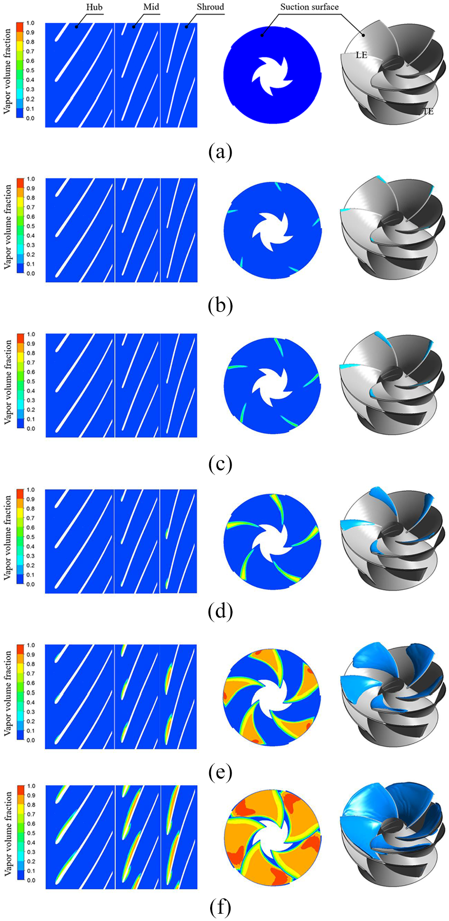
Vapor volume fraction on the impeller suction surface and each span for type A: (a) non-cavitation, (b) σ = 1.20, (c) σ = 0.78, (d) σ = 0.41, (e) σ = 0.19, and (f) σ = 0.11.

Vapor volume fraction on the impeller suction surface and each span for type B: (a) non-cavitation, (b) σ = 1.20, (c) σ = 0.78, (d) σ = 0.41, and (e) σ = 0.19.

Vapor volume in the numerical domain of the impeller: (a) full scale and (b) enlarged scale.
In other words, the head drop gradient for each σ is important. Considering Figure 9(a), the 3% head drop for type B is σ = 0.78. However, the head of type A at the same σ (σ = 0.78) is just beginning to decrease. Besides, the head of type A at σ = 0.19 (shown in Figure 10(e)) does not attain 3% head drop, although it has more vapor amount than 3% head drop for type B (Figure 11(c)). These results are consistent with the quantitative tendency in Figure 12.
The two model types having different suction performance show a clear difference in head drop due to the decrease in inlet pressure. However, it is difficult to determine the cause of this difference with the amount of vapor volume. In addition, Figure 13 shows the vapor volume of type A at σ = 0.78. Although a very small amount of vapor is generated, the head of a mixed-flow pump is affected.
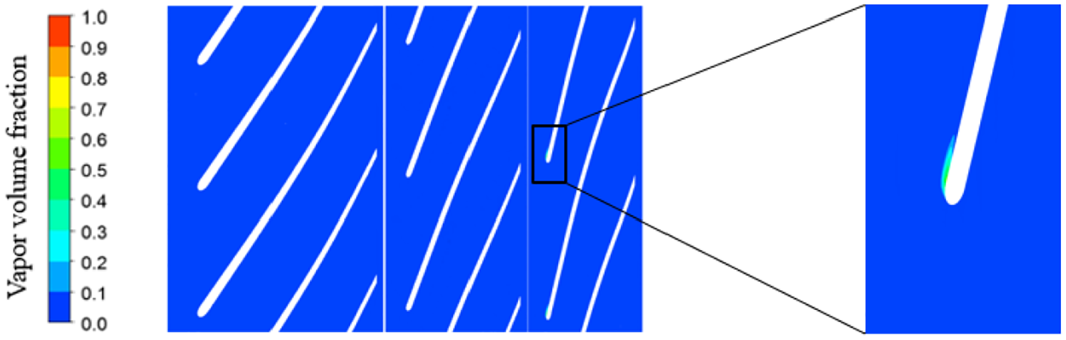
Vapor volume fraction of type A at σ = 0.78.
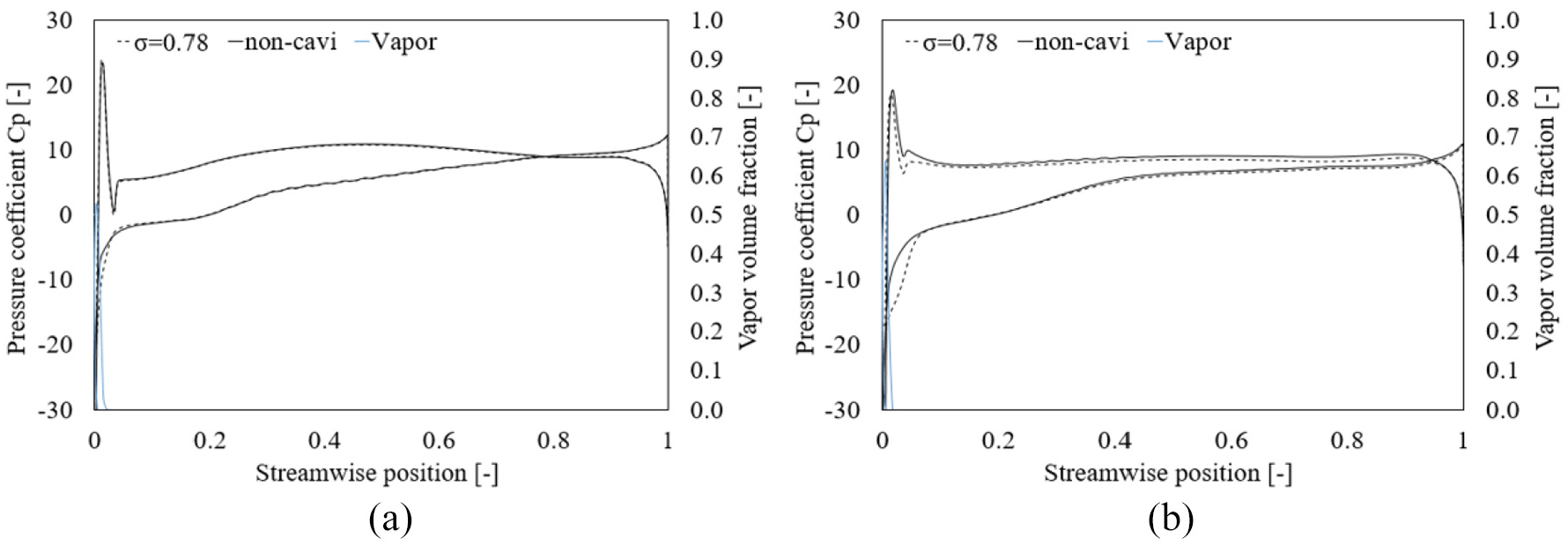
Figures 14 and 15 show the pressure rise along the streamwise position at several points of the same σ, to observe the details of the difference in head drop. The streamwise position is normalized to 0 and 3 for the inlet and outlet of the pump, respectively, and the averaged value of the quasi-orthogonal plane from hub to shroud span is presented. The pressure is non-dimensionalized to the pressure coefficient (C p ) as

where P, P1, and W1 denote the static pressure, inlet total pressure, and relative velocity at the impeller inlet, respectively.

Pressure rise distribution for type A: (a) full scale and (b) enlarged scale.

Pressure rise distribution for type B: (a) full scale and (b) enlarged scale.
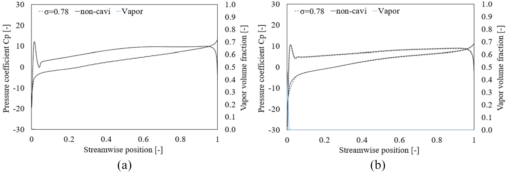
Figure 14(b) shows that the pressure of type A is almost the same in comparison with the non-cavitation state until σ = 0.78. And then, the pressure significantly decreases at the inlet pressure of less than σ = 0.78. However, in Figure 15(b), the pressure decreases gradually as σ decreases. Figure 16 shows the distribution of the minimum C p near the impeller LE with respect to each σ, based on Figures 14 and 15. Type A shows a steep gradient at 3% head drop (σ = 0.11), while type B shows a gradual head drop. The overall tendency is also consistent with Figure 9(a) except for one point of type B where σ is less than 0.78.

Minimum Cp with decreasing σ.
On the contrary, both models exhibit a pressure drop near the impeller LE, which is not recoverable to the outlet as shown in Figures 14 and 15. In both models, obvious pressure drops are observed at the impeller LE. These drops tend to be maintained as it reaches the outlet of a pump. Thus, the pressure drop near the impeller LE determines the pressure rise of the pump. Moreover, bubbles are one of the leading causes of the head drop because bubbles are generated from the impeller LE as the inlet pressure reduces. Furthermore, the two models with different suction performance have different head drop characteristics.
To further clarify the relationship between bubble generation and head drop, the two models are compared at the same inlet pressure at 3% head drop of type B (σ = 0.78). Figures 17–19 show the pressure distribution and vapor volume along the blade surface. The pressure distribution and vapor volume indicate the values from LE to TE (0–1) for the pressure and suction surfaces of the blade, respectively. The figures are enlarged in Figures 20–22 focusing on the LE (0–0.1). First, Figure 19 shows the shroud span, where the largest amount of vapor is generated for each model. Type A has nearly the same distribution between the non-cavitation state and σ = 0.78. However, type B shows a definite difference near the impeller LE. The pressure drops around the impeller LE at σ = 0.78, and is not recovered to the TE. This tendency is observed in all spans of Figures 17 and 18. The deviation between the non-cavitation state and σ = 0.78 is proportional to the amount of generated vapor. At the hub span, there is a very small difference in pressure distribution between the non-cavitation state and σ = 0.78 because no vapor is generated.

Distribution of pressure and vapor volume fraction on the hub span: (a) type A and (b) type B.
Distribution of pressure and vapor volume fraction on the mid span: (a) type A and (b) type B.
Distribution of pressure and vapor volume fraction on the shroud span: (a) type A and (b) type B.

Distribution of pressure and vapor volume fraction on the hub span near LE: (a) type A and (b) type B.

Distribution of pressure and vapor volume fraction on the mid span near LE: (a) type A and (b) type B.

Distribution of pressure and vapor volume fraction on the shroud span near LE: (a) type A and (b) type B.
Thus, type A has no change in pressure despite the occurrence of the vapor at σ = 0.78. Meanwhile, type B shows a significant difference near the impeller LE. It is certain that there is a cause of the head drop near the impeller LE where the vapor is generated.
Another noticeable difference can be confirmed with the vector analysis of the two models. Figure 23 shows the distribution of the flow vector around the impeller LE observed in the shroud span at σ = 0.78 with the vapor volume fraction. The flow rate and rotational speed are the same for both models, so the flow angles cannot be altered. However, type A was designed with a smaller incidence angle than type B, as shown in Table 1. Figure 23 shows that the difference in incidence angle affects the vector distribution of the flow, especially on the suction surface. The flow vector is consistent with the blade surface in type A. However, type B has a larger vector component in the circumferential direction immediately after the stagnation point. Moreover, it has a wider range of reattached flow near the LE of the suction surface where the vapor begins to occur.

Distribution of the flow vector around the impeller LE on the shroud span (σ = 0.78): (a) type A and (b) type B.
The circumferential water velocity near the LE is extracted and shown in Figure 24. Figure 25 shows the definition of the planes in Figure 24. The streamwise position from the LE to the TE of each span is normalized to 0 and 1, respectively, and the planes are expressed as a percentage. The circumferential velocity component of type B is larger than type A and gradually decreases from the LE to the flow direction. Meanwhile, the vapors begin to form near the suction surface of the impeller LE, as shown in Figure 13. In other words, type B has a larger circumferential velocity component near the suction surface of the impeller LE, which can affect the shape of the vapor.

Circumferential component of water velocity near the LE (σ = 0.78): (a) 0.0% (LE), (b) 0.2%, (c) 0.4%, (d) 0.6%, and (e) 0.8%.

Explanation for defined planes in Figure 24.
From the results above, the pressure drop near the impeller LE caused by the generated vapor is directly related to the head performance of the mixed-flow pumps. Moreover, the level of the pressure drop near the impeller LE is significantly different for the two models with different incidence angles. The difference in the incidence angle has a significant influence on the internal flow at the suction surface of the impeller LE, where the vapor is mainly distributed. On the contrary, the amount of vapor increases with decreasing inlet pressure. However, it is impossible to account for the 3% head drop point with the vapor amount.
Unsteady-state cavitation
Single-passage analysis
Focused on the differences in vector components due to the incidence angles, Figure 26 is shown to observe the shape and patterns of vapor with time variation. Numerical analysis was performed for the domain corresponding to the single flow passage. The result shows the averaged vapor volume from hub to shroud span. The vapor volume fraction on the x-axis is also expressed from 0–1, but is enlarged from 0–0.3. Meanwhile, a small amount of vapor volume is distributed at σ = 0.78, especially near the shroud span. However, these bubbles cause the 3% head drop of type B.
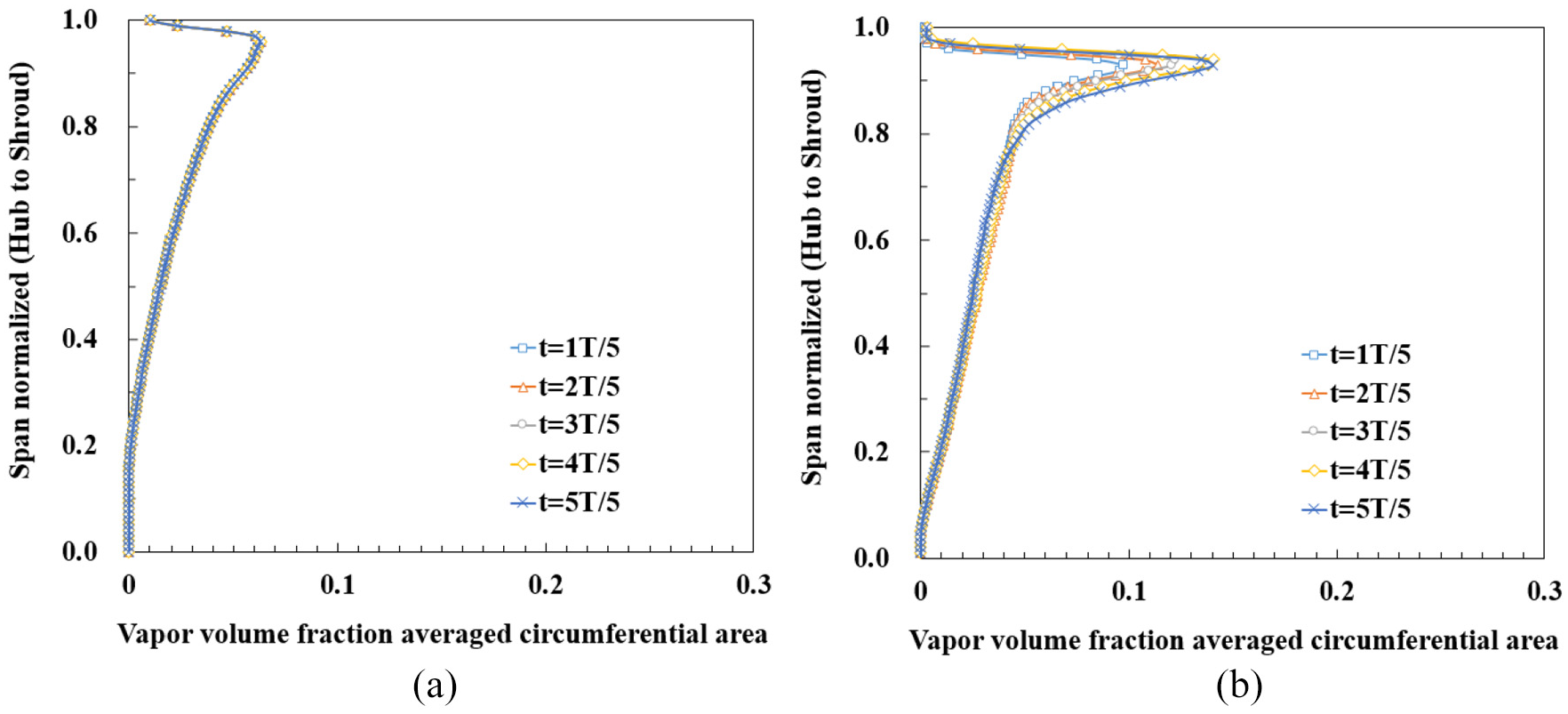
Vapor volume fraction averaged circumferential area on the impeller LE (σ = 0.78): (a) type A and (b) type B.
Figure 26(a) shows the vapor volume fraction of type A. Although the impeller rotates, the amount and shape of the bubble remain unchanged with time variation. Figure 26(b) shows that the generated bubbles are relatively unstable as their pattern with time variation. This phenomenon can be severe to internal flow during pump operation because the bubble displaces liquid due to the cross-sectional blockage. 38 The bubbles inside the pump interfere with the internal flow and act as additional blockage. 14
This irregular pattern of bubbles can be applied to investigate the reason for the difference in the gradient of the head drop. That is, the mixed-flow pump for type B with a relatively irregular pattern of generated bubbles is found to exhibit a faster head drop than type A. In other words, the head of type A with a suitable incidence angle lasts longer in the non-cavitation state with decreasing inlet pressure. The instability of the vapor pattern can be directly related to the circumferential velocity component caused by the incidence angle.
In addition, Figure 27 shows the effect of the incidence angle on the stability and pattern of the bubble more clearly. The 3% head drop for type A occurs at σ = 0.11 with a significant amount of generated bubbles, as shown in Figure 10(f). However, a constant vapor distribution is obtained with time variation. Thus, the difference in the incidence angle determines the stability of the vapor distribution.

Vapor volume fraction averaged circumferential area on the impeller LE for type A (σ = 0.11).
Full-passage analysis
Types A and B have five blades each. Numerical analysis of the full-passage was performed to observe the variation of the bubble in each blade with time variation. Prior to that, the influence of the periodic conditions on the cavitation characteristics of the head drop was verified to compare both the models. The results of the cavitation analysis for the full-passage are shown in Figure 28. The experimental results and the CFD results of single-passage analysis in Figure 28 are the same as the results in Figure 8. Each result of the single-passage, full-passage, and experimental results show an excellent agreement in the head drop gradient of the cavitation characteristic.

Validation of cavitation analysis for full flow passage: (a) type A and (b) type B.
Figure 29 shows the pattern of the generated bubbles along the shroud span of the LE as defined in Figure 30. As each model has five blades, the peak point of vapor volume fraction is observed at every 72°. In Figure 29(a), the bubbles distributed on each blade of type A show an almost constant pattern with a slight deviation. However, it is difficult to observe any pattern in the vapors distributed on each blade of type B in Figure 29(b). The value of the vapor volume fraction on each blade for type B is more irregular than type A. As the impeller rotates, the amount of generated bubbles changes from time to time.

Generated bubble patterns on the LE of shroud span for each blade (σ = 0.78): (a) type A and (b) type B.

Designated line for the extracted data in Figure 29.
As a citation in some previous studies, these oscillations of bubbles can have a profound effect on the pressure fluctuations during pump operation.39,40 From their results, the amplitude and magnitude of pressure fluctuations are sensitively affected by changes of the bubbles. The unsteady condition such as broad-band pressure fluctuation is proportional to the degree of cavitation and vapor volume fraction. The pressure fluctuations inside the pump is a detrimental component that degrades the performance of the pump and increases vibration and noise at the same time. Hence, the shape and pattern of the generated bubble lead to a difference in the suction performance owing to the gradient of the head drop. Although the amount of vapor inside the pump is quite small, its stability of the vapor is analyzed to affect the head of the pump. 41
In addition, Figure 31 verifies the above cavitation characteristics for the patterns of the generated bubble on the LE of shroud span with each blade of type A at σ = 0.11. Each blade has a regular distribution, although the amount of vapor is larger than σ = 0.78. Thus, the correlation between the amount and stability of the generated vapor can be neglected. This is because the incidence angle of type A is relatively smaller than type B. Type A has a stable vector distribution on the suction surface of the impeller LE in comparison with type B. Therefore, the incidence angle is one of the most important design variables to determine the cavitation performance of a mixed-flow pump.

Generated bubble patterns on the LE of shroud span for each blade of type A (σ = 0.11).
Conclusion
In this article, the shape and pattern of a bubble were analyzed for two models with different suction performances. The cause of the head drop gradient was presented with steady- and unsteady-state analyses. The head drop gradient was confirmed based on suction performance. The differences in each model were discussed from various viewpoints. Moreover, the numerical analysis was validated with the experimental test. The results can be summarized as follows:
Bubbles are generated from the suction surface of the impeller LE as the inlet pressure decreases, and the amount increases gradually. However, the amount of bubbles cannot determine the suction performance of a pump.
The incidence angle has a proportional effect on the circumferential velocity component of a pump, especially near the shroud. The region where the circumferential velocity component is mainly distributed is almost the same as the position where the bubble is generated under cavitation.
From the results of the unsteady Reynolds-averaged Navier–Stokes (URANS) simulation, a pump with relatively good suction performance (type A) exhibits a uniform vapor distribution even when the impeller rotates. A pump with poor suction performance (type B) obtains non-uniform vapors for each blade. The differences in incidence angles can affect the shape and pattern of the generated bubbles.
If the generated bubbles do not have a uniform pattern, the head drop occurs faster. The shape and pattern of the vapor are closely related to suction performance. Hence, these cavitation characteristics can be useful factors in determining the suction performance of a mixed-flow pump.
Footnotes
Appendix
Handling Editor: James Baldwin
Declaration of conflicting interests
The author(s) declared no potential conflicts of interest with respect to the research, authorship, and/or publication of this article.
Funding
The author(s) disclosed receipt of the following financial support for the research, authorship, and/or publication of this article: This work was supported by the Development of Design Technology for Thermal Energy Devices with Industrial Demand (grant no. KITECH JA-19-0011) from the Korea Institute of Industrial Technology (KITECH).