Sage Journals: Discover world-class research

Abstract

Computational fluid dynamics is an essential tool for the flow field analysis of the blood pump. The interface processing method between the dynamic/static regions will affect the accuracy of simulation results, but its influence on the simulation results is still unclear. In this study, the axial-flow blood pump was taken as the research object, and the effects of the mixing plane, frozen rotor, and sliding mesh methods on the following results were compared: flux conservation at the interface, hydraulic characteristics, and velocity field distribution. In parallel, the particle image velocimetry experiment was carried out to measure the velocity field of the impeller, the inlet, and the outlet area of the blood pump. The results show that the above methods have significant differences in flux conservation between the impeller and the back vane. The average surface energy flux’s error of frozen rotor and sliding mesh are 0.7% and 0.72%, respectively, while the mixing plane method reaches 3.6%. This nonconservative transfer affects the distribution of the downstream velocity field, and the velocity field predicted by the mixing plane at the outlet is quite different. It is suggested to use the frozen rotor method and the sliding mesh method in the simulation of the blood pump.

Keywords

Blood pump computational fluid dynamics rotor stator interface processing

Introduction

There are currently more than 20 million heart failure patients worldwide,¹ and the incidence is rising rapidly due to the aging population.² Supporting the natural heart by implanting a blood pump has become the optimal treatment option in the absence of a cardiac donor, rotary blood pumps are widely used in clinical assistance, and the axial-flow blood pump is one of the main forms.^3–6 However, an unreasonable design of the blood pump structure will cause instability in the internal flow field, which will lead to hemolysis and thrombosis. This problem is considered to be one of the factors restricting the long-term application of a blood pump in the body.^7–10 Since computational fluid dynamics (CFD) can simulate the complex flow state of fluid and realize the visualization of the flow field, CFD has been widely used in flow field analysis and structural optimization of blood pumps to solve these problems.^11–14

Blood is mixed with a large number of red blood cells and white blood cells. At present, there are some models¹⁵ and methods^16–18 that can analyze the interaction between particles and fluid from a microperspective. However, the number of red blood cells (millions) in the blood pump is a challenge to the computer hardware. Therefore, the single-phase flow method is often used in CFD simulation research of blood pumps.¹⁹ While relevant settings in CFD will directly affect the accuracy of simulation results, different researchers have different settings in blood pump simulation research. In the case of a specific grid and right boundary conditions, the selection of the turbulence model and the processing method of the dynamic/static interface are the main factors affecting the results. Researchers compared the effects of turbulence models on blood pump simulation results, which show that the shear stress transport (SST) k-ω model is suitable for the simulation of the blood pump.^20–22 However, in the research of the dynamic/static interface processing method, the existing research mainly focuses on other types of fluid machinery. J Karnahl et al.²³ studied the effects of different dynamic/static interface treatments on flow and heat transfer in a preswirl system, and the result shows high variability in pressure and velocity distributions at the preswirl inlet nozzle radius. M Beaudoin et al.²⁴ proposed an improved mixing plane model based on the OpenFOAM and compared it with the traditional mixing plane method. The results show that the interface processing method will directly affect the data transmission between the static and dynamic regions, and thus affect the simulation results. Shim and Kim²⁵ took centrifugal pump as the research object and analyzed the influence of the interface treatment method on the simulation results of hydraulic performance, but did not verify the results of the velocity field. Although the interface methods were discussed in the above studies, the structure of the research object is different from that of the blood pump. Furthermore, the flow field was not verified by experiments, so the results may not be suitable for the blood pump. Currently, there are different dynamic/static interface processing methods in blood pump simulation research, such as the mixing plane method,²⁶ the frozen rotor method,²⁷ and the sliding mesh method;¹⁴ however, there is a lack of comparative study between the above methods, and its impact on the simulation results is not clear. The particle image velocimetry (PIV) experiment is an important method to verify the simulation results of flow field.^28,29 However, due to the occlusion of the internal structure by the blood pump driving system, there are few PIV experiments for the internal velocity field of the blood pump.^30,31

In summary, the influence of which interface processing method on the CFD simulation results of the blood pump is still unclear. In the existing research works, the researchers used different interface processing methods in simulation, and the simulation results may mislead the investigation. Furthermore, due to the limitation of the axial-flow blood pump’s driving system, the internal velocity field is difficult to be photographed, which aggravates the difficulty of experimental verification. In this article, the axial-flow blood pump is taken as the research object. Different from the previous research, a novel driving system for the axial-flow blood pump was designed to overcome the limitations imposed by the traditional drive structure, and the PIV experiment of the internal flow field of the blood pump was carried out. The conventional dynamic/static interface processing methods (the mixing plane, frozen rotor, and sliding mesh methods) in blood pump simulation were compared. Through the PIV and hydraulic performance tests, simulation results of the pressure–flow characteristic and the velocity filed were verified. Through this study, it can provide a reference for the interface setting of the simulation of the axial-flow blood pump, and reduce the result interference caused by improper interface setting.

Interface processing method theory

Mixing plane method

The mixing plane method divides the computational domain into a rotating domain and a static domain, the plane where the domains intersect is called a hybrid plane. The mixing plane method treats each solution region as a steady-state problem. In the rotating domain, the flow control equation is solved in a rotating coordinate system. In the static domain, the flow control equation is solved in a stationary coordinate system. In order to realize the data transfer between regions, the mixing plane method constructs the inlet and outlet boundary conditions at the interface, and the data are transmitted to the downstream region in a circumferential or radial average. At present, there are three main average methods used, namely, the area average method, the mass average method, and the mixed average method. When using the boundary conditions of the pressure inlet and the mass flow outlet, Fluent adopts the mass average method, and the average formula is shown as in equation (1)

m = \int_{A} ρ V n dA

(1)

where A is the area of the interface, m is the mass flow rate of the flow area, n is the unit normal vector, V is the volume, and ρ is the density.

Frozen rotor method

Similar to the mixing plane method, the frozen rotor method also divides the computational domain into a rotating domain and a static domain. The relative position between the rotating domain and the static domain is constant, and the fluid equations are solved in the rotating coordinate system and the stable coordinate system, respectively. It is an approximate steady-state processing method. The main difference between it and the mixing plane is that the frozen rotor method passes the data at the interface by interpolation. The freezing factor uses the interpolation method when transferring data at the interface. The processing method of the velocity vector is shown in equation (2)

v = v_{r} + v_{t} + ω \times r

(2)

where v is the absolute velocity (the velocity observed from the stationary frame), v_r is the velocity of the moving frame relative to the inertial reference frame, v_t is the translational frame velocity, ω is the angular velocity, and r is the vector pointing to the center of rotation. The velocity and the velocity gradient are converted from the driven coordinate system to the absolute inertial coordinate system, and then the absolute velocity vector can be obtained. Scalar information such as temperature, pressure, and density can be obtained from the adjacent grid cells and interpolated.

Sliding mesh method

The sliding mesh processing method has many similarities with the freeze factor method. Both of them divide the domain into a rotating domain and a static domain, and the data transmission at the interface is also processed by interpolation. The characteristic of the sliding mesh is that the relative position between the stator and the rotor in the sliding mesh changes with time, and the dynamic update of the grid adopts the processing method of the moving grid, but the deformation amount of the grid is zero. It has the characteristics of describing the time-varying features of the interface. The movement of its boundary is defined by equation (3)

\frac{d}{dt} \int_{V} ρ ϕ dV = \frac{{(ρ ϕ V)}^{n + 1} - {(ρ ϕ V)}^{n}}{Δ t}

(3)

where V is the control volume; ρ is the fluid density; n and n + 1 denote the respective quantity at the current and the next time levels, respectively; and $ϕ$ is the general scalar on an arbitrary control volume.

Model and simulation setup

Blood pump model

As shown in Figure 1, the axial-flow blood pump used in the experiment and simulation was developed by the Central South University. The length and the diameter of the blood pump are 73 and 16.5 mm, respectively. According to the demand of normal blood flow of the human body, its rated flow rate is 5 L/min, the pressure difference is 13.3 kPa, and the rated speed is 8000 r/min. The blood pump is composed of a front vane, an impeller, and a back vane. The impeller has a permanent magnet inside, and the impeller rotates by the external magnetic field to transport blood from the inlet to the outlet. The interface between the impeller region and the front vane region is the dynamic/static interface 1, and the interface between the impeller region and the rear vane region is the dynamic/static interface 2.

Figure 1.

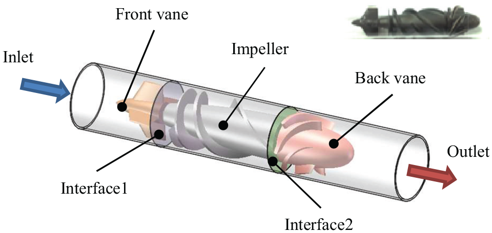
Blood pump model.

Selection of turbulence model

This simulation is based on the Fluent 17.0 software (ANSYS, Inc., Canonsburg, PA, USA), which uses the finite volume method to solve the Navier–Stokes (N-S) equations. In this simulation, the fluid is assumed to be incompressible. In the choice of turbulence model, since the SST k-ω model contains the modified turbulent viscosity formulas and considers the effect of turbulent shear stress, it can simulate the near-wall flow field more accurately and proved to be suitable for blood pump simulation.^20–22

The expression of SST k-ω model³² is shown in equations (4) and (5)

\begin{matrix} \frac{\partial}{\partial t} (ρ k) & + \frac{\partial}{\partial x_{i}} (ρ k u_{i}) = \frac{\partial}{\partial x_{j}} ((μ + \frac{μ_{t}}{σ_{k}}) \frac{\partial k}{\partial x_{j}}) \\ - ρ \bar{{u'}_{i} {u'}_{j}} - ρ β^{*} k ω \end{matrix}

(4)

\begin{matrix} \frac{\partial}{\partial t} (ρ w) & + \frac{\partial}{\partial x_{i}} (ρ w u_{i}) = \frac{\partial}{\partial x_{j}} ((μ + \frac{μ_{t}}{σ_{ω}}) \frac{\partial w}{\partial x_{j}}) \\ - α ρ \bar{{u'}_{i} {u'}_{j}} \frac{ω}{k} - ρ β ω^{2} \\ + 2 (1 - F_{1}) ρ \frac{1}{σ_{ω 2} ω} \frac{\partial k}{\partial x_{j}} \frac{\partial ω}{\partial x_{j}} \end{matrix}

(5)

where ρ is the fluid density, which is set as 1.07 kg/m³; k is the turbulent kinetic energy; ω is the specific dissipation rate; μ is the dynamic viscosity; μ_t is the turbulent eddy viscosity; F₁ is the blending function, which is used to blend the k-ω model (F₁ = 0) and k-ε model (F₁ = 1); and the model coefficients are as follows: β = 0.075, β^* = 0.09, σ_k = 2, σ_ω = 2, and σ_ω₂ = 1/0.856.

Meshing

In the meshing, to reduce the influence of the inlet and outlet boundary on the result, a certain length of the pipe segment is added to the front and rear guide vanes. The blood pump model grid was created based on ICEM CFD. It was divided by the unstructured tetrahedral mesh, which has good adaptability to complex geometric shapes. After verifying the number of grids, the total number of grids was determined to be 4.5 million. For the SST k-ω model, the requirement for Y+ is less than 1, and the number of boundary layers should be greater than 15. Therefore, the model boundary layer mesh was divided based on the above requirements. The growth factor was set to 1.05, the total boundary layer was set to 20, and the Y+ value was approximately 1. The mesh is shown in Figure 2.

Figure 2.

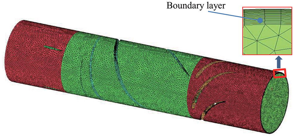
Mesh of the blood pump model.

Interface processing method settings and solver settings

The dynamic/static interface involved in the model is shown in Figure 1. It includes interface 1 between the leading vane area and the impeller area, and interface 2 between the impeller area and the rear guide vane area. In the simulation, mixing plane, frozen rotor, and sliding mesh methods were used for comparison.

The inlet boundary condition was set to the total pressure inlet, the outlet boundary condition was set to the flow outlet (5 L/min), and the blood pump rotation speed was set to 8000 r/min. A second-order upwind advection scheme was set in all cases, with double precision. For time discretization, a second-order backward Euler transient scheme was used. The residual target was set to 10⁻⁵.

PIV experimental system

Design of blood pump external magnetic drive for PIV experiment

At present, most axial-flow blood pumps are driven similarly to brushless motors (Figure 3(a)), that is, the drive coil is wrapped around the outside of the impeller to drive the permanent magnet inside the impeller to rotate.³³ This type of drive occludes the shooting of the flow field in the impeller region. Therefore, there are few PIV experiments on the impeller region of the axial-flow blood pump. To solve the problems, we developed a new blood pump drive system that can effectively drive the blood pump and avoid the occlusion of the internal flow field. The newly designed drive system is shown in Figure 3(b). The motor drives the permanent magnet to rotate on one side of the blood pump. Due to the coupling of the magnetic field, the blood pump rotates synchronously according to the magnetic pole order. The rotary encoder installed on the motor monitors the rotation angle of the blood pump and outputs the PIV synchronized shooting signal.

Figure 3.

Schematic diagram of the axial-flow blood pump’s driving system: (a) traditional drive system and (b) newly designed drive system.

Composition of PIV experimental system

The composition of the test system is shown in Figure 4. The blood pump was installed in a transparent pipe, while a square sink was installed on the outside to minimize the effects of refraction. The laser head was mounted above the blood pump, and the irradiated laser coincided with the central axis of the blood pump. The camera shot the blood pump’s flow field from the direction perpendicular to the laser illumination. Pressure sensors were installed at the inlet and the outlet of the blood pump to measure the differential pressure. The ultrasonic flowmeter was installed in the circulation loop to measure the flow rate. The damping valve was used to adjust the damping of the circuit. The constant temperature water tank was used to ensure that the temperature of the circulation loop is approximately constant.

Figure 4.

PIV test bench composition.

PIV system hardware components

The PIV experimental device adopts the LaVision PIV system. The main components are as follows: the laser adopts the Litron LDY300, and the maximum working frequency is 90 Hz; the PIV camera model is the LaVision ImagerProSX 5M dual shutter camera with a resolution of 2448 pixels × 2050 pixels and a single pixel size of 3.45 μm × 3.45 μm, the minimum cross-frame time is 44 μs, and the maximum frame rate is 14.2 fps. The synchronous shooting system includes LaVision 1108090 synchronizer, rotary encoder, signal transmission cable, and the DaVis processing software.

Solution and PIV tracer particle

In order to simulate the fluid properties of blood, the experimental solution was selected from a 27.3% aqueous glycerol solution with a density of 1.07 kg/m³, and its viscosity index was similar to that of blood. In order to ensure that the seeding particles have good followability and light scattering when moving in the flow field, hollow glass beads with a diameter of 10 μm were selected.

PIV shooting position and calibration

The PIV photographing section is shown in Figure 5. The processed positions are domain 1, domain 2, and domain 3, which correspond to the blood pump inlet, the impeller outlet, and the blood pump outlet, respectively. The reason for selecting domain 2 is because it is the outlet of the impeller, where the fluid is entirely subjected to the rotation of the impeller, and its turbulence develops more fully. The calibration process of PIV is as follows: first, insert a calibration plate (had the same diameter as the pipeline) in the direction of the pipeline axis, then select the marker points on the calibration plate in the DaVis processing software, and calibrate the image size and tilt, and finally, move the calibration plate out of the pipeline after calibration.

Figure 5.

PIV measurement position and calibration.

Flux calculation at the interface

Flux represents the information of mass, momentum, and energy flowing through a normal unit area in a unit time. Flux conservation is one of the important conditions in the finite element volume calculation method. Conservation of flux transfer between dynamic and static interfaces will have an impact on the results. The flux error E (equation (9)) in the upstream and the downstream of the interface is selected to analyze the conservation situation. The flux chosen is as follows: Q_m is the mass flux, Q_vx is the axial momentum flux, Q_vr is the radial momentum flux, Q_vθ is the circumferential momentum flux, and Q_E is the energy flux (equations (6)–(8)), in which v represents the absolute velocity vector, s represents the mesh vector, ρ represents the fluid density, vx represents the axial velocity, vr represents the radial velocity, vθ represents the circumferential velocity, e represents the internal energy of the fluid, Q_up represents the flux through the upstream, and Q_down represents the flux through the downstream.

As shown in Figure 6, the perpendicular planes 1 and 2 are established, and their intersections with interface 1 and interface 2 are line 1, line 2, line 3, and line 4, respectively. The flux conservation of interface 1, interface 2, and line 1 to line 4 is analyzed

Q_{m} = ρ (v \cdot s)

(6)

Q_{vx, vr, v θ} = ρ v_{vx, vr, v θ} (v \cdot s)

(7)

Q_{E} = ρ (e + v^{2} / 2) (v \cdot s)

(8)

E = | \frac{Q_{down} - Q_{up}}{Q_{up}} |

(9)

Figure 6.

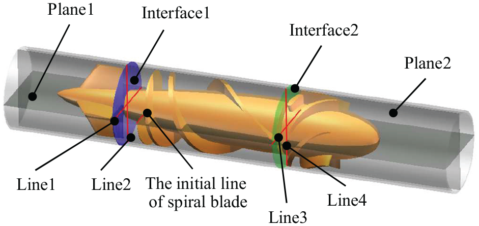
Position for flux conservation analysis.

Results

Flux conservation results

Mean surface conservation results of flux at interface 1 and interface 2

The results of the flux conservation error rate are shown in Figure 7. The maximum mass flux error rate obtained by different interface processing methods is 0.86%. At the interface 1, the axial, circumferential, and radial’s error rates of flux momentum conservation of frozen rotor and sliding mesh are less than 0.5%. The axial, radial, and circumferential momentum flux conservation errors of the mixing plane method are 1.75%, 1.58%, and 2.34%, respectively. At the interface 2, the maximum momentum conservation error rates of the frozen rotor and the sliding mesh are 0.78%, while the axial, radial, and circumferential momentum conservation error rates of mixing plane are 5.9%, 3.25%, and 4.21%, respectively. For the error rate of energy flux conservation, the maximum error rate of the various processing methods at interface 1 is less than 0.8%, and the error of frozen rotor and sliding mesh at interface 2 (maximum 0.72%) is smaller than the mixing plane treatment method (3.72%).

Figure 7.

Surface mean conservation results of flux at interface 1 and interface 2.

Conservation of energy flux at the interface in the circumferential direction

The conservation of the line 1/2/3/4 is analyzed to obtain the conservation variation of the interface in the circumferential direction, and the energy flux—including the sum of hydrostatic pressure and dynamic pressure—is selected for analysis. The result is shown in Figure 8. The abscissa indicates the ratio between the distance r of the point on the straight line from the center of the circle and the radius R of the section circle, and positive and negative indicate the two directions from the center of the circle. As shown in Figure 8(a), the energy flux conservation errors’ variation trend of line 1 and line 2 at interface 1 is similar. The mixing plane has a 40% error at r/R = ± 0.375, and a conservation error of 123% occurs at the near-wall surface. The maximum error of frozen rotor and sliding mesh appears near the wall with the maximum error rate of 18.4% and 13.6%, and the error rate for the rest of the region is close to zero. In the result of interface 2, the energy conservation rate of various treatment methods is close to 0 in the range of r/R from −0.5 to 0.5. The mixing plane method has large fluctuations in the range of −0.75 to −1 and 0.75 to 1, and the maximum error is about 200%. The maximum error of the frozen rotor and the sliding mesh is about 55% and 58%, and the range of error fluctuation is small.

Figure 8.

Energy conservation results in the circumferential direction of the interface: (a) interface 1 and (b) interface 2.

Total pressure distribution at the interface

The total pressure of the system represents the sum of dynamic pressure and static pressure, which can reflect the energy transfer and the distribution in the flow field. The total pressure distribution at the interface is shown in Figure 9, respectively.

Figure 9.

The total pressure distribution at the interface (frozen rotor, mixing plane, sliding mesh, in turn): (a) interface 1 and (b) interface 2.

As can be seen from Figure 9, the total pressure distribution at the interface 1 is uniform because the fluid flow here is a smooth pipe flow. There is almost no difference in various treatment methods. At the interface 2, a larger gradient appears in the total pressure distribution, which is caused by the turbulence generated by the impeller acceleration, and the results have obvious differences. The total pressure distribution of the mixing plane method shows a state of uniform distribution in the circumferential direction, while the frozen rotor and the sliding mesh retain the circumferential nonuniform state of the total pressure of the flow field, which can reflect the influence of static and dynamic interference.

Effect on the result of differential pressure

The rated working condition of 8000 r/min is selected as the simulation and the experiment condition, the pipe resistance is changed, and the change of flow rate and the pressure difference between inlet and outlet is analyzed. The result is shown in Figure 10.

Figure 10.

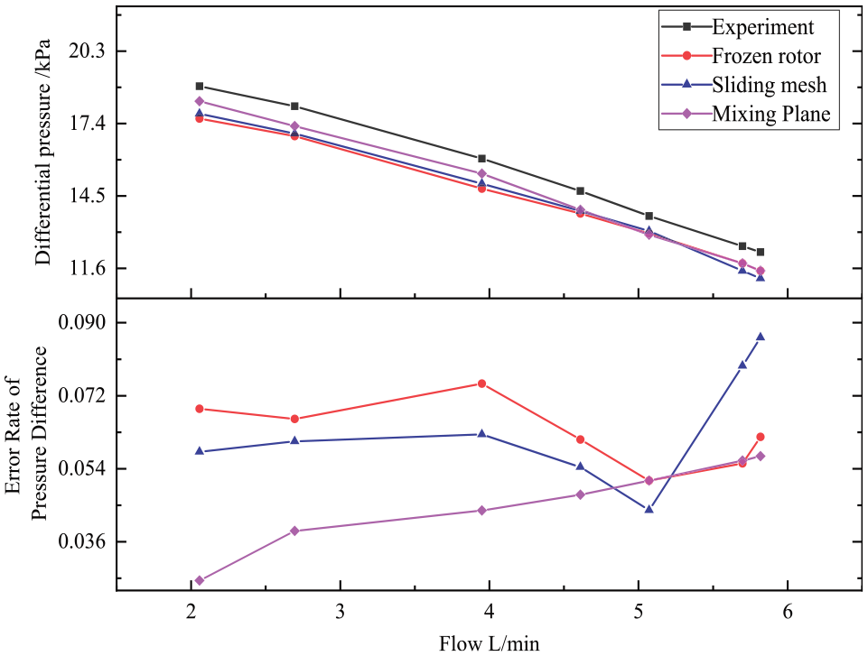
Experimental and simulation results of hydraulic characteristics of the blood pump.

In Figure 10, it can be seen that the simulation results of pressure difference under various interface treatment methods are smaller than the experimental values, the pressure difference decreases with the increase in the flow, and the changing trend is consistent with the experiment. Their prediction errors are about 5% at the operating design point (5 L/min and 13.3 kPa). There is little difference between the prediction results of various interface treatment methods for hydraulic characteristics. In the range deviating from the operating design point, the predicted pressure difference between the frozen rotor and the sliding mesh is smaller than the mixing plane method.

Effect on the velocity field

The same position as the PIV shooting area is extracted from the velocity field simulation result. The velocity vector graphs and contour of the inlet, the impeller, and the outlet area are shown in Figures 11 –13. The color in the figures indicates the velocity value, and the vector indicates the velocity direction.

Figure 11.

Blood pump inlet area (domain 1) velocity field results: (a) PIV experiment result, (b) frozen rotor, (c) mixing plane, and (d) sliding mesh.

Figure 12.

Flow field results of the blood pump impeller (domain 2): (a) PIV experiment result, (b) frozen rotor, (c) mixing plane, and (d) sliding mesh.

Figure 13.

Flow field results in the blood pump outlet area (domain 3): (a) PIV experiment result, (b) frozen rotor, (c) mixing plane, and (d) sliding mesh.

As can be seen in Figure 11, the velocity in the import section is about 0.5 m/s, and the experimental results are in good agreement with the simulation results. The velocity distribution in the inlet domain is relatively average; the velocity near the wall is small due to the viscous boundary layer. The streamline results show that the flow direction of the fluid in this area is parallel to the pipeline axis, which is a stable pipeline flow. The effects of various interface treatment methods are not significant. The velocity and the streamlines obtained by simulation results are basically in agreement with the simulation results.

In Figure 12, it can be seen that the maximum speed in this area is approximately 2.4 m/s, and there are two high-speed zones and one vortex in the flow field of the impeller exit region. The reason for the vortex is as follows: when the fluid flows through the impeller to the rear guide vane, the twisted blade on the rear guide structure has a certain blocking effect on the part of the fluid, so there is a phenomenon of flow separation and vortex, and these areas are potential for blood damage. The above phenomena can be observed through the simulation results of various interface processing methods, and the simulation results can be well matched with the PIV experimental results.

The results of Figure 13 show that the flow velocity at the outlet decreases after flowing through the impeller, and its flow direction is approximately parallel to the pipeline under the correction of the rear guide vane. The results also show that there is a big difference between the simulation results of the mixing plane and PIV experiment results. The PIV experiment results show that the streamline in the exit area is parallel to the axis under the correction of the rear guide vane, and there are two high-speed zones with a maximum velocity of about 0.8 m/s in the near-wall area on the left side. The distribution results of the streamline and high-speed region obtained by the frozen rotor and the sliding mesh are consistent with the experiment, but the velocity distribution in the latter part region is smaller than the experimental result. The simulation results of the mixing plane method show that the velocity field is approximately uniformly distributed in the circumference. The velocity increases with the distance from the axis, and there are large vortices in the center flow field, which is not consistent with the PIV experimental results.

Discussion

During the process of passing through the interface 1, the fluid has not been rotated by the impeller, and its flow state is relatively stable, so the flux of various interface treatment methods can basically ensure conservation. According to the simulation results, after the fluid passes through interface 1, the total pressure rises sharply due to the rotation of the impeller. In Figure 9, it can be seen that there is a significant pressure gradient at the interface 2. At this time, the treatment mode of the interface will have a considerable influence on the results. From the contour of total pressure, we can see the difference in data processing of several methods. Since the frozen rotor and the sliding mesh adopt the interpolation transfer method, the unsteady effect is fully considered in the data transfer, so the flux conservation in the upstream and the downstream of the interface is better, and the total pressure is unevenly distributed in the circumferential direction. However, the mixing plane method uses the averaging process to treat the unsteady flow as uniform flow, which ignores the interference between the static and the dynamic regions. The circumferential total pressure distribution changes uniformly, resulting in significant conservation errors at the interface 2. This is consistent with J Karnahl et al.’s²³ conclusions about the effects of different interface methods on the preswirl system.

Besides, it should be noted that the changing trend of total pressure at interface 1 and interface 2 is different: the total pressure at the interface 1 is the smallest near the wall, because it is a stable pipeline flow, and the velocity near the wall is lower under the action of the viscous boundary layer, so the total pressure is smaller here. However, the total pressure at the interface 2 is higher near the wall, which is due to the thrust and the centrifugal force of the impeller when the fluid flows through the area. This further exacerbates the imbalance of the total pressure distribution in the circumferential direction. Figure 8 shows the conservation of the total pressure in the circumferential direction. Figure 8(a) shows that, in the case where the interface 1 has a small total pressure gradient, the various methods can substantially guarantee the conservation of the total pressure in the circumferential direction. However, the error rate obtained by the mixing plane method is 123%. The main reason for the considerable error may be that the fluid velocity at the viscous boundary layer is minimal, and then a large velocity and a total pressure gradient are generated. However, the thickness of the viscous layer is minimal, so it can be considered that the effect of nonconservation here is small. When the interface 2 is processed by the mixing plane method, Figure 8(b) shows that the regions with high error rates are located at −0.75 to −1 and 0.75 to 1 of r/R, and the maximum error rate of total pressure conservation is over 200%. Figure 9 shows that the pressure gradient in the region as mentioned above is large, and the total pressure distribution in the region becomes uniform after the mixing plane method, which results in significant conservation errors. Therefore, it can be seen that the mixing plane method produces flux nonconservation when averaging the interface region with a large gradient of flux variation. The frozen rotor and the sliding mesh can better preserve the uneven state caused by the interference of the static and the dynamic regions, and the flux conservation is better than the mixing plane method.

The differential pressure simulation results of various treatment methods are smaller than the experimental values. The same conclusions were obtained in the study of G Lopes et al.,¹⁹ which were caused by the SST k-ω turbulence model. Moreover, it can be observed in Figure 10 that the errors of the frozen rotor and the sliding mesh are slightly larger than those of the mixing plane method in the non-design operating conditions. The reason is that the frozen rotor and the sliding mesh reflect the uneven distribution of the total pressure in the flow field, and the energy loss caused by the fluid during the flow is higher. By comparing the PIV experiment with the simulation results, the velocity and the streamline distribution obtained by various interface treatment methods at the position of the inlet pipe section are consistent with the PIV experiment results. This is because the fluid has not yet reached the transfer point of the interface, and the processing of the interface has not yet affected the data. Furthermore, when the average conservation rate of each method at interface 1 is high and the data transmitted to the impeller are less affected by the interface processing, the flow field obtained by the simulation results of each group in the impeller region is approximate, which is in good agreement with the PIV experimental results. However, after the fluid passes through the interface 2, mixing plane’s circumferential average processing method is used to process the data. As can be seen from Figure 13, the velocity is inconsistent with the PIV experimental results. While frozen rotor and sliding mesh adopt data interpolation to transfer date, the interference and unsteady effects between the static and the dynamic regions are fully considered. The simulation results are basically in agreement with PIV experimental results. Therefore, it can be concluded that the interface processing method has less influence on the downstream flow field distribution in the region where the upstream interface flux distribution is uniform. However, if the flux gradient at the upstream interface is large, the mixing plane processing method will cause a large error in the downstream flow field.

Conclusion

In this article, we analyzed the influence of dynamic/static interface processing methods on the simulation results. The purpose is to compare the influence of different methods on the simulation results and analyze which method is suitable for blood pump simulation, reducing the error of research results caused by relevant settings. Different from the previous work, we measured and verified the velocity field simulation result of the blood pump through the PIV experiment.

The results show that the pressure–flow curves predicted by these methods are in good agreement with the experimental data. However, there are differences in the expected velocity field results. Among the results obtained, frozen rotor and sliding mesh can obtain more consistent results with the experiment. But the results at the outlet obtained by the mixing plane have a significant deviation from the experiment. The reason is that there is a considerable pressure gradient near the outlet interface, and it uses the circumferential average processing, which makes the data have a significant error in the process of transmission. This method is not suitable for the interface with a large total pressure gradient. Therefore, for the axial-flow blood pump, it is recommended to use the frozen rotor and sliding mesh methods for simulation.

Due to the limitation of model development, this paper only analyzes the axial-flow blood pump. For other forms of rotary blood pumps (such as centrifugal pumps), the principle of interface processing is consistent, so the conclusions obtained are also applicable.

Footnotes

Handling Editor: James Baldwin

Declaration of conflicting interests

The author(s) declared no potential conflicts of interest with respect to the research, authorship, and/or publication of this article.

Funding

The author(s) disclosed receipt of the following financial support for the research, authorship, and/or publication of this article: This research was supported by the National Nature Foundation of China (grant nos 51475477 and 31670999) and the Postgraduate Independent Exploration Project of Central South University (grant no. 2018zzts144), and all the supports are gratefully acknowledged.

ORCID iDs

Shuai Wang

Jianping Tan

References

Ziaeian

Fonarow

. Epidemiology and aetiology of heart failure. Nat Rev Cardiol 2016; 13: 368–378.

Smolina

Wright

Rayner

, et al. Determinants of the decline in mortality from acute myocardial infarction in England between 2002 and 2010: linked national database study. BMJ 2012; 344: d8059.

Simmonds

Watanabe

Nandakumar

, et al. Chapter 19. Blood-device interaction. In: Gregory

Stevens

Fraser

(eds) Mechanical circulatory and respiratory support. Amsterdam: Elsevier, 2018, pp.597–626.

Mancini

Lietz

. Selection of cardiac transplantation candidates in 2010. Circulation 2010; 122: 173–183.

Mancini

Colombo

. Left ventricular assist devices: a rapidly evolving alternative to transplant. J Am Coll Cardiol 2015; 65: 2542–2555.

Yancy

Jessup

Bozkurt

, et al. 2017 ACC/AHA/HFSA focused update of the 2013 ACCF/AHA guideline for the management of heart failure: a report of the American College of Cardiology/American Heart Association Task Force on Clinical Practice Guidelines and the Heart Failure Society of America. J Am Coll Cardiol 2017; 70: 776–803.

Paul

Apel

Klaus

, et al. Shear stress related blood damage in laminar couette flow. Artif Organs 2003; 27: 517–529.

Kishimoto

Date

Arakawa

, et al. Influence of a novel electrocardiogram-synchronized rotational-speed-change system of an implantable continuous-flow left ventricular assist device (EVAHEART) on hemolytic performance. J Artif Organs 2014; 17: 373–377.

Tayama

Niimi

Takami

, et al. The hemolysis test of a centrifugal pump in a pulsatile mode: the effect of pulse & RPM variance. ASAIO J 1997; 43: 30.

10.

Tayama

Nakazawa

Takami

, et al. The hemolysis test of the Gyro C1E3 pump in pulsatile mode. Artif Organs 1997; 21: 675–679.

11.

Berthe

Gärtlein

Lederer

, et al. Flow field of a novel implantable valveless counterpulsation heart assist device. Ann Biomed Eng 2012; 40: 1982–1995.

12.

Wiegmann

Boës

de Zélicourt

, et al. Blood pump design variations and their influence on hydraulic performance and indicators of hemocompatibility. Ann Biomed Eng 2018; 46: 417–428.

13.

Torner

Hallier

Witte

, et al. Large-eddy and unsteady Reynolds-averaged Navier–Stokes simulations of an axial flow pump for cardiac support. In: Proceedings of the ASME turbo expo 2017: turbomachinery technical conference and exposition, Charlotte, NC, 26–30 June 2017. New York: American Society of Mechanical Engineers Digital Collection.

14.

Heck

Yen

Snyder

, et al. Flow-field simulations and hemolysis estimates for the food and drug administration critical path initiative centrifugal blood pump. Artif Organs 2017; 41: E129–E140.

15.

Waqas

Khan

Imran

, et al. Thermally developed Falkner–Skan bioconvection flow of a magnetized nanofluid in the presence of a motile gyrotactic microorganism: Buongiorno’s nanofluid model. Phys Scripta 2019; 94: 115304.

16.

Abdelsalam

Bhatti

Zeeshan

, et al. Metachronal propulsion of a magnetized particle-fluid suspension in a ciliated channel with heat and mass transfer. Phys Scripta 2019; 94: 115301.

17.

Khan

Waqas

Bhatti

, et al. Bioconvection in the rheology of magnetized couple stress nanofluid featuring activation energy and Wu’s slip. J Non-Equil Thermody 2020; 45: 81–95.

18.

Abbas

Bhatti

Sheikholeslami

. Peristaltic propulsion of Jeffrey nanofluid with thermal radiation and chemical reaction effects. Inventions 2019; 4: 68.

19.

Lopes

Jr Bock

Gómez

. Numerical analyses for low Reynolds flow in a ventricular assist device. Artif Organs 2017; 41: E30–E40.

20.

Song

Wood

Day

, et al. Studies of turbulence models in a computational fluid dynamics model of a blood pump. Artif Organs 2003; 27: 935–937.

21.

Drešar

Rutten

Gregoric

, et al. A numerical simulation of HeartAssist5 blood pump using an advanced turbulence model. ASAIO J 2018; 64: 673–679.

22.

Al-Azawy

Turan

Revell

. Assessment of turbulence models for pulsatile flow inside a heart pump. Comput Method Biomec 2016; 19: 271–285.

23.

Karnahl

von Wolfersdorf

Tham

K-M

, et al. Computational fluid dynamics simulations of flow and heat transfer in a preswirl system: influence of rotating-stationary domain interface. J Eng Gas Turb Power 2012; 134: 052502.

24.

Beaudoin

Nilsson

Page

, et al. Evaluation of an improved mixing plane interface for OpenFOAM. IOP C Ser Earth Env 2014; 22: 022004.

25.

Shim

H-S

Kim

K-Y

. Evaluation of rotor–stator interface models for the prediction of the hydraulic and suction performance of a centrifugal pump. J Fluid Eng 2019; 141: 111106.

26.

Zhang

Fraser

, et al. Comparison and experimental validation of fluid dynamic numerical models for a clinical ventricular assist device. Artif Organs 2013; 37: 380–389.

27.

Zhu

Luo

. Design and hemocompatibility analysis of a double-suction injection suspension blood pump using computational fluid dynamics methods. Artif Organs 2017; 41: 979–987.

28.

Sciacchitano

. Uncertainty quantification in particle image velocimetry. Meas Sci Technol 2019; 30: 092001.

29.

Discetti

Coletti

. Volumetric velocimetry for fluid flows. Meas Sci Technol 2018; 29: 042001.

30.

Wiegmann

Thamsen

De Zélicourt

, et al. Fluid dynamics in the HeartMate 3: influence of the artificial pulse feature and residual cardiac pulsation. Artif Organs 2019; 43: 363–376.

31.

Nammakie

Niroomand-Oscuii

Koochaki

, et al. Computational fluid dynamics-based study of possibility of generating pulsatile blood flow via a continuous-flow VAD. Med Biol Eng Comput 2017; 55: 167–178.

32.

Menter

. Two-equation eddy-viscosity turbulence models for engineering applications. AIAA J 1994; 32: 1598–1605.

33.

Gregory

Stevens

Fraser

. Mechanical circulatory and respiratory support. London: Academic Press, 2017.

Study on the influence of dynamic/static interface processing methods on CFD simulation results of the axial-flow blood pump

Abstract

Keywords

Introduction

Interface processing method theory

Mixing plane method

Frozen rotor method

Sliding mesh method

Model and simulation setup

Blood pump model

Selection of turbulence model

Meshing

Interface processing method settings and solver settings

PIV experimental system

Design of blood pump external magnetic drive for PIV experiment

Composition of PIV experimental system

PIV system hardware components

Solution and PIV tracer particle

PIV shooting position and calibration

Flux calculation at the interface

Results

Flux conservation results

Mean surface conservation results of flux at interface 1 and interface 2

Conservation of energy flux at the interface in the circumferential direction

Total pressure distribution at the interface

Effect on the result of differential pressure

Effect on the velocity field

Discussion

Conclusion

Footnotes

Declaration of conflicting interests

Funding

ORCID iDs

References