Development and validation of an acoustic-electrical joint testing system for hydrate-bearing porous media

Abstract

Acoustic and electrical properties are fundamental and important physical properties to characterize hydrate-bearing sediments. A new experimental system called Ultrasound Combined with Electrical Impedance was developed for jointly testing the ultrasonic wave parameters and electrical impedance of hydrate-bearing porous media in the hydrate formation and decomposition processes. The Ultrasound Combined with Electrical Impedance system features its novel ultrasonic-electrical compound sensors and sensor array, fully controllable instruments, variety of sampled data, and flexible working modes. Experiment was carried out with methane gas as the hydrate former, meanwhile the acoustic/electrical parameters were derived. The acoustic/electrical properties were characterized with the aid of typical models such as the time-average equation, Wood’s equation, weighted equation, and Archie’s formula. It has been shown by the results that key parameters such as the sound velocity and electrical impedance can be used to characterize the acoustic and electrical properties of hydrate-bearing sediments conjointly, demonstrating the applicability of the proposed Ultrasound Combined with Electrical Impedance system. The wavelet-analysis based denoising approach and singularity detection method are effective denoising methods to filter the ultrasound signals and to identify the arriving time of the ultrasonic wave. The weighted equation and Archie’s formula with a segmented regression method are recommended for modeling the relations between the hydrate saturation and sound velocity/impedance modulus, respectively.

Introduction

As a new type of unconventional energy, natural gas hydrate has great potential for natural gas resources.^1,2 Natural gas hydrate is widely distributed in marine sediments and land permafrost.^3,4 It is of great significance to explore gas hydrate economically and safely for guaranteeing the global energy supply. Researches have been focusing on hydrate mitigation, hydrate exploration, and effects of hydrate on the climate and subsea environment.

An accurate identification and quantitative evaluation of gas hydrate reservoir is of essential importance to ensure an efficient and economic exploration. The geophysical well-logging techniques have been used extensively due to its characteristics of continuity and high precision. Among the various logging techniques, as the electrical and acoustic logs have higher accuracy and reliability, they become indispensable means to identify and evaluate hydrate reservoir.^5,6 Furthermore, it has been claimed that a combined interpretation of electrical resistivity and acoustic logging data is more effective in identifying oil and gas reservoirs. However, the natural gas hydrate reservoir has distinctive characteristics compared with the conventional oil and gas reservoirs, such as weak or unconsolidated sediments, rich in clay and solid-state hydrate with various uneven distribution patterns.^7–9 Due to the particularity and complexity of the hydrate-bearing sediments, challenges still exist in evaluating the hydrate reservoirs accurately and quantitatively.

Hydrate saturation is the key parameter in the evaluation of gas hydrate-bearing sediments. To realize the goal of obtaining hydrate saturation based on electrical and acoustic logging techniques, two questions need to be answered properly, that is, how to measure the electrical and acoustic parameters and how to correlate the physical properties to hydrate saturation. Experiments under control conditions and measurements with tremendous information are highly required. Thus, it is the first step to develop an experimental system to carry out simulation experiments in laboratories for gas hydrate formation and decomposition as well as to detect electrical and acoustic parameters.^10,11 Winters et al. ¹² developed the Gas Hydrate and Sediment Test Laboratory Instrument (GHASTLI), which integrated a series of testing methods for acoustic, electrical, and mechanical parameters. The effects of particle size of sediments (field and laboratory samples), the amount of hydrate in the pores, and the hydrate synthesis methods on the physical properties of hydrate-bearing sediments were investigated. Yun et al. ¹³ designed an Instrumented Pressure Testing Chamber (IPTC) to directly test the physical parameters of the pressure-maintaining core. Four pairs of instrument arms are arranged in parallel on the chamber, three of which are equipped with ultrasonic probes, conductivity probes, and shear strength sensors, respectively. The IPTC was used to test the elastic wave velocity, electrical conductivity, shear strength, and other parameters of the pressure-maintaining core from KC151-3 drilling in the Gulf of Mexico. Lee et al. ¹⁴ developed a Gas Hydrate Ocean Bottom Simulator–II (GHOBS-II), whose reactor was equipped with sensors to measure physical parameters such as resistivity, elastic wave velocity, and strain. The hydrate decomposition experiments were carried out, and the physical parameters were measured using hydrate sediments from Ulleung Basin. Ren et al. ¹⁵ developed an experimental apparatus to measure the resistivity and ultrasonic compressional wave velocity, and investigated the variation of the resistivity and wave velocity during the hydrate formation process in a sand filling model. It has been noticed by researchers that multiple detection techniques (such as electrical, acoustic, and mechanical) should be incorporated in one experimental apparatus to obtain various physical parameters simultaneously. However, there are still some remarkable issues to be addressed. First, the inconsistency of the measured objects of electrical and acoustic sensors leads to difficulties to make comparisons and cross-validations between the data from the two types of sensors. Second, disturbances are often induced by inserting the needle- or rod-shaped electrical sensors into the measured objects. Third, only the electrical resistance is measured rather than the impedance leading to the ignorance of the capacitive characteristics of the measured objects. In reality, considering the heterogeneity of the hydrate spatial distribution and the complexity of the electrical properties of the hydrate-bearing sediments, it is rather limited to establish the relationship between electrical/acoustic parameters and hydrate saturation based on the experimental data obtained from the existing experimental systems.

A new experimental system called UCEI (Ultrasound Combined with Electrical Impedance) for hydrate simulation experiment was designed and commissioned. The UCEI system is capable of simulating the synthesis and decomposition processes of methane hydrate in unconsolidated sediments and performing a joint detection of the electrical and acoustic parameters as well as temperatures and pressures. Typical acoustic and electrical models were adopted to analyze the experimental data, through which the applicability of the UCEI experimental system was validated.

Experimental system

Structure and features

The UCEI experimental system is composed of two function units, that is, the environment simulation unit and measurement unit. The environment simulation unit includes a sample vessel and cooling equipment, providing the environmental conditions for hydrate formation and decomposition. The measurement unit is developed based on the virtual instrument concept. It can be subdivided into two parts, that is, hardware and software. The hardware includes sensors, instruments, and control computer (Industrial Personal Computer (IPC)), while the software runs on the control computer to realize functions such as the instrument control, data acquisition, and preprocessing. The instruments include a signal generating unit, multi-channel switching unit, sensors, and signal conditioning and acquisition unit. Figure 1 shows the schematic diagram of the structure of the experimental system.

Figure 1.

Schematic diagram of the structure of the UCEI experimental system.

The UCEI system features its novel Ultrasonic-Electrical Compound sensors (called UEC sensor hereafter), fully controllable instruments with software, and large amount and variety of data. The UEC sensors are multivariate sensors, designed for sensing the acoustic and electrical properties of the identical target (spatial region). Furthermore, multiple UEC sensors are arranged to form a multivariate sensor array aiming for obtaining plentiful measurement data. The virtual instrument architecture was adopted, where modular and software controlled instruments were utilized. The instruments can be fully controlled and reconfigured to realize the required operations such as implementing a custom working mode of sensors, generating an excitation, triggering synchronously, and sampling data.

Sensors and sample vessel

A novel UEC sensor was designed and fabricated. The schematic diagram and photo of the sensor are shown in Figure 2. Each of the sensor includes four parts, that is, the ultrasound wafer, electrode, shell, and auxiliary materials. The ultrasound wafer was made of piezoelectric crystal with a central frequency of 45 kHz. The electrode was made of stainless steel with a thickness of 3 mm and a diameter of 20 mm. Poly-Ether-Ether-Ketone (PEEK) material was used for the shell to isolate the sensor from sample vessel electrically. Epoxide resin was used for gluing all the separate components such as the shell, electrode, and wafer. The UEC sensors need to be calibrated before the tests.

Figure 2.

Schematic diagram of the ultrasonic-electrical compound (UEC) sensor.

The sample vessel was made of stainless steel, which could withstand a pressure as high as 20 MPa. The internal diameter of the sample vessel is 120 mm, and the internal height is 250 mm. A piston was placed in the upper part of the vessel, through which an axial hydraulic pressure could be applied on the sample. A gas storage tank was added to provide methane gas for the sample vessel. The sample vessel and gas storage tank were placed in an air bath with a temperature variation within ± 0.25°C. Three pressure sensors were used to measure the axial hydraulic pressure applied on the piston, pore fluid pressure of the sample, and gas pressure in the gas storage tank, respectively. The pressure sensors have a measurement range of 0–25 MPa and accuracy of 0.1%. Two layers of UEC sensors were evenly distributed around the lateral side of the sample vessel as shown in Figure 3. Resistance Temperature Detector (RTD) temperature sensors were inserted into the sample with two sensitive elements on each of them except the one located in the center of the vessel. The two sensitive elements on each RTD were designed to measure the temperature in accordance to the locations of the UEC sensors. The temperature measurement has an accuracy of 0.15°C.

Figure 3.

The sample vessel with UEC and temperature sensors mounted.

Controllable instruments

The instruments can be divided into three groups, that is, Group I for ultrasound, Group II for electrical impedance, and Group III for temperature and pressure. The instruments and data exchange among the control computer, instruments, and sensors are illustrated in Figure 4:

1. Group I of the instruments for ultrasound includes a high-voltage excitation source, high-voltage multiplexer, preamplifier, and high-speed data acquisition card. The arbitrary waveform generator ARB1410 with a Peripheral Component Interconnection (PCI) interface was selected as the high-voltage excitation source, which is capable of generating sinusoidal waveform with a voltage amplitude of 150 V and a frequency as high as 700 kHz. The high voltage is highly desired due to the high attenuation property of the unconsolidated sediments under test. Corresponding to the high-voltage excitation source, a high-voltage multiplexer PXI-331 was utilized to connect ARB1410 and the UEC sensors. Amplifiers with a gain of 40 dB were used to boost the weak signal received by the ultrasonic wafer.

2. Group II for electrical impedance includes a low-voltage signal generator, impedance measurement module, low-voltage multiplexer, and high-speed multi-channel data acquisition card. The function generator PXI-5402 was selected as the low-voltage signal source, which could generate sinusoidal waveforms with a frequency range of 0-20MHz and the maximum amplitude of 5 V. The impedance measurement module was developed based on the principle of the automatic balanced bridge method, where a resistor selector was used to aid the adjustment of the measurement range. The outputs of the impedance measurement module need to be sampled synchronously; thus, a synchronous data acquisition card PCIE-1840 was selected. The card has four channels with a sampling rate as high as 125 MHz. With the aid of the multiplexers, only three channels were needed (one for ultrasound and two for electrical impedance); thus, a single data acquisition card was shared by Groups I and II.

3. Group III for temperature and pressure includes a current–voltage conversion module and multi-channel data acquisition card. An asynchronous multi-channel card PCI-1713 was used to collect 20 signals for temperatures and pressures. The card with a PCI interface was inserted into the slot of the computer chassis.

Figure 4.

Illustration of the instruments and data exchange among the IPC, instruments, and sensors.

Measurement and control software

The instruments and software constitute the virtual instrument architecture. The instruments can be fully controlled and flexibly configured through the software. The modularization approach was used to develop the software on the LabVIEW platform. The software was decomposed into several function modules, each of which was realized with a sub-Vi, respectively. The function modules include overall control, parameter configuration, data preprocessing, display, and storage.

The functions of the overall control module mainly include software initialization, test starting and stopping, and system exiting. Default parameters required for a normal operation of the software can be set through the initialization function. However, the parameters may need to be modified according to specific experimental requirements. This can be realized through the parameter configuration module. There are mainly four groups of parameters to be set such as ultrasonic test parameters, electrical test parameters, temperature/pressure test parameters, and multiplexer parameters. The ultrasonic test parameters mainly include the amplitude, frequency and number of cycles of the excitation signal, data acquisition channel, input voltage range, sampling frequency, and sampling time. A single cycle of sinusoidal waveform with the amplitude of 150 V and the frequency of 45 kHz was usually used to stimulate the UEC sensor. A sampling frequency 10 times higher than the excitation frequency was usually adopted to achieve a higher resolution for identifying the ultrasound propagation time. Similar parameters were included in the electrical test counterpart. However, the range and interval for frequency scanning were required to be determined. The sampling frequency and time were updated automatically according to the variation of the excitation frequency in the frequency scanning process. The temperature/pressure test parameters mainly include the data acquisition parameters such as acquisition channel, input voltage range, sampling frequency, and sampling time. The acquisition channels were determined according to the quantity of temperature/pressure sensors, wiring mode, and wiring port. The multiplexer parameters indicate how the high- or low-voltage multiplexers or banks of the multiplexers are arranged to connect the UEC sensors and the excitation sources or data acquisition cards following a specific testing scheme (as stated in the “Testing scheme” section).

A voltage signal was collected from each of the receiving ultrasound wafers of the UEC sensor. The signal was filtered with a finite impulse response (FIR) digital filter first, and then the filtered signal was processed to calculate the maximum/minimum values, main frequency, and propagation time. The raw voltage signals and the calculated parameters were displayed through waveform graphs. Two voltage signals were collected from the impedance measurement module synchronously. The FIR filter was used to filter the two signals first. Then, the amplitude and phase of the two signals were calculated with the Fast Fourier Transform (FFT) spectrum analysis method. Finally, the frequency, impedance modulus, and phase angle, as well as the real and imaginary parts of the impedance were calculated. The two voltage signals were displayed in waveform graphs, and the frequency and impedance parameters were displayed numerically. Voltage signals corresponding to the temperatures and pressures were collected asynchronously. The voltages were converted into temperature and pressure values before displaying in waveform charts. Experimental data were saved to the hard disk of the control computer in real time. The stored data include the raw signals (1 voltage signal for ultrasound, 2 voltage signals for electrical impedance, 20 voltage signals for temperature and pressure) and the calculated parameters (such as impedance, wave velocity, main frequency, temperature, and pressure) calculated with the data processing approaches above.

Testing scheme

The testing scheme indicates the working mode of the sensors. It is implemented to acquire the acoustic and electrical parameters as well as the temperatures and pressures through the Measurement & Control software. A special working mode was designed for the UEC sensors. The temperature and pressure sensors worked continuously, and the data were sampled sequentially independently of the UEC sensors.

To avoid possible interference between the ultrasonic and electrical testing processes, a time-sharing and alternating working mode was realized with the aid of multiplexers. The UEC sensors were arranged in the form of sensor array to test the anisotropy of the measuring zone. To ensure the stability of the test processes and reduce the random noises on the measured data, multiple operations of signal excitation and data acquisition were carried out for each pair of UEC sensors. The working mode of the UEC sensors used in this work is illustrated in Figure 5.

Figure 5.

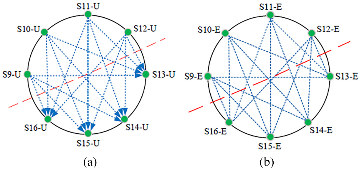
Illustration of the working mode for UEC sensors of the lower layer: (a) ultrasonic part and (b) electrical part.

As shown in Figure 5, the UEC sensors of the lower layer were divided into two groups and labeled as S9–S12 and S13–S16, respectively, where S denotes the UEC sensor, and U and E denote the ultrasonic part and electrical part, respectively. The connecting lines between the U or E parts of different UEC sensors indicate that the two sensors constitute a pair of working sensors, and the arrows for the ultrasonic parts show the propagation direction of the ultrasonic wave. The working mode is explained as below by taking S9 as an example. (1) The electrode of the first UEC sensor on the lower layer is marked as S9-E. The impedance spectra of each electrode pair (i.e. S9-E/S13-E, S9-E/S14-E, S9-E/S15-E, and S9-E/S16-E) are measured in the frequency range of 1 Hz to 20 MHz. (2) The ultrasonic part labeled as S9-U is then stimulated, and S13-U, S14-U, S15-U, and S16-U receive the ultrasonic wave successively for three times.

Experiment and data processing

Experimental materials and procedure

The methane gas with the purity of 99.99% and NaCl solution with the concentration of 3.5% (weight) were used to synthesize the methane hydrate. The unconsolidated sediment was simulated with natural sea sand with the particle size of 0.18–0.25 mm. The porosity was determined at the initial conditions of the experiment. Each run of the experiment was divided into two processes, that is, the synthesis process and decomposition process of methane hydrate. The procedure of each run of the experiment is stated as below:

1. The sea sand was washed and dried before mixing with the NaCl solution. Part of the NaCl solution was used to wet the sand first, and then the wetted sand was filled into the sample vessel layer by layer and compacted with a rubber rod. The sample vessel was closed with the top cover, and all valves on the pipelines connected to the vessel were switched off. A vacuum pump was then connected to the pipeline on the top cover and run for about 1 h to exhaust the air trapped in the vessel. Then, the remained NaCl solution was inhaled into the sand pack through a pipeline on the bottom cover. Finally, the sand pack was saturated with NaCl solution.

2. The piston (shown in Figure 3) was loaded into the sample vessel after detaching the top cover, and the lower end surface of the piston was flattened against the upper surface of the sand pack. A gap formed between the piston and top cover of the vessel, where water was injected to generate a hydraulic pressure with a pump. The hydraulic pressure applied to the sand pack acts as an axial pressure to simulate the overburden pressure in the field. The porosity of the sand pack decreases with the application of the axial pressure; thus, the sand pack became over saturated with the NaCl solution. The excess solution was then drained out through the pipeline on the bottom cover. Then the sand pack recovered into the state of brine saturation. The real porosity of the sand pack was obtained according to the net quantity of the solution inhaled into it.

3. The gas storage tank was connected to the sample vessel first, but the valve between the gas storage tank and sample vessel was closed at the initial stage. The methane gas stored in the high-pressure (around 15 MPa) gas bottle was injected into the gas storage tank slowly until the pressure reached a medium pressure (e.g. 2 MPa). Then the opening of the valve between the gas storage tank and sample vessel was increased gradually to ensure that the gas was injected into the sand pack slowly. After a pressure equilibrium among the high-pressure gas bottle, gas storage tank, and sample vessel was achieved, the outlet pressure of the high-pressure gas bottle was elevated slowly to allow more gas injected into the sand pack and increase the pore fluid pressure. A high pore fluid pressure (e.g. 7 MPa) was required to synthesize the methane hydrate. Then the gas source connection was cut off by closing the valve between the high-pressure gas bottle and gas storage tank.

4. The sample vessel and gas storage tank were placed into a low/constant temperature air bath. A period of time (e.g. 24 h) was necessary to ensure that the methane gas was fully dissolved into the NaCl solution and meanwhile to examine the gas tightness of the gas storage tank and sample vessel. Then a low temperature (e.g. 0.5°C) required to synthesize the hydrate was set to the air bath. The cooling mode of the air bath was triggered and then the Measurement & Control software started to operate. The synthesis process of methane hydrate was initiated. The hydrate synthesis process lasted for several days (e.g. 5 days), and then was terminated by stopping the cooling mode of the air bath. Finally, the decomposition process of methane hydrate started under the condition of room temperature.

Data processing

The raw experimental data (e.g. voltages) were saved during the synthesis and decomposition processes of methane hydrate in the sand pack. Meanwhile, several parameters such as hydrate saturation, speed of the ultrasonic wave, and impedance were calculated. Then typical acoustic and electrical models were adopted to analyze the experimental data.

The hydrate saturation in the sample vessel was calculated based on the gas consumption principle (equation (1)). The consumption of the methane gas was determined through the measured pore pressure and temperature in the sample vessel

$$S_{\mathrm{H}}=\frac{(\frac{P_1{V}_1}{Z_1{T}_1}-\frac{P_2{V}_2}{Z_2{T}_2})M_{\mathrm{H}}}{R_{\mathrm{g}}{\rho }_{\mathrm{H}}{V}_{\mathrm{P}}}\times 100\mathrm{\%}$$

(1)

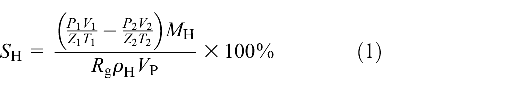
where S_H is the hydrate saturation, %; P, V, and T are the pressure (Pa), volume (m³), and temperature (K) of methane gas, respectively (the subscripts 1 and 2 represent a state without any hydrate and a certain state in the hydrate synthesis process, respectively); M_H and ρ_H are the molar mass and density of methane hydrate (0.122 kg/mol and 910 kg/m³, respectively); V_P is the total pore volume of sand pack, m³; Z is the gas compression factor; and R_g is the ideal gas constant, that is, 8.314 J/(mol·K).

The speed of the ultrasonic wave (sound velocity) was obtained by analyzing the received ultrasound signals. The ultrasound signals were filtered based on the principle of wavelet-transform modulus maxima. ¹⁶ This denoising method has characteristics of strong stability and low noise dependence; thus, it is quite suitable for filtering signals with sudden changes such as the ultrasound signals. Haar wavelet was selected as the wavelet base function based on a comparison with other function series of DB-N, Sym-N, and Coif-N. An accurate identification of the arrival time of ultrasonic wave is the key to calculate the sound velocity. As there is a sudden change showing the location of the arrival time in the received ultrasound signal, signal-processing methods for detecting the singularity of signals can be used to identify the sudden change of the signal amplitude efficiently. The wavelet-transform modulus maxima method with Haar wavelet as the base function was implemented to the ultrasound signals.

The electrical impedance between each pair of electrodes of the UEC sensors can be calculated by manipulating the two sampled voltage signals based on the principle of automatic balanced bridge method. The impedance modulus can be obtained by computing the ratio of the maximums of the two sinusoidal voltage waveforms (equation (2)) and the impedance phase angle is the phase difference of the two waveforms (equation (3))

$$\left|Z\right|=\frac{\left|V_1\right|}{\left|V_2\right|}{R}_3$$

(2)

$${\phi }_{\mathrm{Z}}={\phi }_{\mathrm{V}1}-{\phi }_{\mathrm{V}2}$$

(3)

where |Z| is the impedance modulus, Ω; $\left|V_1\right|$ and $\left|V_2\right|$ are the amplitudes of the two sinusoidal voltage waveforms ( $V_1$ and $V_2$ ), respectively, V; R₃ is the resistance to adjust the measurement range of impedance, Ω; ${\phi }_{\mathrm{Z}}$ , ${\phi }_{\mathrm{V}1}$ , and ${\phi }_{\mathrm{V}2}$ are the phase angles of the electrical impedance, the fundamental components of $V_1$ and $V_2$ , rad.

Results and analysis

Analysis with sound velocity models

The variations of the sound velocity of sediment measured by different pairs of UEC sensors and the hydrate saturation with time are shown in Figure 6. The discrepancies among the measured velocities by different pairs of sensors reveal the non-uniform distribution of gas hydrate in the sediment. The average of the initial sound velocity in the lower layer is around 1600 m/s. Generally, the sound velocity increases with an increasing hydrate saturation and the relationship exhibits nonlinear characteristics. There is a sharp rise at the early stage of the hydrate synthesis process. When the hydrate saturation increases to around 1%, the average sound velocity rises from 1600 to 1921 m/s dramatically. Subsequently, with a further growth of gas hydrate, the increase rate of sound velocity becomes lower. The hydrate saturation reaches around 34.5% when the hydrate synthesis process is terminated. The average sound velocity arrives at 2311 m/s, that is, an increase of about 711 m/s compared with that of the initial state without any hydrate in the sediment.

Figure 6.

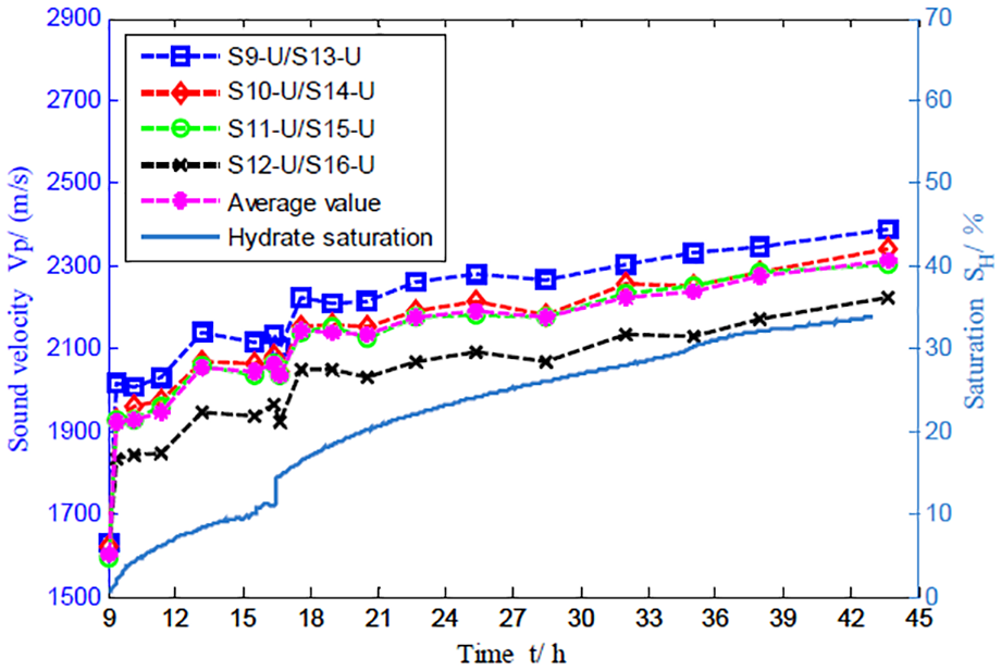
Time traces of the sound velocity and hydrate saturation in the hydrate synthesis process.

The relationship presented by the experimental data was consistent with the previous findings,^17–19 which can be explained by examining the microscopic occurrence mode.^20–22 At the early stage of the hydrate synthesis process, the hydrate cements the sand grain contacts, which increases the contact area between sand grains and enhances the elastic modulus, leading to a sharp increase of sound velocity of the sediment. With the increase of the hydrate saturation, the gas hydrate starts to form in the pore fluid and exhibits a dominant suspension mode that a majority of gas hydrate suspends in the fluid rather than contacting the sand grains directly. Consequently, the contribution of gas hydrate formation to the increase of the elastic modulus is weakened, resulting in a lower increase rate of the sound velocity with hydrate saturation.

The commonly used acoustic models for sound velocity include the time-average equation, ²³ Wood’s equation, ²⁴ and weighted equation. ²⁵ The weighted equation is derived by combining the time-average equation and Wood’s equation. The sound velocity calculated with the three classical models and measured values are shown in Figure 7.

Figure 7.

Comparison of the sound velocity measurements with calculations by typical models.

The time-average equation for the hydrate-bearing sediment is expressed in equation (4). The propagation time in the sediment is taken as the weighted sum of those in the constituents, that is, fluid, hydrate, and matrix

$$\frac{1}{V_{\mathrm{P}}}=\frac{\phi (1-S_{\mathrm{H}})}{V_{\mathrm{W}}}+\frac{\phi S_{\mathrm{H}}}{V_{\mathrm{H}}}+\frac{1-\phi }{V_{\mathrm{M}}}$$

(4)

where V_p is the sound velocity of hydrate-bearing sediment, m/s; φ is the porosity of the sediment; S_H is the hydrate saturation, %; and V_W, V_H, and V_M are the sound velocities of the pore water, hydrate, and sediment matrix, respectively, m/s.

Wood’s equation for the hydrate-bearing sediment is defined in equation (5). The bulk density of the sediment can be calculated through a weighted average of the constituent components, as shown in equation (6)

$$\frac{1}{\rho {V_{\mathrm{P}}}^2}=\frac{\phi (1-S_{\mathrm{H}})}{{\rho }_{\mathrm{W}}{V_{\mathrm{W}}}^2}+\frac{\phi S_{\mathrm{H}}}{{\rho }_{\mathrm{H}}{V_{\mathrm{H}}}^2}+\frac{1-\phi }{{\rho }_{\mathrm{M}}{V_{\mathrm{M}}}^2}$$

(5)

$$\rho =(1-\phi ){\rho }_{\mathrm{M}}+(1-S_{\mathrm{H}})\phi {\rho }_{\mathrm{W}}+S_{\mathrm{H}}\phi {\rho }_{\mathrm{H}}$$

(6)

where ρ, ρ_W, ρ_H, and ρ_M are the densities of the sediment, pore water, hydrate, and sediment matrix, respectively, kg/m³.

The weighted equation is the weighted average of equations (4) and (5), which can be written as equation (7). A weighting factor W and an exponential constant N simulating the rate of lithification related with the hydrate saturation are utilized to provide flexibility in real applications

$$\frac{1}{V_{\mathrm{P}}}=\frac{W\phi {(1-S_{\mathrm{H}})}^N}{V_{\mathrm{P}1}}+\frac{1-W\phi {(1-S_{\mathrm{H}})}^N}{V_{\mathrm{P}2}}$$

(7)

where V_p is the sound velocity of sediment, m/s; V_P1 is the sound velocity calculated with Wood’s equation, m/s; and V_P2 is the velocity calculated with the time-average equation, m/s.

It can be observed in Figure 7 that the time-average equation and Wood’s equation overestimate and underestimate the sound velocity, respectively, and the measured velocity can be fitted well by the weighted equation. The time-average equation is more applicable to conditions that the hydrate cements the grain contacts. The estimated sound velocity of the matrix with the porosity of zero is usually higher than the reality. The time-average equation with velocities of 4370 m/s, 3650 m/s and 1500 m/s for the matrix, hydrate and water respectively presents an upper limit of the calculated sound velocities of hydrate-bearing sediment. Wood’s equation is more applicable to the case with particles in a suspension mode, and thus may be more accurate if the hydrate suspends in the pore fluid. Consequently, with the same estimated matrix velocity as the input, Wood’s equation gives a lower limit of the calculated sound velocities of hydrate-bearing sediment. In reality, both the cementation and suspension modes exist in the synthesis process of gas hydrate. Thus, it is difficult for each of the time-average equation and Wood’s equation to give an accurate calculation of the sound velocity of hydrate-bearing sediment. Alternatively, the weighted equation performs the best because both modes have been taken into account and parameters such as W and N can be flexibly adjusted for a necessary optimization (W = 1.4 and N = 0.5 in this work).

Analysis with Archie’s model

The variations of the impedance modulus and the hydrate saturation with time are shown in Figure 8. Similar to the case of the sound velocity measurements in the “Analysis with sound velocity models” section, the discrepancies among the measured impedance by different pairs of sensors indicate the non-uniform distribution of gas hydrate in the sediment. Generally, the impedance modulus presents a non-monotonic behavior with the increase of hydrate saturation. Three stages can be identified based on the variation characteristics of the impedance modulus. In the first stage, that is, 9–17 h, there is a decrease in the impedance modulus as the hydrate saturation increases from 0% to 10%. The impedance modulus increases sharply with an increase of the hydrate saturation from 10% to 15% in the second stage, that is, 17–18 h, where a rapid growth rate of hydrate emerges. Then a moderate growth of the impedance modulus with the hydrate saturation (higher than 15%) can be seen in the third stage, that is, 18 h afterward.

Figure 8.

Time traces of the impedance modulus (50 kHz) and hydrate saturation in the hydrate synthesis process.

The variation characteristics of the impedance modulus are affected by several factors such as the hydrate saturation, salt-exclusion effect, and temperature. In the first stage, a small amount of hydrate cements the sand grain contacts first, and then grows in the pore space with reference to the analysis of the sound velocity in the “Analysis with sound velocity models” section. The small amount of hydrate is not able to block the connections between pores; thus, the influence on the impedance modulus by the accumulation of hydrate is not as significant as that by the salt-exclusion effect. As a result, an observable drop of the impedance modulus is induced by the joint effect of hydrate-accumulation and salt-exclusion. In the second stage, a significant portion of the pore connections is blocked due to a rapid and continuous growth of gas hydrate. The sharp increase of the impedance modulus is attributed to at least two mechanisms. The dominant mechanism is that the high-resistivity hydrate blocks the migration path of ions in the conductive pore fluid; thus, the electrical resistance rises significantly. The secondary mechanism is that the hydrate suspending in the pore fluid increases the contact area between solid particles (including both sand and hydrate particles) and solution, by which a stronger interfacial polarization effect is induced leading to an increase in the capacitance. In the third stage, with a continuous growth of gas hydrate, the blocking effect decays leading to a moderate growth of the impedance modulus because only a minor portion of pore connections left open after the second stage.

Archie’s formula is a model that relates the porosity, water saturation, and resistivity of sandstone.^26–28 The resistivity in the original formula is replaced by the impedance modulus in this study. The impedance describes both the capacitance and resistance characteristics of the sediment under test. According to the original Archie’s formula, the proportional coefficient between the impedance of the water-saturated sandstone and that of the pore water is defined to be formation factor, as expressed in equation (8)

$$F=\frac{Z_{\mathrm{O}}}{Z_{\mathrm{W}}}=\frac{a}{{\phi }^m}$$

(8)

where F is the formation factor; Z_O is the impedance modulus of sediment saturated with water completely, Ω; Z_W is the impedance modulus of the pore water, Ω; m is the cementation index (m = 1.15 in this work); and a is a coefficient related to lithological properties (a = 1 in this work). The impedance index analogue to the resistivity index in the original Archie’s formula is expressed in equation (9)

$$I=\frac{Z_{\mathrm{t}}}{Z_{\mathrm{O}}}=\frac{b}{{S_{\mathrm{W}}}^n}$$

(9)

where I is the impedance index; Z_t is the impedance modulus of hydrate-bearing sediment (partially saturated with water), Ω; b is a coefficient related to lithological properties; n is the saturation index; and S_W is the water saturation (S_W = 1 – S_H), %. By multiplying F and I, an expression for calculating the hydrate saturation can be obtained, as shown in equation (10)

$$S_{\mathrm{H}}=1-{\left(\frac{b{Z}_{\mathrm{W}}}{Z_{\mathrm{t}}{\phi }^m}\right)}^{\frac{1}{n}}$$

(10)

It needs to be stressed that the electrical impedance is affected by the salt-exclusion effect significantly. As a result, the relation between the impedance modulus and hydrate saturation is not monotonous. Therefore, in this work, a segmented regression method based on the experimental data is adopted to obtain the values of the parameters of Archie’s model, that is, b and n in equation (10). Figure 9 compares the measured impedance and model calculated values at different hydrate saturations. The relationship between the impedance modulus and hydrate saturation can be divided into two segments with S_H = 15% as the demarcation point. The model parameters b and n are 1.2516 and −0.5984 for S_H < 15%, and 1.3232 and 1.6834 for S_H > 15%, respectively.

Figure 9.

Comparison of the impedance measurements with calculations by Archie’s model.

Conclusion

An experimental system called UCEI was developed for jointly testing the ultrasonic wave parameters and electrical impedance of hydrate-bearing porous media during the course of hydrate formation and decomposition. Experiment was carried out with methane gas as the hydrate former, and the acoustic and electrical parameters of hydrate-bearing porous medium were derived by processing the experimental data. The acoustic and electrical properties were analyzed with typical acoustic models (the time-average equation, Wood’s equation, and weighted equation) and Archie’s formula.

1. The UCEI system features its novel UEC sensors and sensor array, fully controllable instruments, variety of sampled data, and flexible working modes. Key parameters such as the sound velocity and electrical impedance can be obtained jointly from the identical measured object, without any intrusion/disturbance to the object, at different orientations in space. The parameters can be used to characterize the acoustic and electrical properties of hydrate-bearing sediments conjointly.

2. An appropriate denoising method is required to preprocess the sampled data especially in the case of sound velocity calculation from the ultrasound waveforms. The wavelet-analysis based denoising approach and singularity detection method with Haar wavelet as the base function for both are effective means to filter the ultrasound signals and identify the arriving time of the ultrasonic wave.

3. The measured sound velocity and electrical impedance can quantitatively characterize the hydrate-bearing sediment correctly, which demonstrates the applicability of the developed UCEI system. The weighted equation is recommended for modeling the sound velocity because both cementation and suspension modes are taken into account, and the adjustable model parameters add more flexibility for data fitting. Archie’s formula can be used to model the modulus of electrical impedance; however, a segmented regression method should be utilized because there is a non-monotonic relationship between the impedance modulus and hydrate saturation induced by the salt-exclusion effect in the hydrate synthesis process.