
Abstract
Resilience provides a new approach that system administrators can use in the design and analysis of engineering systems to enhance the ability of such systems to withstand uncertain threats. In this article, an improved integrated metric is proposed for the quantitative assessment of resilience. The proposed metric is constructed in the form of a summation of two capacities: absorptive and restorative capacities. A weight coefficient is assigned to each capacity to enhance the flexibility according to various system requirements of stakeholders. In addition, based on the absolute time scale, a new time factor is proposed and incorporated into the resilience metric to quantify the effect of time on system performance. To test the performance of the proposed metric, three experimental studies are conducted wherein the proposed metric is compared with two other metrics reported in the literature. The results indicate that the proposed metric extends the flexibility of the previous metrics to systems where the time scale is addressed, and that the numerical values of resilience lie in a proper range and can be compared conveniently across different engineering systems. Furthermore, an example of an information exchange network is adopted to demonstrate the applicability of the proposed metric.
Keywords
Introduction
The term ‘resilience’ was first proposed by Holling 1 in the study of ecological systems. Since then, the concept of resilience and its evaluation methods have been developed and applied to many real-world complex systems such as national infrastructure facilities,2–4 ecological systems5,6 and economic systems.7,8 In addition, resilience has expanded the library of system attributes such as reliability, robustness, safety and risk. Resilience is commonly studied to assess and improve the capability of a system to bounce back from disruptive events to its normal condition.9,10 Currently, the development of resilience in complex engineering systems is still in its early stage. Several reported works have made some progress in defining and evaluating resilience for complex engineering systems.
The definitions of resilience reported so far can be classified into two types. One type approaches resilience from a specific disciplinary perspective. 7 This type of definitions may address various aspects of system resilience due to changes in specific systems, which is appropriate for particular domains but may not be suitable for other applications. The other type approaches resilience from a more general perspective.11–14 This type of definitions can be applied to various engineering systems. For instance, Vugrin et al. 11 defined resilience as a function of the absorptive, adaptive and restorative capacities. The absorptive capacity is the degree to which a system is able to absorb shocks caused by external disruption. The adaptive capacity is the degree to which a system is able to adapt itself temporarily to new disrupted conditions. The restorative capacity is the degree to which a system is able to restore itself if the adaptive capacity is not effective. This definition addresses the abilities of the system to resist disruptive events and ensure timely restoration.12,14 Note that the adaptive and restorative capacities refer to recovery activities and that the effects of these capacities overlap in the recovery phase. Hence, in this study, the adaptive capacity is merged with the restorative capacity to describe the dynamic behaviour of system performance in the system recovery phase.
Compared to the definitions of resilience, the assessment methods for resilience seem to have attracted more attention from engineers and practitioners. In general, resilience assessment methods can be separated into two major categories: qualitative and quantitative methods. 15 The qualitative category includes methods that tend to assess the system resilience without numerical descriptors. For more information on qualitative resilience assessment methods, readers can refer to previous literature.16–20
The first general quantitative assessment method was proposed by Bruneau et al., 21 who aimed to measure the seismic resilience of a community to an earthquake by estimating the expected degradation in the quality of community infrastructure. They proposed a deterministic static metric for measuring the resilience loss of a community to an earthquake. In this pioneering research work, the concept of resilience loss, also known as a ‘resilience triangle’, was proposed, and has been widely utilized as a fundamental guide for quantitative resilience assessment methods.22–25 Although this approach is utilized for the context of an earthquake, it has the advantage of general applicability and can be extended to many systems.
However, these resilience triangle paradigms are relatively simple and may not be able to represent the dynamic behaviours of various systems. For example, the resilience metric in Bruneau et al.’s study assumes that the normal quality of community infrastructure is at 100%. This assumption is unrealistic because the reference standard is difficult to quantify for practical systems.
Henry and Ramirez-Marquez 26 use three system states – stable original state, disrupted state and stable recovered state – to quantifying system resilience. The advantage of this metric is that both the disruption and recovery phases are considered. Similar time-dependent metrics have been adopted in other studies.27–29 However, these time-dependent metrics perform poorly in representing the global level of system resilience intuitionally in comparison to metrics presented as a single numerical value.
Practically, a general resilience metric should satisfy the requirements of both comprehensiveness and universality. Comprehensiveness refers to the ability to capture the essence of system resilience and ensure that the quantification of resilience is consistent with its associated concepts. For instance, a general metric should be able to identify the variations in system performance precisely via its calculated results. Universality refers to the proper form of a resilience metric. For instance, a metric presented as a calculated value is better than a metric presented as a function of time. In addition, a metric value with a finite close domain such as [0, 1] is preferred to a metric with an infinite domain such as [0,
Recently, several studies have investigated the comprehensiveness and universality of resilience metrics. Nan and Sansavini 13 proposed an integrated metric for assessing the resilience of interdependent infrastructures. Their proposed metric consists of several factors, which are measured from the aspects of the time scale and performance level. Each factor is consistent with the concept of the defined resilience capacities, and the resilience metric has a range of [0,). Tran et al.30,31 proposed a novel resilience metric in which each factor is compatibly constructed. An improvement of Tran et al.’s metric over Nan and Sansavini’s is that it has a reference value of 2 when no disruptive event occurs.
However, the resilience metrics proposed by Nan and Sansavini 13 and Tran et al.30,31 have two shortcomings. First, their metrics use a relative time scale to model the time factor. This may cause problems because many realistic systems, such as infrastructure systems affected by an earthquake, concern only the absolute time scale. Second, the quantification of the absorptive capacity and that of the restorative capacity overlap each other, which leads to poor performance in scenarios that address the difference between these two capacities. For instance, the absorptive capacity is often emphasized more in an ecological system because the recovery of ecological losses involves huge economic costs and requires a long time, whereas the restorative capacity is more emphasized in a military C2 network because timeliness is essential in the military. Note that these problems also exist in previous resilience metrics.32–35
Thus, in this study, we aim to develop an improved integrated metric that overcomes the disadvantages existing in previous metrics.32–35 The major contributions of this article are summarized as follows:
Based on the absolute time scale, a new time factor is proposed and incorporated into the resilience metric to quantify the effect of time on system performance.
The absorptive and restorative capacities are used to quantify the proposed resilience metric in the form of a summation. Two weight coefficients are assigned to the two capacities to enhance the flexibility of the proposed metric according to various system requirements of stakeholders.
Each capacity is quantified from the perspective of state transition because of the dynamic behaviour during the disruption and recovery phases. Three dimensions – transition process, transition time and transition consequence – are used to describe the resilience capacities.
The proposed metric is compared and discussed using experimental scenarios.
A case study on information exchange in a networked engineering system is conducted to validate the proposed metric.
The rest of this article is organized as follows. Section ‘Development of improved integrated metric’ describes the development of the proposed integrated resilience metric. Section ‘Experimental comparison’ presents the comparison of the proposed metric with previously reported ones using three scenarios. Section ‘Case study on information exchange in networked system’ presents a case study on information exchange in a networked system to demonstrate the application of the proposed metric. Section ‘Conclusion’ concludes this article.
Development of improved integrated metric
In this section, we present the development of an improved integrated metric for resilience based on system performance. First, we describe the system performance measure. Second, we present the improved resilience metric.
System performance measure
In this study, an example involving notional system performance data is used to illustrate the construction of the resilience metric, as shown in Figure 1. Because the performance data are notional and can be replaced by real performance data from practical engineering systems, the resilience metric constructed on the basis of such performance data can also be adapted to various systems. The abscissa represents the time t, and the ordinate represents the performance data
td = time when the disruption event starts;
tr = time when the recovery action starts;
ts = time when the recovery performance reaches a steady state;
yo = normal operating performance level;
ymin = minimum performance level;
ys = recovered performance level.
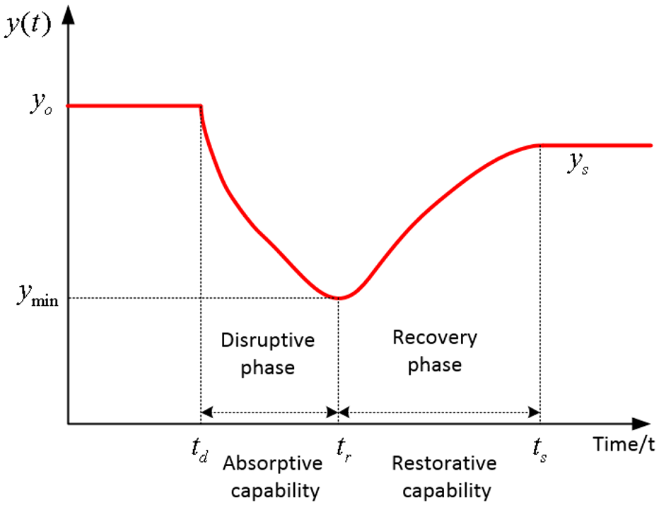
Notional plot of system performance data over time during disruption and recovery phases.
The system performance is assumed to be at a normal operating level before a disruption event occurs. When the disruption event occurs at time
Improved metric
When a disruption event or recovery action is applied to a resilient system, the system will transition from one stable state to another stable one. Normally, three important aspects are considered during the transition period. The first aspect is the manner in which the transition is carried out, which describes the transition process of the system performance. The second aspect is the level to which the system state reaches compared to the initial level. The last aspect is the time taken to finish the transition process. Once these three aspects of the transition period are determined, the absorptive and restorative capacities of the system can be quantified.
By considering these three aspects, both the absorptive and restorative capacities of the system resilience are measured by the process, time and consequence factors. The disruption process factor
After all the factors are determined, an integrated resilience metric is developed to quantify the system resilience as follows

where
Disruption process factor
The disruption process factor

As can be seen, it is measured precisely using the performance data during the disruption phase. Hence, the dynamic behaviour of the system performance during the disruption process can be captured. For instance, consider the three cases shown in Figure 2; when these three cases differ only in the dynamic performance behaviour during the disruption phase, the resilience of the three cases follows the order case 1 > case 2 > case 3, which can be reflected using equation (2).
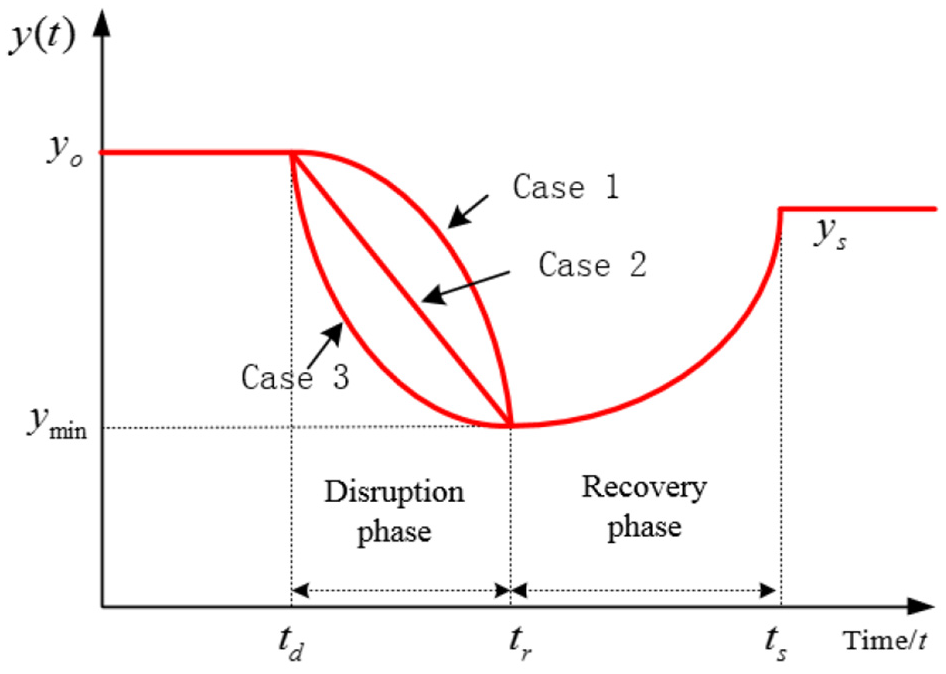
Illustration of systems having different performance behaviours during disruption phase.
Disruption consequence factor
The disruption consequence factor

The minimum performance
Disruption time factor
The disruption process factor and disruption consequence factor can capture the absorptive capacity of system resilience effectively from the perspective of system performance. However, a measure from the perspective of time has not been considered, although it is another necessarily significant aspect for assessing system resilience. Various measures have been introduced to quantify the time effect on system resilience. For instance, a time factor has been represented by a function of time30,34 or incorporated into a function of both time and performance. 13 Previous studies used the relative time scale to quantify the time factor. The advantage is that the time factor becomes dimensionless. Thus, the factors derived from both the time and performance dimensions can be integrated into an integrated metric, in which the performance factor is also dimensionless.
However, the quantification of the time factor in a relative scale may incur problems because many realistic systems are only concerned with the absolute time scale. Figure 3 illustrates the system performance in two cases with different time periods. In case 1, the dynamic performance is carried out in the same manner as that in case 2; however, the time taken in case 1 is only half of that taken in case 2. By fixing the other conditions for both cases, it is natural to conclude that the system performs better in case 1 in terms of system resilience because the resilience is rewarded when the period is shorter in the transition process. However, for metrics using the relative time scale, a conclusion that the two cases have the same resilience would be obtained because the time difference between the cases cannot be reflected. Consequently, metrics that adopt relative time scale factors are not appropriate in such a scenario.

Illustration of system performance in two cases with different periods.
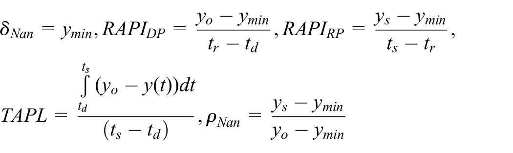
In response to the above discussion, a novel time factor that is calculated using the absolute time scale is proposed as follows

where
Recovery process, consequence and time factors
The three aspects of the recovery capacity, that is, the recovery process factor, recovery consequence factor and recovery time factor, are defined in a manner similar to those of the absorptive capacity. The recovery process factor accounts for the total performance maintained by a system through the recovery phase and is given by equation (5). As shown in equation (6), the recovery consequence factor is defined as the ratio of the recovered performance level to the desired performance level. The recovery time factor is defined in a similar manner to the disruption time factor, except that the recovered time


Noticeably, the measure of the restorative and absorptive capacities are almost symmetric. Each capacity is measured in both the time and performance dimensions using three quantified factors. The three quantified factors are all normalized and dimensionless and have the same reference value of one during normal operation. Hence, it is easy to integrate the three factors to quantify the restorative and absorptive capacities. Furthermore, no overlap occurs among the three factors.
Experimental comparison
Three experimental studies are conducted by comparing the proposed metric with two reported resilience metrics by Tran et al. 30 and Nan and Sansavini. 13 They share the following common characteristics:
All the three metrics are derived from the same notional performance data shown in Figure 1.
The absorptive and restorative capacities are considered as measures of system resilience and are quantified using performance data.
All the factors are integrated into a single metric.
Preliminary details of two reported metrics
The two reported metrics are introduced briefly here. Readers can refer to previous literature13,30 for more details. The resilience metric proposed by Tran et al. 30 is given as follows
where
The total performance factor
The resilience metric proposed by Nan and Sansavini 13 is given as follows

where
As can be seen, the robustness factor
In general, the comparisons of the three resilience metrics in terms of the time, process and consequence factors are summarized in Table 1. Our proposed metric mainly differs in the time and process factors. Instead of the relative time scale, the absolute time scale is adopted for the time factor in this study. The process factor of Tran et al. 30 and Nan and Sansavini 13 is measured using the entire performance data for both the phases. In contrast, two process factors are proposed in this study to measure the dynamic behaviour of system performance separately for the disruption and recovery phases.
Comparison of the three resilience metrics.

Comparison of metrics in three experimental scenarios
Scenario 1
Scenario 1 considers the two cases described in section ‘Disruption time factor’ (Figure 3). In case 1, the dynamic performance is carried out in the same manner as that in case 2; however, the time taken in case 1 is only half of that taken in case 2. The performance data for cases 1 and 2 are created using the same logistic function used by Tran et al. 30 A disruption with no recovery action for the system is represented using notional performance data generated by the following equation

where

where a negative sign is added in front of
Logistic function parameters are used to change the shape of the performance data. Considering that the disruption and recovery actions are the same in this scenario, only the parameter of the recovered level

Notional performance data generated by equations (10) and (11) for different recovered levels
The performance data of the six scenarios during the disruption phase (0–50 time steps) in case 1 are generated with the same equation (10). As a result, the performance lines with various markers are plotted coincidently, which resulted in such ‘hexagon star’ presentation. This phenomenon also occurs in case 2 during the disruption phase (0–70 time steps).
Figure 5 shows the calculated results of the three metrics for cases 1 and 2 with different recovered performance level

Resilience results for cases 1 and 2 obtained using the three resilience metrics.
As previously mentioned, resilience is rewarded when the time period is shorter in the transition process. When the other conditions are kept constant for both the cases, the system performs better in case 1 in terms of the system resilience. Thus, the relative time scale factor in
Scenario 2
Scenario 2 considers three cases for the performance data, as illustrated in Figure 6. The desired performance level

Performance data for three cases where parameters
Table 2 lists the resilience results calculated by the three metrics. The results of
Resilience calculation for scenario 2 using the three metrics.
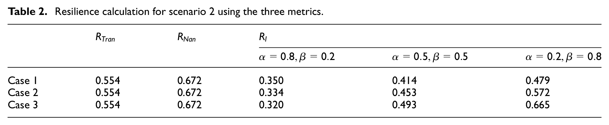
For the metric
For the metric
Note that when
Scenario 3
Scenario 3 considers the performance data for four cases, as illustrated in Figure 7. For cases 1–3, all factors except the initial moment of recovery time are the same. Case 4 undergoes the same disruption phase as case 2 and the same recovery phase as case 1. The disruption time for cases 1–3 follows the order case 1 < case 2 < case 3, indicating that the absorptive capacity for case 3 is the highest. Similarly, case 3 has the highest restorative capacity among cases 1–3 because it takes the least time.

Performance data for four cases where parameters
Table 3 lists the resilience results calculated by the three metrics. The resilience values obtained by the metric
Resilience calculation for four cases using three metrics.

For the metric
Case study on information exchange in networked system
The application of the proposed resilience metric is demonstrated using a model of information exchange in a networked system. Many networked systems such as the Internet, World Wide Web, organizational networks and social networks rely on information exchange to facilitate the overall performance of the system. However, the connectivity can be vulnerable to disruptions, leading to node and/or link failures as well as degradation in system performance. In this study, a model proposed by Dodds et al. 36 to study organizational networks is used to simulate information exchange in a network. The information exchange has also been adopted by Tran et al., 30 who define network disruptions as node removal events and recovery strategies as link rewiring. The proposed resilience metric, as applied to this problem of information exchange in networked systems, includes the system description, analysis of potential disruptions and recovery action and system performance measurement.
System description of information exchange in networks of interest
The system of interest can be represented as a network, which consists of nodes and links. Nodes are individual members within a system, and links are potential paths of information flow. A model based on the one adopted in previous studies30,36 is used to simulate information exchange in a network. The goal of the networked system is to successfully enable information sharing between nodes during the operation period.
Scale-free network is adopted for network topology initialization because of its existence in many real-world complex systems.37,38 The scale-free topology is created using the Barabási–Albert (BA) preferential attachment model.
39
The BA model begins with a small number of initially connected nodes (
Information exchange is realized by passing messages from the source node to the sink node. Each node in the network creates a new message with probability
Analysis of disruption and recovery action in networks of interest
Node removals are considered as disruption events. Nodes can be removed uniformly at random, that is, random node failures, or in a targeted manner, that is, intentional network attacks. Targeted node removal is based on the node degree; nodes with the highest node degrees are removed each time. Node degrees are recalculated following any changes to the network topology.
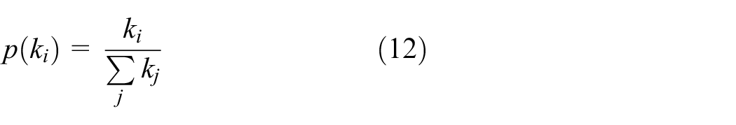
The recovery actions considered in this study focus on link rewiring, wherein nodes affected by a disruption rewire any links disconnected by the disruption. Two recovery strategies are considered: random rewiring and preferential attachment. In random rewiring, disconnected nodes randomly decide whom they rewire to. In preferential attachment, disconnected nodes decide whom they rewire based on the probability equation given by equation (12), which gives preference to highly connected nodes.
Node removals and recovery actions are implemented within quantitative time steps. For instance, a disruption event lasting from time
System performance measurement for information exchange networks
The system performance
Six scenarios are considered in this case, as listed in Table 4. The initial network topologies are all scale-free, with networks being subjected to a disruption event during the period of 50–70 time steps. Node removal occurs every five time steps during the disruption phase, with r nodes being removed each time. In scenarios with a recovery action, the recovery phase lasts for 90–110 time steps. Link rewiring occurs every five time steps during the recovery phase, with disconnected links being rewired in an order of time. The rewiring order is such that the links disconnected earliest are linked first. Considering the stochasticity of the simulation, 100 repetitions are run for each scenario. Stochasticity in the simulation is a result of randomness in message generation, the BA algorithm, node removals and link rewiring. Hence, statistical analysis of the output simulation data is carried out to characterize the resulting uncertainty in system performance.
Resilience of information exchange networks under different disruption and recovery strategies.
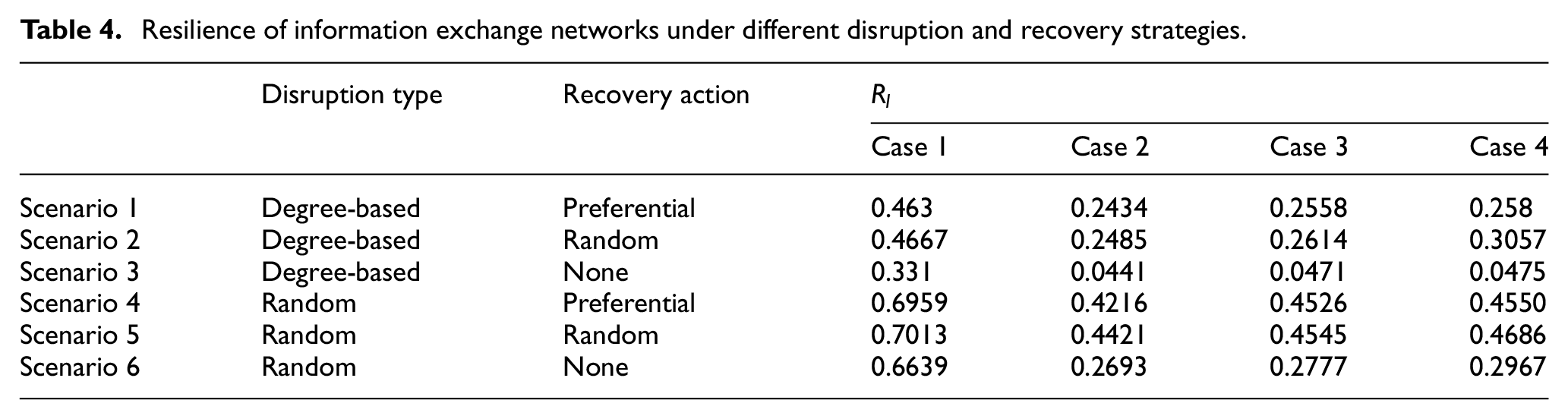
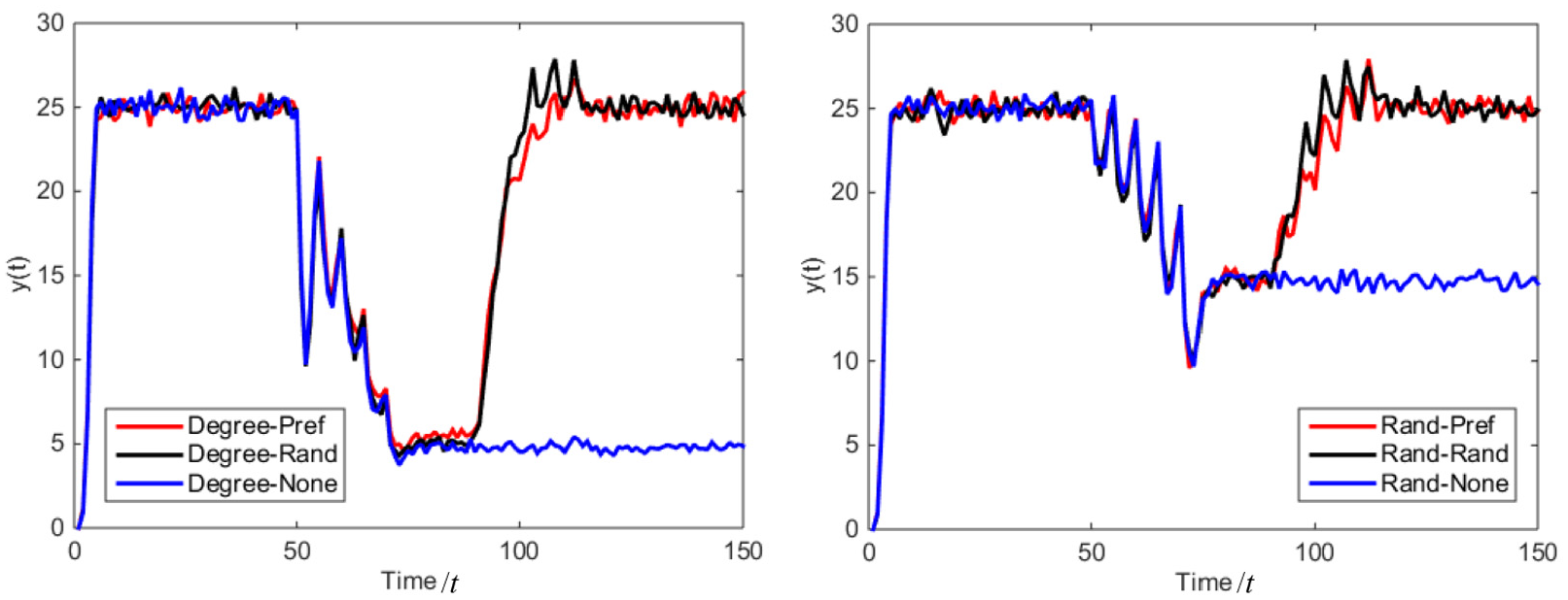
Figure 8 shows the mean performance data for each of the considered scenarios. The initial network topologies are created using the BA model, with

Case 1: Mean performance data for networks subjected to (a) degree-based (Degree) attacks and (b) random attacks. Two adaptation strategies are considered – random (Rand) and preferential attachment (Pref) – in addition to no recovery action (None).
Different values for parameter r are considered to study the effect of removed nodes number on the information exchange network performance. Three other cases of node removal are adopted: (1) r is kept constant at 10 during the removal process; (2) r increases linearly with the occurrence frequency of node removal, with an initial value of
Case 2: Linear increase in number of removed nodes r with occurrence frequency of node removal, with initial value of

Case 3: Constant number of removed nodes (

Case 4: Linear decrease in number of removed nodes
r
with occurrence frequency of node removal, with initial value of
Figures 9–11 show that though the performance data during the disruption period for the three cases are different, it is difficult to determine whose resilience is the highest from the performance plots. Hence, the proposed resilience metric is used for further quantitative analysis. Table 4 lists the resilience values calculated by metric
Conclusion
This article presents an improved metric for the quantitative assessment of system resilience based on the system absorptive capacity and system restorative capacity. Each capacity is evaluated from the perspective of state transition and quantified by the time, process and consequence factors. The proposed metric has three advantages. First, a new time factor is proposed and incorporated into the resilience metric to quantify the effect of time on system performance. Second, system resilience is classified into two capacities based on the classification of the disruption and restoration phases. Two weight coefficients are assigned to the two capacities, which enhance the flexibility of the proposed metric when the stakeholder has different requirements for the absorptive and restorative capacities. Third, the numerical values of resilience under the proposed metric lie in a proper range and can be compared conveniently across different engineering systems. Three scenarios are used to validate the performance of the proposed metric, wherein the metric is compared with two previously reported metrics. In addition, an example of information exchange networks is used to demonstrate the application of the proposed metric.
The proposed resilience metric does not consider the cost benefit analysis and threat probabilities. For example, given knowledge of specific threat likelihoods, a system designer cannot use the assessments produced by our metric to determine whether enhancing the absorptive capacity or the restorative capacity can improve the system resilience in an economic manner. In addition, the proposed metric may cause confusion due to the summing form of two capacities and the imbalance of the two weight coefficients. We plan to improve the proposed metric in our future study. These aspects will be dealt with in future studies by improving the proposed metric.
Footnotes
Handling Editor: James Baldwin
Declaration of conflicting interests
The author(s) declared no potential conflicts of interest with respect to the research, authorship and/or publication of this article.
Funding
The author(s) disclosed receipt of the following financial support for the research, authorship and/or publication of this article: This work was supported by the National Natural Science Foundation of China (grant numbers: 71701207 and 51705526), the National Defence Science and Technology Project Fund of the Central Military Commission (grant number: 3101097) and Science & Technology on Reliability & Environmental Engineering Laboratory.