A method for assessing wheel fatigue reliability considering multiaxial stress state

Abstract

Electric multiple unit is a modern transportation tool with high efficiency and large carrying capacity. Regarding its high speed, reliability requirement of the train is very important. As the main load bearing component of a train, the wheel is subjected to harsh working condition. Rolling contact between wheel and rail leads to wheel fatigue failure so that the fatigue reliability of wheel becomes one of the most attractive fields in electric multiple unit reliability study. This article proposed a fatigue reliability assessment method. It could obtain critical parts’ stress distribution efficiently through the force–stress relationship received by numerical simulation, so that it could assess wheel fatigue reliability under measured force–time spectrum. Also, multiaxial fatigue is considered in the method and the equivalent stress can be obtained by multiaxial model and fatigue experiment. Result of the case study shows that fatigue reliability of China Railway High-speed 5 wheel at 60,000 km mileage is 68%.

Introduction

China Railway High-speed (CRH) is the world largest high-speed railway system. Founded in 2002, China now has the longest operation length of high-speed railway, which is about 20,000 km around the world. ¹ China Railway High-speed 5 (CRH5) electric multiple unit (EMU) is a low-temperature-type train which is used in Northeast China where the lowest temperature is below −40°C. Wheel, as part of train, is more likely to fail compared to other parts of the train due to its harsh working environment. Under heavy-load, high-speed, and low-temperature conditions, if the reliability of the wheel is sufficient to guarantee safety operation is questionable.

Numerous papers dealing with wheel reliability assessment could be found in the literature.^2–5 Besides, Liu et al. ⁶ used multiaxial fatigue analysis combined with Monte Carlo simulation to investigate the reliability of train wheels. Zhao ⁷ evaluated the fatigue reliability of axles of Chinese railway vehicles through stress–strength interference theory. This work was simple to implement, giving the failure probability with a quite acceptable computational time and providing useful information with regard to the quantification of the failure probability of the component. ⁸ While, no matter which method is used, stress and strength distributions of the critical part are indispensable.

Strength distribution could be derived by probabilistic confidence stress life (PCSN) curves if the life distribution was known in advance. PCSN curves are the base of reliability estimation and should be obtained first. To get PCSN curves, experts often used experiments and statistics extrapolation. In other words, they obtained the low- and high-cycle fatigue range curves by experiment then extrapolated the curves to very high cycle fatigue (VHCF) range in consideration of the extraordinarily time-consuming experimental process in VHCF stage. Consequently, the accuracy of extrapolation methods influences the quality of whole PCSN curves directly. There are three main extrapolation methods: American Association of State Highway and Transportation Officials (AASHTO), European Convention for Constructional Steel Work (ECCS), and concurrent probabilistic method (CPM). AASHTO standard was a US national standard which directly applies the S-N curve generated by experiment data in the low and high life range into the super high region. ⁹ ECCS suggested that the exponent m of the S-N curve in the low and high life region should be applied in the form of 2m − 1 in the super high life range, after a fatigue life of 5E6 cycles. ¹⁰ However, these two extrapolation methods are too conservative comparing with CPM method. CPM, proposed by Zhao et al., ¹¹ was used to extrapolate more precise curves and had been successfully used in many researches. Zhao ⁷ obtained strength probability density function (PDF) from PCSN relationships. Subsequently, J Klemenc ¹² called this method as “two-phase procedure” and compared it with “direct procedure”; he found that the former one was more precise than the latter one. Therefore, CPM was used as extrapolation method and the “two-phase procedure” was applied to deduce the strength distribution in this article.

To get a stress distribution, the force history should be obtained in prior. Generally, sensor is placed in the structure to receive force history. Liang ¹³ applied a polynomial to convert the measured wheel force into stress in dangerous point. ND Adasooriya ¹⁴ used rainflow counting to process the measured stress spectrum of railway truss bridge and fit the stress distribution. However, measured load spectrum from a key point on structure is not always applicable. Multibody dynamic (MBD) simulation is another way to get force spectrum and is suitable for most of cases.

Usually, it is time-consuming to receive a stress spectrum from the MBD simulated force spectrum using a finite element analysis because the force is time-varying. Meanwhile, the stress state of wheel under operation is complex, and it is known as the multiaxial stress state. How to describe the stress distribution under multiaxial stress state and time-varying force properly and efficiently is a key factor for reliability assessment. To solve this problem, a method to obtain stress distribution under multiaxial stress state was proposed, and combined with the strength distribution obtained from fatigue test, fatigue reliability of wheel was assessed. In this article, section “Introduction” introduced the different reliability calculation methods; section “Material and methods” described the fatigue reliability assessment method; section “Results and discussion” was a case study of the CRH5 wheel fatigue reliability assessment; and section “Conclusion” drawn conclusions of the article.

Material and methods

Fatigue reliability assessment method

Figure 1 shows the flowchart of the reliability assessment method proposed in this article. The reliability was obtained by interference of the stress distribution with strength distribution of component. According to the picture, stress distribution is obtained by numerical simulation, while strength distribution is based on the fatigue test and numerical extrapolation.

Figure 1.

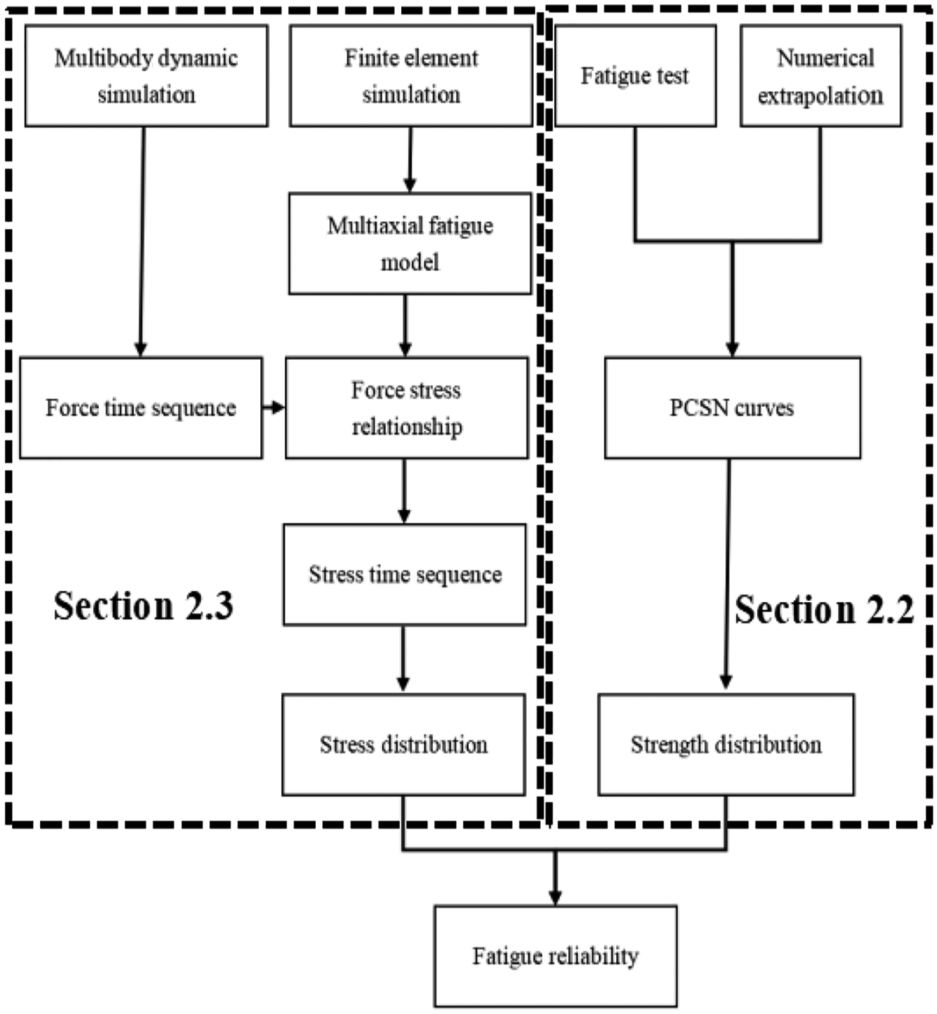
Flowchart of the reliability assessment method.

The method could be divided into two main parts: the sections “Material fatigue tests and strength distribution” and “Multiaxial stress state and stress distribution” would describe the two parts in detail. By introducing the force–stress relationship in this article, the advantage of the proposed method was that it could assess the fatigue reliability of wheel under variable vertical force obtained whether by measurement or simulation.

Material fatigue tests and strength distribution

Tension–compression fatigue test was conducted in this article. Totally 5–7 stress levels were selected with 3–5 specimens each level. Besides, up-and-down test is used to obtain fatigue limit at different load types. The test needs at least seven pairs of specimens, and the run out number of cycle is 5E6 here in the method. After finishing the test, CPM method is used as the numerical extrapolation method to get whole PCSN curves in this article. CPM method uses two parts to describe the whole PCSN curves of materials in log–log coordination. The first part is obtained by fatigue experiments, which represents the low- and high-cycle fatigue range, and the second part is through extrapolation at a translation point N_T which represents the VHCF region.

To obtain the first part of PCSN curves of R8T at −40°C, the test data should be first processed by general maximum likelihood method and the procedures are as follows. From

$$S^{m}N=D$$

(1)

Taking a logarithm to both sides of equation (1)

$$\lg N=\lg D-m\lg S$$

(2)

Set Y = lgN, A = lgD, B = −m, and equation (2) can be written as

$$\{\begin{array}{c}{Y}_{\mu }=A_{\mu }+B_{\mu }\lg S\hfill \\ \multicolumn{1}{c}{Y_{\sigma }=A_{\sigma }+B_{\sigma }\lg S}\end{array}$$

(3)

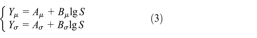
where the subscripts μ and σ are mean value and standard deviation of each parameter. By assuming that Y follows normal distribution, A_μ, B_μ, A_σ, and B_σ can be solved through maximum the likelihood function below ¹⁵

$$\begin{array}{c}\mathrm{InL}(A_{\mu },B_{\mu },A_{\sigma },B_{\sigma })=-\sum _{i=1}^n\hfill \\ \{\mathrm{In}\sqrt{2\pi }+\mathrm{In}(A\sigma +B\sigma \lg \mathrm{Si})+\frac{1}{2}{\left[\frac{\mathrm{Yi}-(A\mu +B\mu \lg \mathrm{Si})}{A\sigma +B\sigma \lg \mathrm{Si}}\right]}^2\}\hfill \end{array}$$

(4)

Then, the second part of the curve can be obtained by CPM. Based on first part parameters received previously, four key parameters of extrapolation can be obtained as

$$\lg N_T=\frac{A_{P-C}{B}_{\mu }-A_{\mu }{B}_{P-C}+B_{\mu }{B}_{P-C}(\lg S_{-1P-C}-\lg S_{-1\mu })}{B_{P-C}-B_{\mu }}$$

(5)

$$k_T=\frac{\lg N_{-1}-\lg N_T}{B_{\mu }(\lg S_{-1\mu }-\lg S_{T,\mu })}$$

(6)

$$G_{P-C}=\lg N_T-k_T{B}_{P-C}\lg S_{T,P-C}$$

(7)

$$H_{P-C}=k_T{B}_{P-C}$$

(8)

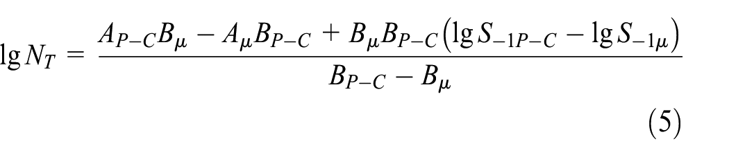
So that the curves can be expressed as

$$\{\begin{array}{c}{Y}_{P-C}=A_{P-C}+B_{P-C}\lg S(N⩽N_T)\hfill \\ \multicolumn{1}{c}{Y_{P-C}=G_{P-C}+H_{P-C}\lg S(N>N_T)}\end{array}$$

(9)

where N_T and k_T are transforming point and factor, respectively. S₋₁ is the fatigue limit of material, N₋₁ is fatigue life corresponding to fatigue limit, and S_T is the strength at transforming point. G and H are basic parameters of curves, P is survival probability and C denotes confidence coefficient. Subscript P–C indicates each value at arbitrary P–C levels.

In fact, strength is a function of life and should be time-varying, and the strength decreases due to the irreversible material degradation. Life distribution in this article is supposed to be a normal distribution. According to Murty et al., ³ life distribution PDF f(N|S) could be converted into strength distribution PDF f(S|N), and they would share the same distribution type. So that from PCSN curves, once life is specified, the strength distribution corresponding to the specific life can be derived from life distribution as ¹⁶

$$F(S_a,N_{\exp })=\mathrm{\Phi }\left(\frac{S_a-{\mu }_{s_a}}{{\sigma }_{s_a}}\right)$$

(10)

$$\begin{array}{c}{\mu }_{s_a}=K_{\mathrm{av}}{10}^{\frac{\lg N-A_{\mu }}{B_{\mu }}}[2-{10}^{\frac{-t_{1-C}(n-2)s_r\sqrt{1+1/n}}{B_{\mu }}}],\hfill \\ {\sigma }_{s_a}=K_{\mathrm{rms}}{10}^{\frac{\lg N-G_{\mu }}{H_{\mu }}}\hfill \end{array}$$

(11)

$$\begin{array}{c}{\mu }_{s_a}=K_{\mathrm{av}}{10}^{\frac{\lg N-G_{\mu }}{H_{\mu }}}[2-{10}^{\frac{-t_{1-C}(n-2)s_r\sqrt{1+1/n}}{H_{\mu }}}],\hfill \\ {\sigma }_{s_a}=K_{\mathrm{rms}}{10}^{\frac{\lg N-G_{\mu }}{H_{\mu }}}\hfill \end{array}$$

(12)

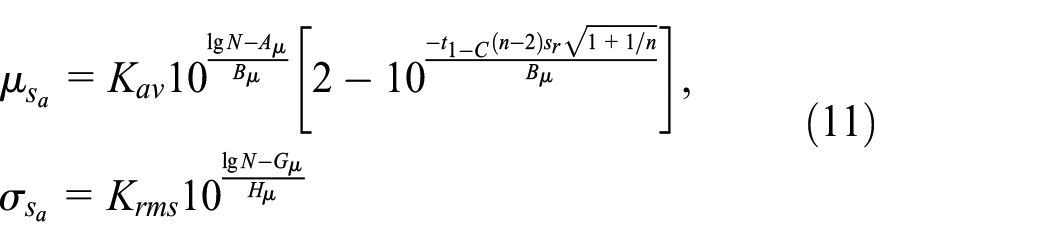
where K_av and K_rms are the mean value and standard deviation of structural fatigue modification factor, respectively. These values are used to consider scale factor and surface quality factor. μ_sa is the mean value of strength distribution and σ_sa is the standard deviation of strength distribution.

Multiaxial stress state and stress distribution

Figure 2 shows the process of obtaining the stress distribution. In Figure 2, MBD model is built to get vertical force history between wheel and rail while the measured history can also be used. Finite element model is employed to get the stress components history of elements in wheel critical part under a series of vertical force levels (5–8 levels). Since wheel is axial symmetry, it is supposed that the damage for elements with the same rolling diameter in a rolling cycle is identical. So that the wheel critical part can be defined to be the stress concentrate area of any circumferential cross section of wheel. Given that the wheel is always under multiaxial stress state during rolling contact with rail, after obtaining critical part elements’ stress components history in a rolling cycle under different vertical force levels, multiaxial equivalent stress of these elements would be determined.

Figure 2.

Schematic diagram of process of obtaining stress distribution.

A lot of multiaxial fatigue model have been proposed to calculate a multiaxial equivalent stress based on stress components, such as Findley, ¹⁷ McDiarmid, ¹⁸ Liu, ¹⁹ and Carpinteri–Spangnoli (C-S). ²⁰ Each of them can be employed to calculate the equivalent stress. However, according to Gonçalves et al., ²¹ C-S model is used in this article. Equation (13) gives the equivalent stress expression in C-S model

$$\begin{array}{c}{\sigma }_{a,\mathrm{eq}}=\sqrt{N_{a,\mathrm{eq}}^2+{\left(\frac{{\sigma }_f}{{\tau }_f}\right)}^2{C}_a^2}={\sigma }_f\hfill \\ N_{a,\mathrm{eq}}=N_a+{\sigma }_{-1}\left(\frac{N_m}{{\sigma }_u}\right)\hfill \end{array}$$

(13)

where σ_a, _eq is the multiaxial equivalent stress amplitude, and N_a, N_m, and C_a are normal stress amplitude, normal stress mean value, and shear stress amplitude on the critical plane, respectively. σ_f and τ_f are material fatigue limit of uniaxial test and torsion test under f load cycles, respectively. σ_u is the material tension strength. Details about the process to determine the critical plane can be found in Carpinteri et al. ²⁰ By trail-and-error method, set initial value f = 5E6, and after some iterations, the left side would be equal to the right side, and σ_a, _eq is determined.

How to convert the force history between rail and wheel into the stress history of a wheel element efficiently is a key problem in this article. To solve this problem, it is assumed that there is a relationship between the vertical force and the multiaxial equivalent stress. So that after obtaining each critical part element’s multiaxial equivalent stress under different vertical force levels, the relationship between force and stress of each element can be fitted as equation (14)

$${\sigma }_{a,\mathrm{eq}}=a{F}^n+b{F}^{n-1}+\cdots +\mathrm{cF}+d$$

(14)

where F is the vertical force between wheel and rail.

Because only straight track is considered and wheelset lateral displacement is ignored, after obtaining each critical part element’s force–stress relationship, the one with the highest equivalent stress level is used to convert the force history into the stress history. The stress distribution can be received by distribution fitting of the stress history. Finally, the reliability can be assessed by stress–strength interference theory.

Results and discussion

In order to verify the method proposed in section “Material and methods,” a case study will be shown in this section. The reliability assessment of the CRH5 train wheel will be performed as follows.

Strength distribution

The material of CRH5 wheel is R8T-type steel, and the mechanical properties of R8T are listed in Table 1.

Table 1.

Mechanical properties of R8T.

Material	Fatigue limit (MPa)	Yield strength (MPa)	Tensile strength (MPa)
R8T	343	647	910

Figure 3(a) shows the hydraulic servo tension and compression fatigue machine. Its maximum load value and load frequency are 100 kN and 50 Hz, respectively. The shape and size of R8T specimen for fatigue tests are shown in Figure 3(b) with its maximum and minimum diameters 16 and 8 mm, respectively.

Figure 3.

Fatigue machine with environmental chamber and specimen: (a) Fatigue machine and (b) test specimen.

To determine the fatigue limit of R8T, an up-and-down test is carried out. In this article, the number of cycles which regarded as “runout” is 5E6 cycles, and the results are shown in Figure 4. Totally, 15 specimens are tested, and 14 of them are divided into seven pairs to calculate the fatigue limit.

Figure 4.

Up-and-down test results of R8T.

Fatigue tests are carried out under a symmetrical loading, seven different stress levels are selected, 19 specimens are tested in total, and the results are displayed in Figure 5(a). In Figure 5(a), abscissa axis is lifetime cycle and axis of ordinate is stress amplitude. As we can see from the picture, the life of specimen express distinct randomness under same stress level as its difference can be up to 100 times. To describe this randomness exactly, PCSN curves instead of an S-N curve are needed. Figure 5(b) shows the failure sample in the fatigue test.

Figure 5.

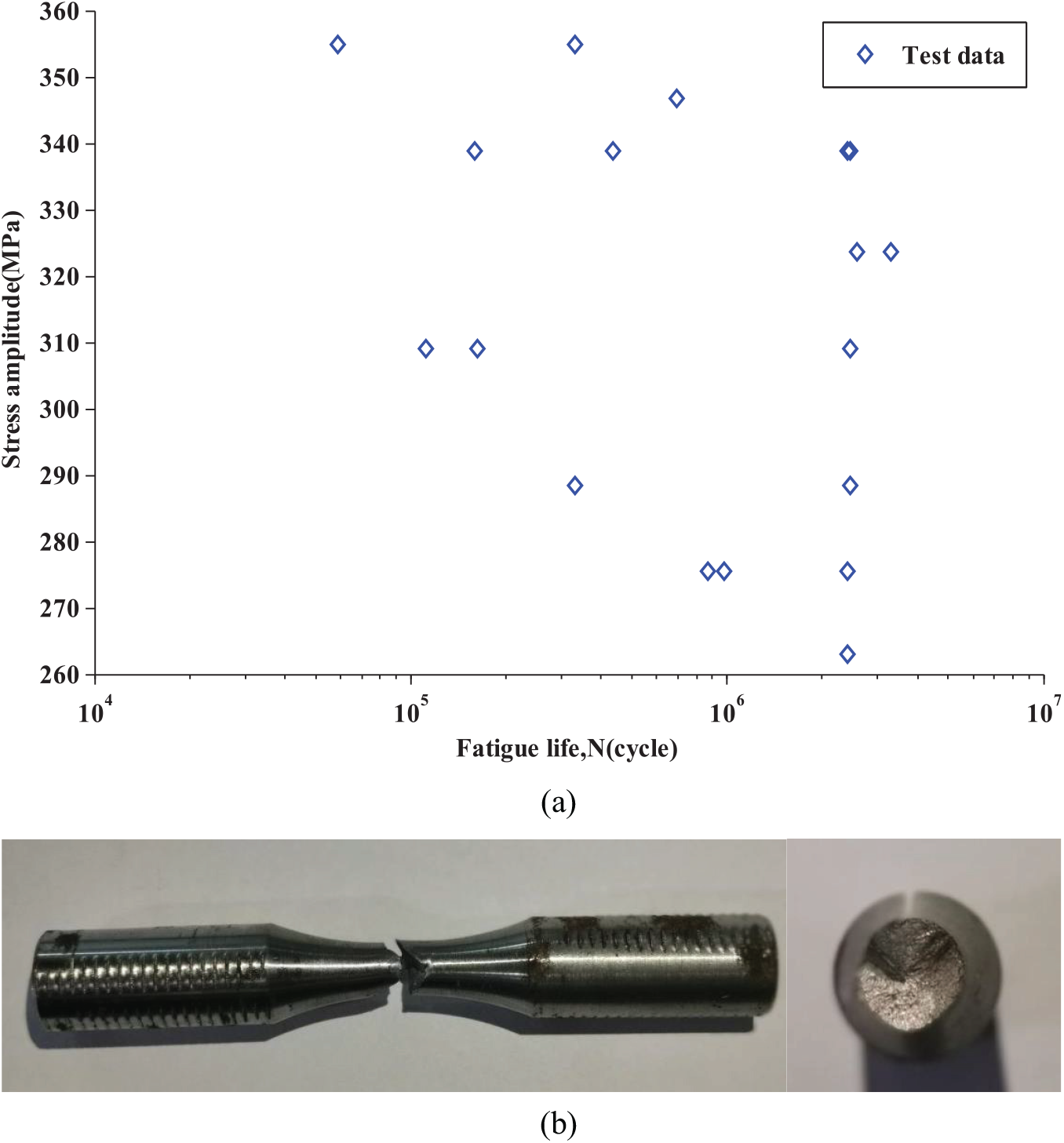
Fatigue test result of R8T: (a) stress–life results and (b) failure sample.

The basic parameters of PCSN curves are computed and listed in Table 2. s_r is residual standard deviation and the calculation method of s_r can be referred to Zhao et al.’s ²² work.

Table 2.

Basic parameters of PCSN curves of R8T.

Aμ	Bμ	Aσ	Bσ	sr	NT	kT
20.21	−5.58	1.25	−0.28	0.537	627,769	3.446

PCSN: probabilistic confidence stress life.

Meanwhile, parameters of PCSN curves at different P–C levels are listed in Table 3.

Table 3.

Parameters of PCSN curves at different P–C levels.

		A	B	G	H
C = 50%	P = 50%	20.21	−5.58	55.46	−19.23
	P = 90%	18.61	−5.22	49.95	−17.99
	P = 99%	17.30	−4.93	45.43	−16.99
C = 90%	P = 50%	19.48	−5.58	52.95	−19.23
	P = 90%	17.88	−5.22	47.43	−17.99
	P = 99%	16.58	−4.93	42.95	−16.99
C = 99%	P = 50%	18.80	−5.58	50.60	−19.23
	P = 90%	17.19	−5.22	45.06	−17.99
	P = 99%	15.89	−4.93	40.58	−16.99

PCSN: probabilistic confidence stress life.

Using the parameters obtained above, the results of strength distribution PDF with different expectation lives are listed in Table 4. In this article, K_av = 0.86 and K_rms = 0.034. ⁷ As we expected, the mean value of strength decreases as fatigue life increases.

Table 4.

Structure strength PDF parameters with different confidences and lives.

C	N cycles	μ (MPa)	σ (MPa)
50%	5E6	295	11.67
	1E7	285	11.26
	5E7	262	10.36
	1E8	253	10
	5E8	232	9.2

Stress distribution

Dynamic simulation was conducted in Simpack 9.6. Simpack is a professional MBD simulation software with a powerful railway module. The dynamic model consists of a vehicle body, two bogies, four wheel pairs, and primary as well as secondary suspensions. Primary suspensions connect body with bogies and secondary suspensions link bogies with wheel pairs. Generally, there are three types of working conditions during operation including straight, curve, and turnout. Here, only the straight condition was applied to build a track model considering the fact that most of the high-speed railway track geometry is straight. In order to include the irregularity of railway track during operation, this article adds irregularity spectrum to the model including vertical, lateral, and gauge irregularities. Set the running speed according to the working condition, and the vertical force between rail and wheel can be obtained.

The length, width, and height of a power coach of CRH5 vehicle were 25,000; 3200; and 4270 mm, respectively. The tread type of its wheel is XP55. The total length of track is 5 km and gauge is 1435 mm. The wheel rolling diameter is 890 mm. The running speed is 200 km/h. Other parameters are shown in Table 5.

Table 5.

Basic parameters of dynamic model.

Name	Value	Unit
Body mass	43,600	kg
Bogie mass	4760	kg
Wheel pair mass	1800/1500	kg
Body moment of inertia x	100,500	kg m2
Body moment of inertia y	1,223,000	kg m2
Body moment of inertia z	1,296,000	kg m2
Bogie moment of inertia x	1800	kg m2
Bogie moment of inertia y	8000	kg m2
Bogie moment of inertia z	9000	kg m2
Wheel pair moment of inertia x	1263/1000	kg m2
Wheel pair moment of inertia y	210/150	kg m2
Wheel pair moment of inertia z	1285/1000	kg m2
Primary suspension vertical stiffness	2.3996	MN/m
Secondary suspension vertical stiffness	0.8858	MN/m
Primary suspension vertical damping	30	kN s/m
Secondary suspension vertical damping	45	kN s/m

The vertical force history between rail and wheel is shown in Figure 6. As the lateral force is small enough to neglect in a straight track, only the vertical force is considered. It seems that vertical force between wheel and rail is in the range of 68,000–78,000 N.

Figure 6.

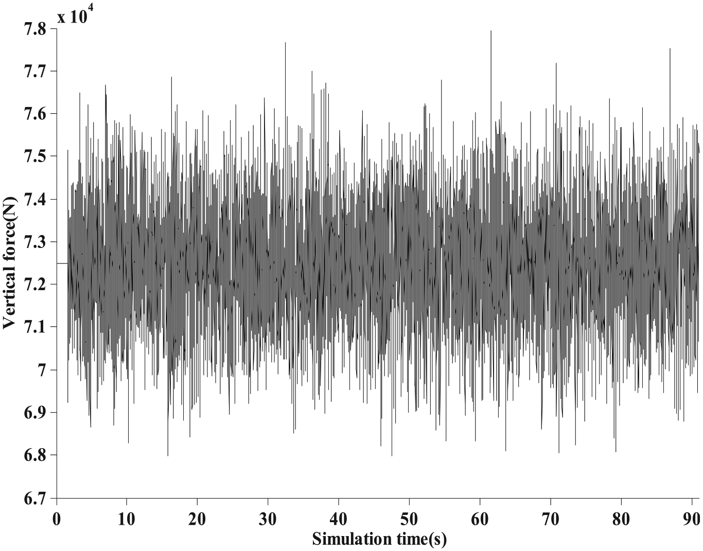
Simulated vertical force history.

Based on the vertical force result, five different levels of vertical force including 50,000; 60,000; 70,000; 80,000; and 90,000 N were used in the finite element analysis. A bilinear elasto-plastic material model is used to build the finite element model in ABAQUS with 250,000 elements as well as 480,000 nodes in total (Figure 7(a)–(c)). Elements’ size in potential contact area were refined to 0.8 × 0.8 mm²; Zhao and Li ²³ studied the mesh size effect on simulation results and found that a size smaller than 1.3 × 1.3 mm² could guarantee the accuracy of results. Element type was C3D8I for avoiding the hourglass problem. The loading position was in consistent with UIC510-5 standard. ²⁴ A reference node was set up on the wheel axis in order to couple it with wheel hole surface to control the wheel degrees of freedom. The bottom surface of the rail was fixed. The initial contact patch center is set as the origin of coordinates (Figure 7(d) and (e)). The running direction of wheel was longitudinal along the z-axis. The axial direction of the wheel was lateral along the y-axis and vertical along the x-axis. The simulation contained two steps: in the first step, vertical force was loaded and contact between wheel and rail was set up. Then, in the second step, angular velocity was added to the wheel and the wheel would move forward. Figure 7(f) shows the von Mises stress result of wheel–rail contact under 90,000 N vertical force, and the maximum stress is 815 MPa.

Figure 7.

FE model and von Mises stress result: (a) FE model, (b) Wheel material model, (c) Rail material model, (d, e) Coordinates of the model, and (f) von Mises stress result.

The results of stress state of an element under wheel tread are shown in Figure 8. The vertical force was 90,000 N. The picture expresses a whole process that the element approaches and leaves the contact patch between wheel and rail. Obviously, the wheel is under multiaxial stress state from Figure 8. The stress components of each element in the critical part of wheel would be used to calculate its multiaxial equivalent stress.

Figure 8.

Stress state of an element under wheel tread.

The multiaxial equivalent stress under different vertical forces could be calculated by the C-S model (equation (13)). Fatigue limit under different load cycles could be determined based on the mean value tension–compression S-N curve obtained from section “Strength distribution,” and the mean value torsion S-N curve in Cai. ¹⁶ The two curves are shown in Figure 9.

Figure 9.

Mean value S-N curves of wheel.

Then, the force–stress relationship of CRH5 wheel is obtained by polynomial fitting. By comparing force–stress relationship of each element in critical part, the relationship of element No. 678000092 (x = −2 mm, y = 2 mm, z = 72 mm) is used, and the element position is shown in Figure 10. The relationship result is plotted in Figure 11.

Figure 10.

Element position in the model.

Figure 11.

Force–stress relationship of CRH5 wheel.

Apply the relationship to convert the vertical force history into stress history and fit the stress distribution. The fitting result in Figure 12 shows that the stress follows normal distribution with μ = 267 MPa, σ = 6.7 MPa.

Figure 12.

Stress distribution of the wheel critical part.

Reliability of CRH5 wheel

When stress and strength distributions have been obtained, a reliability assessment could be fulfilled by stress–strength interference as

$$R(N_{\exp },C)=\underset{0}{\overset{+\infty }{\int }}f(S_a,N_{\exp },C)\underset{0}{\overset{S_{-1}}{\int }}({\sigma }_{-1a},C)d{\sigma }_{-1a}d{S}_a$$

(15)

If they all follow normal distribution

$$R(N_{\exp },C)=\mathrm{\Phi }\left(\frac{{\mu }_{s_a}-{\mu }_{{\sigma }_{-1a}}}{\sqrt{{\sigma }_{s_a}^2+{\sigma }_{{\sigma }_{-1a}}^2}}\right)$$

(16)

To verify the method proposed, first, the crack initiation life result at P = 50%, C = 50% is compared with other studies. For example, in Liu et al. ²⁵ and Zhang, ²⁶ they are 32,000 and 70,000 km, respectively. They are similar as the result in this article which is 97,000 km, although there are some differences in the input parameters.

The reliability assessment results are shown in Table 6. As the life increases, the reliability decreases. The design life of CRH5 wheel is more than 600,000 km; however, according to the results from Table 6, with 50% confidence, the reliability of wheel corresponding to 280,000 km mileage is only 12.2%. That means there will be crack initiation and growth around the area 2 mm under the tread early during operation. If the crack propagates without wheel maintenance, it will lead to fatigue failure quickly on early stage of operation.

Table 6.

Reliability assessment results of wheel.

C	N cycles	Mileage (km)	R
50%	5E6	1.4E4	98.2%
	1E7	2.8E4	91.5%
	5E7	1.4E5	34.2%
	1E8	2.8E5	12.2%
	5E8	1.4E6	0.11%

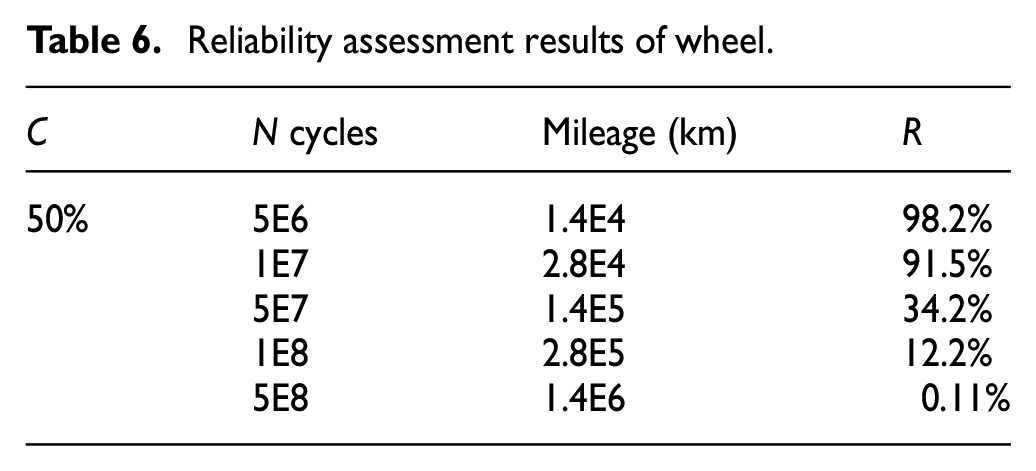
Figure 13 shows the relationship between reliability and life with speed at 200 km/h. As we can see from the picture, each line follows similar tendency including three phases, which is reliability keeps stable at the beginning, then decreases rapidly at the middle, and declines slowly at the end of the line with the life increases.

Figure 13.

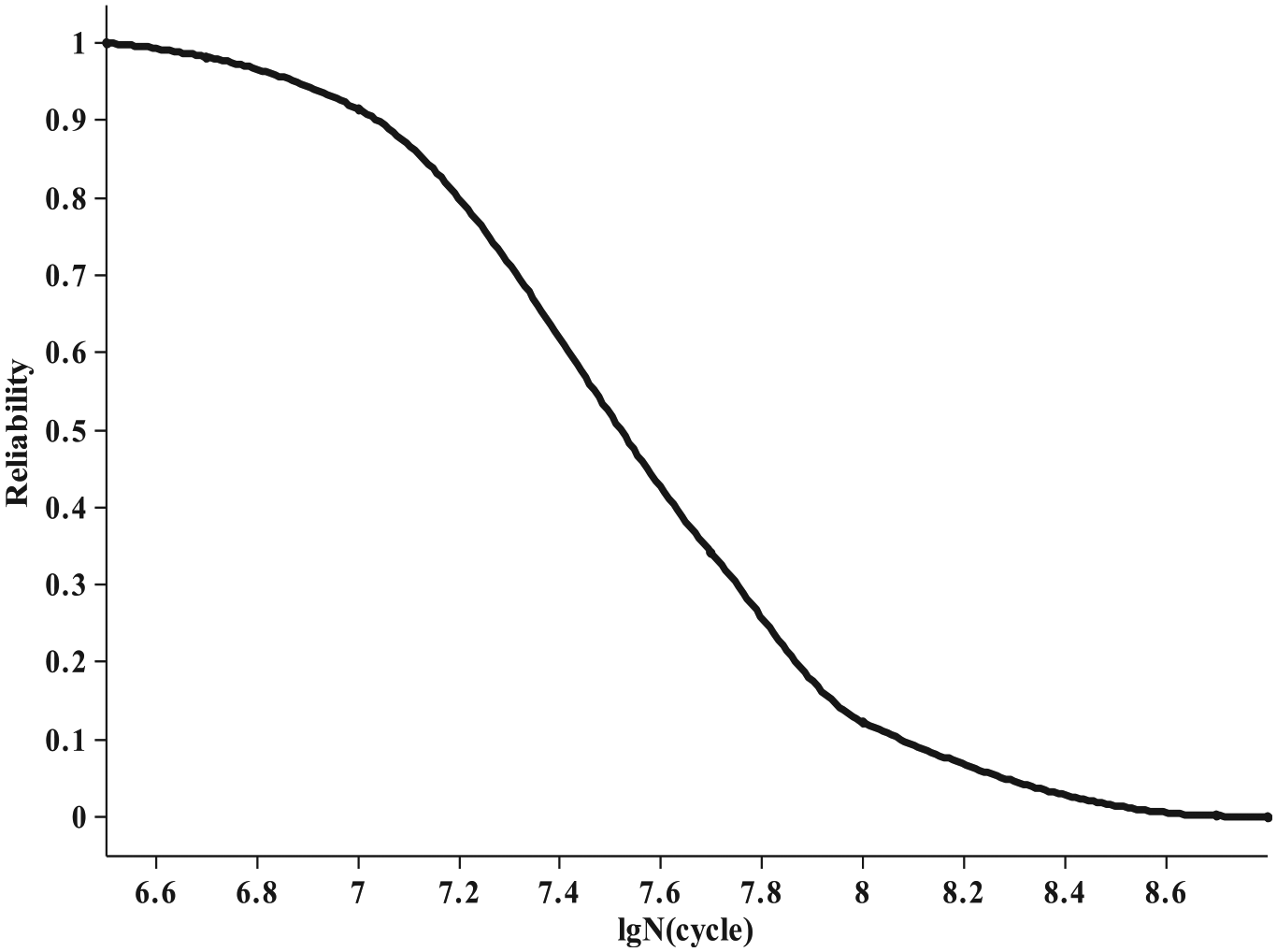
Reliability verses life cycles.

According to Zhang, ²⁶ the mileage for the first-time complete overhaul of CRH5 wheel is 120,000 km, that means its fatigue reliability is about 35%. Actually, it is relatively low and probably explained by the following reasons:

1. This article sets the speed value of train at 200 km/h, which is the highest speed during operation; however, the train would not keep running at the highest speed in fact. So that the effect of speed on fatigue reliability would be studied as follows.

Considering the actual operation situation, four speed levels besides 200 km/h are selected including 100, 125, 150, and 175 km/h. Apply the same procedure in section “Material and methods” to obtain the stress distribution PDF at different speeds as shown in Table 7. Similarly, they all follow normal distribution.

Table 7.

Stress distribution PDF at different speeds.

Speed (km/h)	μ (MPa)	σ (MPa)
100	234	4.7
125	246	5.2
150	255	5.3
175	263	6.2

Reliability at different speed levels under 50% confidence are shown in Figure 14. From the picture, we find that with the same life cycles, the higher the speed, the lower the reliability. At the beginning, the four lines show no difference, then in high-cycle fatigue region, the difference starts to increase until life reaches about 1E9 cycles. The reliability at 100 km/h can be as large as nine times of that at 200 km/h under the same lifetime, that means speed is a key factor in reliability assessment and it should be more cautious for railway speed increasing:

• 2. In the fatigue reliability assessment process, only crack initiation life is considered while the crack propagating life is neglected. In fact, after crack initiation, it still needs time for it to propagate. While during this time period, the wheel could work as usual. The reliability would rise after considering the crack propagating life.

• 3. In this article, the lateral position of wheel rail contact is constant during simulation and lateral displacement is not included. In fact, due to track geometry and irregularity, the lateral position of wheel rail contact is changing every time, and this could extend the contact area and reduce damage, as a result, to increase the fatigue life and reliability of wheel.

As for the limitations of this study: first, only crack initiation life is considered in the study, the process for crack propagation is ignored; second, no lateral displacement between wheel and rail is included. All of the two points will be considered in the future study.

Figure 14.

Reliability at different speed levels.

Conclusion

This article proposed an efficient fatigue reliability assessment method and assessed the fatigue reliability of CRH5 wheel, and the following conclusions can be drawn:

1. The proposed method can assess the fatigue reliability of wheel efficiently based on the measured force history between wheel and rail.

2. With 50% confidence, the reliability of wheel corresponding to 280,000 km mileage is only 12.2%. That means there will be crack initiation and growth around the point 2 mm under the tread early during operation. If the crack propagates without wheel maintenance, it will lead to fatigue failure quickly.

3. As lifetime increases, the wheel reliability changes in three phases: stable phase at the beginning, rapidly decrease phase in the middle, and slowly decline phase at the end of the line; Speed is a key factor in reliability assessment, the higher the speed, the lower the reliability.