Sage Journals: Discover world-class research

Abstract

Pedestrian simulation modeling has become an important means to study the dynamic characters of dense populations. In the continuous pedestrian simulation model for complex simulation scenario with obstacles, the pedestrian path planning algorithm is an indispensable component, which is used for the calculation of pedestrian macro path and microscopic movement desired direction. However, there is less efficiency and poor robustness in the existing pedestrian path planning algorithm. To address this issue, we propose a new pedestrian path planning algorithm to solve these problems in this article. In our algorithm, we have two steps to determine pedestrian movement path, that is, the discrete potential fields are first generated by the flood fill algorithm and then the pedestrian desired speeds are determined along the negative gradient direction in the discrete potential field. Combined with the social force model, the proposed algorithm is applied in a corridor, a simple scene, and a complex scene, respectively, to verify its effectiveness and efficiency. The results demonstrate that the proposed pedestrian path planning algorithm in this article can greatly improve the computational efficiency of the continuous pedestrian simulation model, strengthen the robustness of application in complex scenes.

Keywords

Algorithm path planning potential field pedestrian simulation transportation

Introduction

With the development of economy, people communicate with each other frequently and there are more and more crowds of people in large public places such as airports, railway stations, supermarkets, gymnasia, and theaters. Dense crowds have the potential to become impenetrable or to develop into an unsteady state with turbulent flows,^1–4 which are likely to compromise individual safety. In many instances, fatalities and injuries are not caused by exogenous factors such as fire, explosions, poisonous gas, or other hazards, but by crowd behavior itself. Therefore, pedestrian mobility behavior has gradually attracted the attention of scholars. Many pedestrian simulation models have been proposed to study the characteristics of pedestrian behavioral, movement laws, and evacuation.^5–11 To simulate crowds in large and complex environment, individuals need to behave realistically both at a local level as well as at a global level when navigating the environment, that is, the pedestrian simulation can be regarded as a process that combines local motion planning with global path planning, corresponding to the microscopic motion model and the macroscopic path planning model. The microscopic motion models, such as the social forces model^5–7 and the cellular automata model,^8–11 consider the movements of each individual and focus on the interaction between individuals in local minima. The macroscopic path planning model has been proposed to deal with the crowd navigation at a global scale and derive the pedestrian desired speed direction for the microscopic motion model.

The crowd navigation can be modeled using network graph models. This class of models involves two aspects: spatial map generation and path planning algorithm. The spatial map, which is often made up of a series of nodes and edges, can capture many structural properties as well as the topological relationship of spatial arrangement. According to the spatial map, the path planning algorithm can obtain a proper route which consists of a series of nodes. Then, the pedestrian can move by the desired speed direction which directs from the current position to the adjacent node along the route. Therefore, crowd navigation functions as a guide of the pedestrian’s local movement. If the target or the destination changes during the motion, the individual has to employ the macroscopic path planning model to plan the path from the current position to the new destination, making the individual change the desired speed direction.

As to the spatial map representation modeling, the visibility graph,^12–14 the Voronoi diagram,^15–20 and the navigation mesh^21–24 serve as the widely used map generation modeling method. In the visibility graph, the initial position, the goal position, and the vertices of obstacles in the simulation scenario are represented by the nodes. The walkable areas represent edges which act as a connector between the nodes. Kneidl et al.²⁵ presents an advanced method for the automated generation of a visibility graph to model large-scale way-finding decision. Based on the visibility graph, Kneidl et al.¹² has given a hybrid multi-scale model which combined with a large-scale navigation method and a small-scale navigation method for simulation of pedestrian dynamics. Turner et al.¹³ presented a method to generate a graph of mutual visibility between locations based on a set of isovists, and their works showed that the visibility graph properties can predict pedestrians’ spatial behavior and simulate the way-finding process. Wang et al.¹⁴ developed a space visibility graph model with cognitive pedestrian behavior and individual characteristics to analyze the pedestrian’s navigation decision and movement patterns.

The Voronoi diagram method divides the region into sub-regions with polygons which encircle the obstacles. Unlike the visibility graph, the nodes of the spatial map are the vertices of polygons, and the edges of the map are the sides of polygons constructed using equidistant points from the adjacent two points on the obstacle’s boundaries. Kambara et al.¹⁵ applied the concept to construct a Delaunay diagram from neighbor nodes in the Voronoi diagram and used network Voronoi diagram to construct a subgraph based on the context for pedestrian route search. Nakamura et al.¹⁶ has given a pedestrian movement model based on the Voronoi diagram, by which the walking route and direction of each pedestrian can be determined. Xiao et al.¹⁷ introduced Voronoi diagram to obtain some useful motion information of pedestrian dynamic, such as local density, safe distance, and neighbors. And the walking direction of pedestrian in Voronoi cell can be divided into destination direction, potential detour direction, and potential following direction.¹⁸ The three elementary walking directions are calculated inspired by the characteristics of the shapes of Voronoi cell. Šeda and Pich¹⁹ have shown that generalized Voronoi diagrams can be used for fast generation of smooth paths sufficiently distant from obstacles. Hiyoshi et al.²⁰ proposed a Voronoi cellular automaton model using the Voronoi diagram as the underlying mesh to reproduce phenomena about walking direction decision which comes from the local features, such as corners.

As similar to the Voronoi diagram, the navigation mesh also divides the region into sub-regions with convex polygons. The navigation mesh can be categorized into triangulation and polygonization according to the number of sides of polygons. The adjacencies of these convex regions of open space are then calculated and used to construct a graph of connectivity between convex regions. Each region is a node on the graph and if two regions share a common edge in space, they are connected by an edge. Xia et al.²¹ employed the triangular meshes to solve the reactive dynamic user equilibrium model for pedestrian flows based on a discontinuous Galerkin method. Boguslawski et al.²² proposed a novel automated construction of navigation mesh by considering the variability of pedestrian density on the route, and derived a variable density navigation network for determining egress paths in the pedestrian evacuation. Chen et al.²³ presented a computation model on the general triangular grid and studied the modeling of pedestrian dynamics on triangular grids.

Navigation process with network graph models is usually considered as an optimization problem of route decision. In these optimization problems, the numbers of pedestrians in these nodes are seen as the decision variables. However, the efficiency issues of computation must be considered before applying this class of models to navigation. The algorithms for generating network is relatively complex that may result in low computational efficiency. Even more, they were insufficient robustness in the complex simulation scenarios. For instance, it should be recalculated when the scene environment changes, such as the fire smoke that is dynamically diffused. The efficiency of the navigation graph algorithm is $O (n \log n)$ ²⁴ that may result in low computational efficiency when the simulation scale and the number of the pedestrian increase.

At present, potential field method has been widely used in mobile path planning, such as robots, vehicle, and pedestrian.^26–28 In the potential field method, the simulation space is divided into a set of uniform grids called as cells. Each grid has been assigned a potential field value which can reflect the utility cost such as distance, congestion, discomfort cost, and the influence of other pedestrians.^29–33 A gradient can therefore be applied based on the potential field that guides the agents from the source to the destination. These methods are useful to reduce the complexity at a macroscopic level.

Therefore, to avoid the less efficiency and poor robustness in the existing pedestrian path planning algorithm, we propose a new pedestrian path planning algorithm based on the potential field model in this article. Meanwhile, considering the computational efficiency of the potential field for navigation, this article draws on the idea of discrete potential field, proposes a calculation method of potential field, and then obtains the pedestrian’s desired speed direction in the pedestrian simulation model, which can realize the pedestrian movement path planning in complex scenes.

The rest of this article is organized as follows. Section ‘Algorithm and model description’ presents an algorithm to calculate the potential field by considering the distance, and then the pedestrian desired speed direction can be obtained for route navigation on the basis of the discrete potential fields. Section ‘Numerical results’ analyzes the property and applicability of the proposed method of route navigation based on grid potential field, both in the simple scenes and complex scenes. Finally, concluding remarks and future research directions are given in section ‘Conclusion’.

Algorithm and model description

In this section, the desired speed direction is calculated by two steps. The first step is to generate a discrete potential field by the flood fill algorithm,³⁴ and then the pedestrian desired speed direction is determined along the negative gradient direction in the discrete potential field.

Algorithm for grid potential field

In the flood filling method-based algorithm for generating the grid potential field, the two-dimensional (2D) square grid is first used to convert the continuous space into a grid system with the grid unit size represented as $μ$ . The grids are divided into four types according to the simulation layout, that is, blank grids, girds occupied by walls, grids occupied by obstacles, and exit grids, where the blank grids and exit grids can be used for pedestrian movement. The size of the grid system and the type of each grid can be determined according to the coordinate parameters of walls, obstacles, exits in the continuous space scene. Then, their neighborhood is given by extended Moore neighborhood, namely the neighborhood set of the grid $(x, y)$ is $F_{(x, y)}^{w} = {(i, j) | | i - x | \leq w, | j - y | \leq w}$ , where $w$ is the range parameter of neighborhood. When $w = 1$ , it is the Moore neighborhood.

The detailed algorithm for generating the potential field of the grids is as follows.

Step 1. Initialization. The temporary potential field $st (x, y)$ of wall grids, obstacle grids, blank grids are set as $st (x, y) = + \infty$ , and the temporary potential field $st (x, y)$ of exit grids are set as $st (x, y) = 0$ . Meanwhile, the exit grids are added into set A.

Step 2.1. Select the grid $(x, y)$ with the minimum value of $st (x, y)$ in set A, and traversing the blank grids $(i, j) \in F_{(x, y)}^{1}$ . If $| i - x | + | j - y | = 1$ and $st (i, j) > st (x, y) + 1$ , we have $st (i, j) \leftarrow st (x, y) + 1$ . If $| i - x | + | j - y | = 2$ and $st (i, j) > st (x, y) + \sqrt{2}$ , we have $st (i, j) \leftarrow st (x, y) + \sqrt{2}$ . Then the grid $(i, j)$ is added into set A. We loop all the blank grids $(i, j) \in F_{(x, y)}^{1}$ and remove this type of grid $(x, y)$ from set A.

Step 2.2. If $A \neq \emptyset$ , go to Step 2.1, otherwise go to Step 3.1.

Step 3.1. Constructing an empty sequence $SE 1$ . Traversing all the blank grids in the system. For the blank grid $(i, j)$ , if the value of $st (i, j)$ is not in sequence $SE 1$ , adding this value into sequence $SE 1$ in ascending order.

Step 3.2. Construct an arithmetic progression $SE 2$ . The number of items in sequence $SE 2$ is the same as that in sequence $SE 1$ , and we set it as N. Then, we set the first element of $SE 2$ as $a_{1} = 0.1$ and the last element as $a_{N} = 1.0$ , respectively. While it is $a_{n} = a_{1} + (a_{N} - a_{1}) (n - 1) / (N - 1)$ for the nth element in $SE 2$ .

Step 3.3. Traversing all the blank grids in the system. For the blank grid $(i, j)$ , we set its potential field $s (i, j)$ as $a_{n}$ , where $n$ is determined by the location of $st (i, j)$ in $SE 1$ .

Step 4. Traversing all the obstacle grids in the system. For the obstacle grid $(x, y)$ , we have $s (x, y) = \max {s (i, j) | s (i, j) \in F_{(x, y)}^{1}}$ .

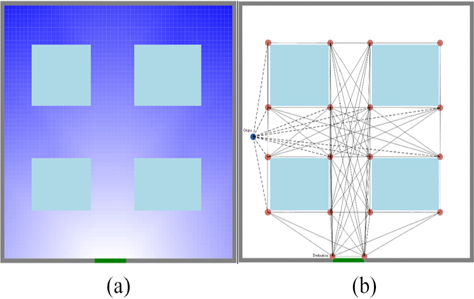
Figure 1 illustrates the potential field in a room with obstacles, where Figure 1(a) shows a continuous space scene, where the red line indicates the wall, the blue line indicates the obstacle, and the green line indicates the exit; Figure 1(b) shows discrete grid scenes, gray grids are wall or obstacle, green grids are exit, and the rest are blank grids. When the range parameter of neighborhood $w = 1$ , the temporary potential field $st (x, y)$ and potential field $s (x, y)$ of grid $(x, y)$ are shown in Figure 1(b) and (c), respectively.

Figure 1.

Illustration of discretization scene and potential field calculation: (a) the continuous space scene, (b) the temporary potential field in discrete grid scene, and (c) the potential field in discrete grid scene.

Calculation of pedestrian speed desired direction

As mentioned above, the process of route navigation for a pedestrian is actually to calculate the pedestrian’s speed desired direction in the potential field method. In this article, the speed desired direction is determined by the negative gradient direction in the grid potential field. The concrete calculating method is as follows.

For the pedestrian locating at $\vec{l} = (x_{l}, y_{l})$ in the continuous spatial coordinate system, we assume that the pedestrian seated in grid $(x, y)$ in the discrete grid system, where $x = x_{l} / μ + 1$ , $y = y_{l} / μ + 1$ . Set the $(x_{0}, y_{0})$ and $(x_{i}, y_{i})$ as center points of the grid $(x, y)$ and the grid $(i, j)$ , respectively, in continuous spatial coordinate system, where $(i, j) \in F_{(x, y)}^{w}$ . The negative gradient direction $P$ of grid $(x, y)$ is

P = {(\begin{matrix} \sum_{(i, j) \in F_{(x, y)}^{w}} (s (i, j) - s (x, y)) (x_{i} - x_{0}) \\ \sum_{(i, j) \in F_{(x, y)}^{w}} (s (i, j) - s (x, y)) (y_{i} - y_{0}) \end{matrix})}^{T}

(1)

We set the speed desired direction of the pedestrian ${\vec{e}}_{(x, y)}^{1}$ in grid $(x, y)$ as the unit vector along the negative gradient direction of grid $(x, y)$ . Therefore, for the pedestrian located in the grid $(x, y)$ , we have

{\vec{e}}_{(x, y)}^{1} = \frac{P}{‖ P ‖}

(2)

In this section, we intend to verify the accuracy of our proposed method for pedestrian speed desired direction through comparative analysis with other two different methods in the existing literature. Guo and Huang³⁵ proposed an algorithm for the static potential field (hereinafter referred to as Guo’s potential field) and their formulation for pedestrian speed desired direction (hereinafter referred to as ${\vec{e}}_{(x, y)}^{2}$ ) are as follows

{\vec{e}}_{(x, y)}^{2} = \frac{{(AB)}^{T}}{‖ {(AB)}^{T} ‖}

(3)

where $A = (\begin{matrix} \sum_{(i, j) \in F_{(x, y)}^{w}} ψ_{(i, j)} {(y_{i} - y_{0})}^{2} & - \sum_{(i, j) \in F_{(x, y)}^{w}} ψ_{(i, j)} (x_{i} - x_{0}) (y_{i} - y_{0}) \\ - \sum_{(i, j) \in F_{(x, y)}^{w}} ψ_{(i, j)} (x_{i} - x_{0}) (y_{i} - y_{0}) & \sum_{(i, j) \in F_{(x, y)}^{w}} ψ_{(i, j)} {(x_{i} - x_{0})}^{2} \end{matrix}),$ $B = (\begin{matrix} \sum_{(i, j) \in F_{(x, y)}^{w}} ψ_{(i, j)} (s (i, j) - s (x, y)) (x_{i} - x_{0}) \\ \sum_{(i, j) \in F_{(x, y)}^{w}} ψ_{(i, j)} (s (i, j) - s (x, y)) (y_{i} - y_{0}) \end{matrix})$ . In equation (3), if the grid $(x, y)$ is an obstacle grid, we set $ψ_{(i, j)} = 0$ . Otherwise, we set $ψ_{(i, j)} = 1$ .

The other one is proposed by Sun and Shi,³⁶ where they assumed that pedestrian preferred to move toward the grid with a smaller potential field and the pedestrian speed desired direction are mentioned as ${\vec{e}}_{(x, y)}^{3}$ in the following content, which is calculated by the following equation as

{\vec{e}}_{(x, y)}^{3} = \frac{C}{‖ C ‖}

(4)

where $C = {(\begin{matrix} p - x \\ q - y \end{matrix})}^{T}$ , $(p, q) = \arg {\min_{(i, j) \in F_{(x, y)}^{w}} {s (i, j)}}$ .

Actually, the speed desired direction in this article is an approximation of the desired direction calculating in continuous space according to equations (1) and (2). With the aim to analyze the deviation of the speed desired direction by potential field in the discrete grid from that in continuous space, we assume that the pedestrian is located at $(x_{0}, y_{0})$ in continuous space, which is the center point of the grid $(x, y)$ . As shown in Figure 2, according to the characteristic of pedestrian movement, the pedestrian always walks along the shortest path to the nearest point of the target area, such as corridor and exit. Therefore, we define the speed desired direction of pedestrian (hereinafter referred to as the original direction) located at $(x_{0}, y_{0})$ as

{\vec{e}}_{(x, y)}^{0} = \frac{{\vec{l}}_{(x, y)} - {\vec{c}}_{s}}{‖ ({\vec{l}}_{(x, y)} - {\vec{c}}_{s}) ‖}

(5)

where ${\vec{l}}_{(x, y)} = (x_{0}, y_{0})$ , ${\vec{c}}_{s}$ is coordinate of the nearest point of the target area in the 2D coordinate system.

Figure 2.

The pedestrian’s desire direction point to the nearest point of exit.

Set ${\vec{e}}_{(x, y)}^{0}$ as the reference vector, and $〈 {\vec{e}}_{(x, y)}^{0}, {\vec{e}}_{(x, y)}^{i} 〉$ denotes the angle between ${\vec{e}}_{(x, y)}^{0}$ and ${\vec{e}}_{(x, y)}^{i} (i = 1, 2, 3)$ , corresponding to equations (2)–(4). Furthermore, we calculate the cosine value $\cos 〈 {\vec{e}}_{(x, y)}^{0}, {\vec{e}}_{(x, y)}^{i} 〉$ to measure the deviation of the desired speed direction based on ${\vec{e}}_{(x, y)}^{i}$ from that based on ${\vec{e}}_{(x, y)}^{0}$ of grid $(x, y)$ . Obviously, $\cos 〈 {\vec{e}}_{(x, y)}^{0}, {\vec{e}}_{(x, y)}^{i} 〉$ is greater, ${\vec{e}}_{(x, y)}^{i}$ is closer to the original direction, which causes smaller deviation in simulation result.

Numerical results

In this section, the applicability and properties of the proposed model is investigated in corridor and room for pedestrian evacuation simulation.

Analysis of desired speed direction in different scene

The desired speed direction in corridor simulation scene

In the corridor scene, the original direction is in parallel with the corridor, namely facing right (or the left), as shown in Figure 3. The right boundary of the corridor is set as the exit. In our proposed method, the pedestrian desired speed direction of each grid is obtained according to equation (2) after determining the grid discrete potential field, as shown in Figure 3, where the data in the grid denote the potential field and the blue arrows indicate the speed desired direction of the pedestrian in the grid. It can be seen from Figure 3 that the pedestrian desired speed direction in the corridor is consistent with that in the original direction, indicating the proposed calculation of pedestrian desired speed direction in this article is suitable for the corridor scene.

Figure 3.

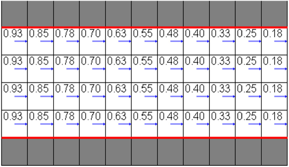
The potential field and the pedestrian desired speed direction in the corridor.

The desired speed direction in a room without obstacles

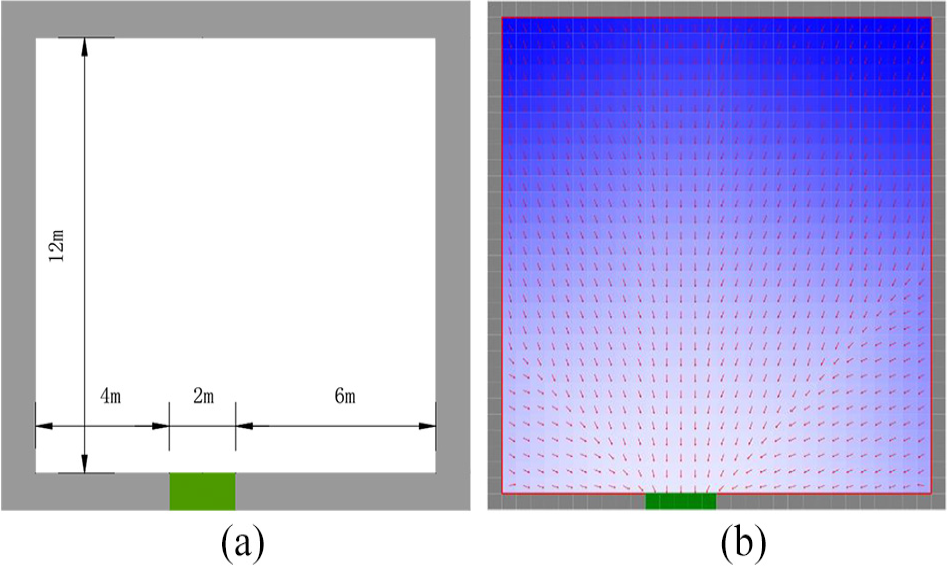
For the evacuation scene in the room without obstacles, we have a room of $12 \times 12 m^{2}$ and exit width of 2 m. The geometric parameters of the room are shown in Figure 4(a), where gray indicates the wall and green indicates the exit. Figure 4(b) demonstrates the potential field of the grid system and pedestrian desired speed direction (see the red arrows), where $μ = 0.4 m$ , $w = 1$ . In Figure 4(b), the darker the color, the larger the potential field. From Figure 4(b), we can see that the pedestrian desired speed direction ${\vec{e}}_{(x, y)}^{1}$ is along the direction of $s (x, y)$ decline, which ensures that the pedestrian moves toward the exit.

Figure 4.

The potential field and the pedestrian desired speed direction in the room without obstacles: (a) the geometric parameters of the room scene, and (b) the potential field and the pedestrian desired speed direction.

The desired speed direction around the obstacles

The motion of a pedestrian is influenced while he or she is nearby walls and obstacles. In particular, he or she always walk along borders of the walls and obstacles and try to keep a certain distance from the borders since it makes the individual uncomfortable to close the borders. This results in repulsive effects of obstacles which is considered in numerous microscopic pedestrian model, for example, the social force model described the repulsive effect as repulsive force between pedestrian and obstacles.

In our model, the repulsive effect from obstacles is also considered in the generation of the grid potential field. More specifically, we divided obstacles into grids and calculated the potential field of these grids by Step 4 of potential field algorithm in section ‘Algorithm for grid potential field’. According to the potential field of obstacle grids and equation (2), the desired speed directions of blank grids which abutting obstacle can be determined. The repulsive effect of pedestrians in the blank grids neighboring obstacles can be represented by these desired speed directions.

Figure 5 illustrated the desired speed directions of blank girds around obstacles. In Figure 5(a), the desired speed directions calculate without the potential field of obstacle grids. The desired speed directions point to the obstacle and guide pedestrian move close to the obstacle. The body of pedestrian will hit against the obstacles, and these made a mistake compared with the motion of pedestrian in fact.

Figure 5.

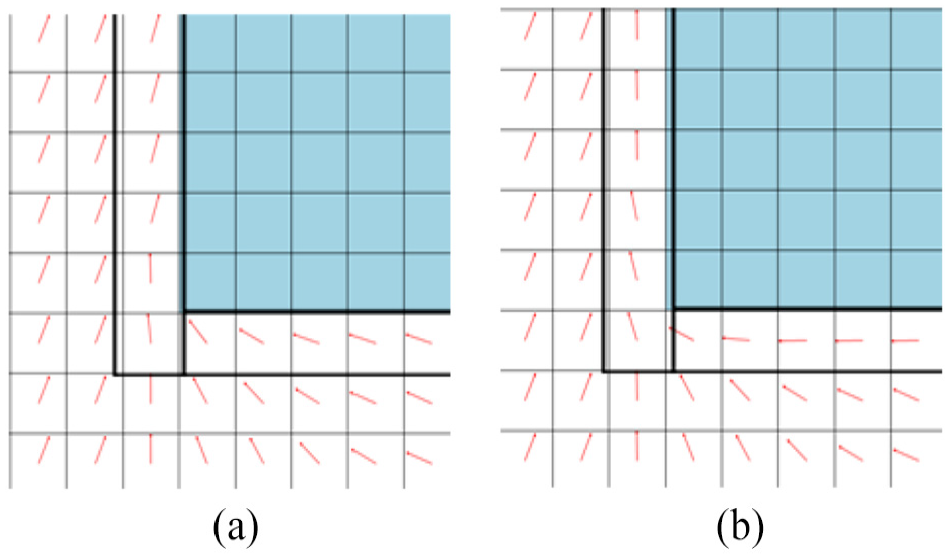
The comparison of desired direction with and without obstacle field: (a) the model without obstacle field and (b) the model with obstacle field.

Figure 5(b) displays the desired speed direction calculated with the potential field of obstacle grids. It can be seen from the figure that the arrow of desired speed directions in the blank girds abutting obstacles point along obstacles. The pedestrian in these blank grids also move along the borders of obstacles according to the desired speed directions. These indicate that the potential field of obstacle grid calculated by Step 4 in section ‘Algorithm for grid potential field’ modifies the desired speed direction in Figure 5(a), and made it a reasonable motion direction. Thus, the method can be used to simulate pedestrians’ practical movement near obstacles.

Analysis of the properties of the model

Analysis of pedestrian speed direction deviation

The tracks of pedestrian with different formulas

As described in section ‘Calculation of pedestrian speed desired direction’, the desired speed direction, which was replaced as the motion direction of pedestrian by the gradient direction at the center coordinates of the grid, is an approximate value compared with the social force model. Therefore, the difference between the approximate speed direction from our model and the accurate speed direction from the social force model would cause to a few deviations about routes of pedestrians. To examine the route deviation, we marked the trajectory of motion route of different peoples from the initial position to exit, as shown in Figure 6.

Figure 6.

Pedestrian trajectory difference in different models.

Figure 6 illustrates the route trajectory of seven individuals at different initial locations by different models. The blue line represents the trajectory record by equation (5), that is, the social force model. The green line, the yellow line, and the pink line represent the trajectory record by simulation with equations (2)–(4), respectively. It can be seen from the figure that the green line and the yellow line are basically coincident except for the trajectory line near the exit. This indicates that the potential field and equation (2) that calculate the desired speed direction formula are similar to those of the literature,³⁵ which can derive a reasonable motion path. The green line has a deviation from the blue line trajectory, and the deviation becomes more apparent as the pedestrian moves toward the exit. It is inferred that the increasing deviation has been formed by the cumulative difference between equations (2) and (5) in each grid. Compared with the deviation between the green line and the blue line, the deviation between the pink line and the blue line is more obvious, indicating that the discrepancies of the desired speed direction between equations (4) and (5) is larger than that between equations (2) and (5).

The speed direction deviation in different formulas

Figure 7 is the distribution diagram of grid cosine ${\vec{e}}_{(x, y)}^{i} (i = 1, 2, 3)$ in grid system. From Figure 7, we can see that all of the $〈 {\vec{e}}_{(x, y)}^{0}, {\vec{e}}_{(x, y)}^{i} 〉 (i = 1, 2, 3)$ are greater than $π / 4$ . It means that the three calculation methods of the pedestrian speed desired direction can guarantee that the pedestrian moves toward the exit. In general, the grid cosine distribution is basically the same in Figure 7(a) and (b), which is mostly greater than that in Figure 7(c), namely the deviation of speed direction by equation (4) from the original direction is greater than that in Guo’s model as well as our calculation method. It means that the methods based on equations (2) and (3) are better than that based on equation (4).

Figure 7.

The distribution diagram of grid cosine ${\vec{e}}_{(x, y)}^{i}$ : (a) i = 1, (b) i = 2, and (c) i = 3.

To investigate the difference between Guo’s formula and our formula in a different potential field, we give the mean and standard deviation of all the grids cosine values with the two formulas under the Guo’s potential field and our potential field, illustrated in Figure 8. As shown in Figure 8, under the same potential field, the mean and standard deviation of all the grids cosine values obtained by our formula are both smaller than that in Guo’s formula, that means the dispersion degree of grids cosine values obtained by our formula is smaller. In addition, no matter which formula is used, the mean values of all the grids cosine values in our discrete potential field are greater than that in Guo’s potential field, while the standard deviation in our discrete potential field is smaller than that in Guo’s potential field. This shows that the potential field generated in our article is slightly better than Guo’s potential field.

Figure 8.

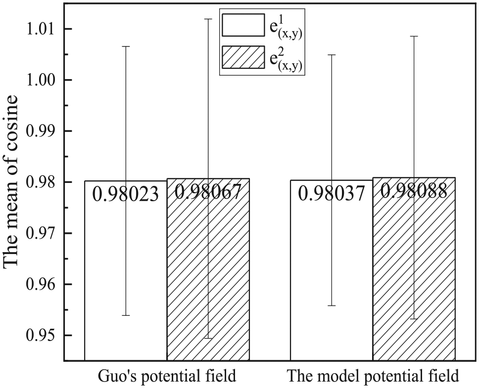
The mean and standard deviation of all grids cosine with different formulas.

By comparing our formula with Guo’s formula, we know that if there is no obstacles in the neighborhood grids $F_{(x, y)}^{m}$ of grid $(x, y)$ , we have $A = (\begin{matrix} a & 0 \\ 0 & a \end{matrix})$ , $B = P^{T}$ and the value of $a$ is related to $w$ . When $w = 1$ , we have $a = 6$ , then ${\vec{e}}_{(x, y)}^{1} = {\vec{e}}_{(x, y)}^{2}$ , which ensure $\cos 〈 {\vec{e}}_{(x, y)}^{0}, {\vec{e}}_{(x, y)}^{1} 〉 = \cos 〈 {\vec{e}}_{(x, y)}^{0}, {\vec{e}}_{(x, y)}^{2} 〉$ . These imply that the deviation of desired speed direction, which is derived from equations (2) and (3), respectively, is closely related to the grid position. To study the relationship, we divide the blank grids of simulation scene in Figure 4(a) into four types, that is, area I, area II, area III, and area IV, as shown in Figure 9. The area I consists of the grids whose distance from the surrounding wall is greater than $w$ grids. The area II consists of the grids whose distance from the wall is less than $w$ grids. The area III consists of the partial grids of area II whose distance from the wall where the exit is located is less than $w$ grids, and the area IV consists of other grids of area II except grids belong to the area III.

Figure 9.

The blank grid divided into four types of areas.

As shown in Figure 7(a) and (b), the grids cosine value distribution is the same within the area I (as shown in Figure 9), where the distance from the wall is greater than $w$ . Conversely, grids cosine value distribution is different within the areas III and IV, where the distance from the wall is smaller than $w$ . In particular, in the area of the grid near the ends of the exit, the grids cosine value in Figure 7(a) is greater than that in Figure 7(b), which proves once again that our formula is better than Guo’s formula.

During the evacuation process, pedestrian prefers to gather near the exit for a long time, so this article considers that it is more meaningful to analyze the grid cosine at the wall within the area III (see Figure 7(a)), where the exit is located. Figure 7 shows the mean and standard deviation of the cosine of grids within the area III. As shown in Figure 10, under the same potential field, the mean of these grids cosine obtained by our formula is significantly greater than that obtained by Guo’s formula within the area III, while the standard deviation of the cosine of grids is significantly smaller. This means that our formula performs better than Guo’s formula under the same potential field. Meanwhile, comparing with Guo’s potential field, under the same formula, the mean of these grids cosine in our potential field is significantly greater while the standard deviation of the cosine of grids is significantly smaller within the area III. These prove once again that our potential field is better than Guo’s potential field.

Figure 10.

The mean and standard deviation of the cosine of grids within the area III with different formulas.

Analysis of the impact of the parameters

The impact of parameters $w$

To investigate the impact of parameters $w$ on our model, the statistics of the mean of grids cosine obtained by our formula in our potential field within the area III are shown in Figure 11. As shown in Figure 11, as $w$ increases, the mean value of grids cosine within the area I gradually increases to 1.0, and the standard deviation gradually decrease, while the mean value of grids cosine within the area III gradually decreases and the standard deviation gradually increases. In general, the mean of all grids cosine value has a slight increase and then a downward trend, and the maximum appears at $w = 3$ . That is because the degree of discretization is more subtle around grid $(x, y)$ within the area I, and then ${\vec{e}}_{(x, y)}^{1}$ obtained by formula (2) is more close to the original pedestrian speed direction obtained by formula (5). Meanwhile, some wall grids around grid $(x, y)$ within the area III are not considered, and thus there are deviations between ${\vec{e}}_{(x, y)}^{1}$ and ${\vec{e}}_{(x, y)}^{0}$ . And these deviations increase as $w$ increases. When $w \leq 3$ , the grids cosine value within the area I increases more obviously than that in the areas III and IV. When $w > 3$ , the regions of the area III and IV are expanded, meanwhile, the growth of cosine of the grids in the area I is smaller than the grids in the areas III and IV. Moreover, the cosine value of all the girds in the system decreases. According to the variation of mean and standard deviation of cosine, it is better to set $w < 3$ in this model.

Figure 11.

Diagram of mean of grids cosine with $w$ in different areas.

The impact of parameters $μ$

In this subsection, we mainly investigate the impact of parameters $μ$ on our model. When μ = 0.05, 0.1, 0.2, 0.4, 0.5, 1, the statistics of the mean of grids cosine in our model are shown in Figure 12. As shown in Figure 12, the mean and standard deviation of all the grids cosine value decrease as $μ$ increases. It means that the pedestrian desired speed direction in our model gradually deviate from the original desired speed direction. It is because that the smaller the size of the grid unit, the higher the discretization precision of the scene space, which results in the smaller deviation between ${\vec{e}}_{(x, y)}^{1}$ and ${\vec{e}}_{(x, y)}^{0}$ , and the greater mean of grids cosine value. When $μ$ is small, the change of the mean value of the grids cosine is not significant, but leads to a massive calculation of the grid potential field. Therefore, $μ = 0.2 m$ is recommended in the simulation method to balance accuracy and efficiency.

Figure 12.

Diagram of mean of grids cosine values with $μ$ .

Analysis of the evacuation time

As described in section ‘Analysis of pedestrian speed direction deviation’, the pedestrian trajectory based on the model is deviated from the trajectory of the social force model. Furthermore, these deviations would lead to different evacuation times. To discuss the influence of trajectory deviation on the simulated evacuation time, we select the simulation scenario in Figure 4(a). Many repeated simulations with same pedestrian initial position distribution state are executed using the model and the social force model to calculate the simulated evacuation time of these two models. The parameters of the model are $μ = 0.2 m$ and $w = 1$ . The parameters of the social force model are $τ = 0.5$ , $A = 2000$ , $B = 0.08$ , $k_{1} = 1.2 \times 10^{5}$ , $k_{2} = 2.4 \times 10^{5}$ . Pedestrians are randomly distributed in the scene during simulation initialization. The occupancy parameter $ϕ$ denotes the pedestrian density, where $ϕ = (\sum^{N} π r_{i}^{2}) / 12 \times 12$ , $ϕ \in [0, 1]$ , and N is the total number of pedestrians. Let the evacuation time of the model be $T_{1}$ , and the evacuation time of the social force model be $T_{2}$ . We have $Δ T = T_{2} - T_{1}$ . Let $ϕ = {0, 0.002, 0.004, \dots, 0.08}$ , we repeat 50 times of the simulation for the same $ϕ$ , and count the mean and standard deviation of $Δ T$ , as shown in Figure 13.

Figure 13.

Evacuation time difference against the occupancy.

It can be seen from Figure 13 that when $ϕ$ is less than 0.038, the mean value of $Δ T$ decreases with $ϕ$ and approaches to 0. When $ϕ$ is greater than 0.038, T is approximately 0, and remains substantially unchanged with the increase of $ϕ$ . The standard deviations of the mean value of $Δ T$ also have a similar trend. This indicates that when $ϕ$ is less than 0.038, there is a difference in the evacuation time between the model and the social force model. In this case, the standard deviation of the mean value of $Δ T$ is large, indicating that the initial distribution state of pedestrians has a greater impact on $Δ T$ . This implies that when $ϕ$ is less than 0.038, the evacuation time value obtained according to the model is unreliable.

As the number of pedestrians increase, the mean and standard deviation of $Δ T$ gradually decrease. In particular, when $ϕ$ is greater than 0.038, the mean and standard deviation of $Δ T$ are both approximately 0, indicating that the simulation time of this model is close to the social force model, and the initialization of pedestrian does not affect the accuracy of the simulation time. This means that when $ϕ$ is greater than 0.038, the model is applicable to evacuation simulation. Figure 13 also shows that there is a critical occupancy $ϕ_{c}$ in the model. When $ϕ$ is greater than $ϕ_{c}$ , $Δ T$ is close to 0, and the change with $ϕ$ remains basically unchanged. Obviously, when $ϕ$ is greater than $ϕ_{c}$ , it is applicable to determine the desired direction of microscopic pedestrian simulation model based on the discrete potential field. In this model, the critical occupancy value is 0.038.

Efficiency analysis in a complex scene

As stated above, it is critical to determine the pedestrian path in the evacuation scene with obstacles. To verify the effectiveness and efficiency of our model, we have two more models as comparison,^37,38 which applies both the viewable methods to describe the spatial layout of the complex indoor evacuation scene, such as a network diagram in Figure 14(b). Based on the evacuation network, the pedestrian evacuation path is calculated by Dijkstra algorithm³⁹ and A* algorithm,⁴⁰ respectively (hereinafter referred to as Model 2 and Model 3, respectively).

Figure 14.

An evacuation scenario with one exit and obstacles: (a) evacuation scenario with obstacles and (b) the route and desire direction in the network graph.

In the literature,¹² the current position of a pedestrian was considered as O node in each simulation update step, and then find the latest shortest path to D node in the viewable network. However, we found that the pedestrian shortest path remains unchanged when the nearest node in the pedestrian distance view remains unchanged in the simulation process. Therefore, with aims to ensure the computational efficiency by Dijkstra algorithm and A* algorithm for pedestrian evacuation shortest path, we optimize the approach of determining pedestrian evacuation path as follows according to the characteristics of the network graph and the path determination process in the evacuation process. That is checking first whether the node closest to the pedestrian in the visual network changes in each simulation step: (1) if not, retain the pedestrian evacuation path or (2) otherwise, update the evacuation path according to the new OD network, where O node is the current position of the pedestrian.

To sum up, Model 1 (that is proposed in this article) mainly includes three parts: (1) calculating the discrete potential field based on the discrete space grid scene; (2) calculating the pedestrian desired speed direction according to the potential field value around the pedestrian’s grid; and (3) determining the instantaneous speed by the original direction. Meanwhile, the Models 2 and 3 consist of three parts: (1) constructing a viewable network diagram; (2) determining the moving target nodes of pedestrians in the viewable network through by A* algorithm and Dijkstra algorithm, respectively; and (3) determining the instantaneous speed by the original direction model.

The scenario in Figure 14 is set as the basic evacuation scenario, the number of obstacles in this evacuation room is $m$ , the total number of evacuation pedestrians is $n$ , and the pedestrians are randomly distributed in the evacuation room. We set m = 4, 6, 8, 10 when $n = 500$ , and n = 500, 600, 700, 800, 900, 1000 when $m = 6$ ; the social force model is adopted as the microscopic simulation model. With Microsoft Visual Studio 2010 based on dot net Framework 4.0, these experiments are operated on the platform of Window XP, CPU is Core(TM) i3-2130 2.4 GHz, 4G memory. Moreover, the same parameters are repeatedly 50 times to eliminate the distribution randomness of pedestrian in the initial state. The simulation results are shown in Tables 1 and 2.

Table 1.

Simulation time under different numbers of obstacle (unit: s).

The number of obstacles	4	6	8	10
Model 1	13.47	13.56	13.47	13.45
Model 2	34.29	50.40	94.37	168.48
Model 3	21.58	38.61	65.26	125.39

Table 2.

Simulation time under different numbers of pedestrian (unit: s).

The number of pedestrians	500	600	700	800	900	1000
Model 1	13.56	21.66	30.16	38.22	51.27	66.25
Model 2	50.40	60.36	78.88	90.17	108.65	135.69
Model 3	38.61	46.63	62.31	75.83	92.46	113.25

From Tables 1 and 2, we can see that under the same situation, the simulation time of Model 1 is significantly smaller than that of Models 2 and 3. For instance, as shown in Table 1, if there are 10 obstacles, the simulation time of Model 1 is 13.45 s, and 168.48 and 125.39 s for Models 2 and 3, respectively. Moreover, the simulation time of Model 1 is basically not affected by the change of the number of obstacles, that is, because the calculation process of the three parts of the Model 1 is basically irrelevant to the number of obstacles. But, more obstacles in the evacuation room means more nodes in the network of Models 2 and 3, that results in the following: (1) the time for constructing the viewable network in the first part of the two models increases and (2) the consumption time of the shortest path based on the network diagram in the second part also increases. Then, the total simulation time of Models 2 and 3 increases significantly. Moreover, the simulation time of Model 2 is relatively greater than that of Model 3. This is because it is more efficient to find the shortest path based on A* algorithm than Dijkstra-based algorithm in the same network.

Since, Part 2 in these models is used to determine the target node for each pedestrian, the simulation time in Part 2 increases as the number of pedestrian increases. Thus, the simulation time of the three models increases as the number of pedestrians increases, as shown in Table 2. Overall, the computational complexity of Part 2 in Model 1 is $O (n)$ , in Model 2 is $O (n^{2})$ , and Model 3 is $O (nlogn)$ . It indicates that the calculation efficiency is from high to low, that is, Model 1, Model 3, and Model 2.

Conclusion

For the pedestrian evacuation simulation model of indoor complex evacuation scenarios, it is difficult to determine the pedestrian speed expectation direction with the continuous space simulation model represented by the social force model, while their operation efficiency is relatively low. Hence, the article focuses on the characteristics of the discrete potential field to better describe the spatial layout of indoor complex scenes and establishes an improved path planning model based on the discrete potential field to determine the expected direction of pedestrian speed.

In this article, a new method of calculating the discrete potential field is put forward first, followed by the desired speed along with the gradient descent direction calculation formula. We verify first the validity of the proposed model in a corridor, then some comparative analyses with Guo’s formula and Sun’s formula are given in the indoor evacuation scene from the perspective of the cosine angle of the velocity expectation direction to verify the accuracy of our model. The results show that our formula performances are better than the both mentioned formulas. Meanwhile, the computational efficiency of our model is demonstrated in a complex evacuation scene. While, the applicable conditions and parameter range of the model are also investigated.

In general, the comparative results show that the discrete potential field idea derived from the cellular automaton model is more efficient and robust for the continuous simulation model, while it also can greatly improve the evacuation efficiency of pedestrian simulation in complex scenes.

Footnotes

Handling Editor: James Baldwin

Declaration of conflicting interests

The author(s) declared no potential conflicts of interest with respect to the research, authorship, and/or publication of this article.

Funding

The author(s) disclosed receipt of the following financial support for the research, authorship, and/or publication of this article: This work is supported by the National Key R&D Program of China (2016YFB1200402, 2019YFB1600204), Project of Beijing Talent Fund (2016000021223ZK33), Beijing Postdoctoral Research foundation (201822005), and the China Postdoctoral Science Foundation (No. 2019M650413).

ORCID iD

Minghua Li

References

Helbing

Johansson

The dynamics of crowd disasters: an empirical study. Phys Rev E 2007; 75: 46–109.

Johansson

Modeling crowd turbulence by many-particle simulations. Phys Rev E 2007; 76: 046–105.

Song

, et al. New insights into turbulent pedestrian movement pattern in crowd-quakes. J Statist Mech 2013; 2013: P02028.

Gao

, et al. Simulating the dynamic escape process in large public places. Operat Res 2014; 62: 1344–1357.

Helbing

Molnar

Social force model for pedestrian dynamics. Phys Rev E 1995; 51: 4282–4286.

Helbing

Farkas

Vicsek

Simulating dynamical features of escape panic. Nature 2000; 407: 487–490.

Helbing

Farkas

Vicsek

Freezing by heating in a driven mesoscopic system. Phys Rev Lett 2000; 84: 1240–1243.

Blue

Adler

JL.

Cellular automata microsimulation for modeling bi-directional pedestrian walkways. Transport Res Part B 2001; 35: 293–312.

Tajima

Takimoto

Nagatani

Scaling of pedestrian channel flow with a bottleneck. Phys A Stat Mech Appl 2001; 294: 257–268.

10.

Kirchner

Nishinari

Schadschneider

Friction effects and clogging in a cellular automaton model for pedestrian dynamics. Phys Rev E 2003; 67: 056122.

11.

Yue

Guan

Zhang

, et al. Study on bi-direction pedestrian flow using cellular automata simulation. Phys A Stat Mech Appl 2010; 389: 527–539.

12.

Kneidl

Hartmann

Borrmann

A hybrid multi-scale approach for simulation of pedestrian dynamics. Transport Res Part C 2013; 37: 223–237.

13.

Turner

Doxa

O’Sullivan

, et al. From isovists to visibility graphs: a methodology for the analysis of architectural space. Environ Plan B 2001; 28: 103–121.

14.

Wang

Liu

SB.

A cognitive pedestrian behavior model for exploratory navigation: visibility graph based heuristics approach. Simulat Model Pract Theory 2017; 77: 350–366.

15.

Kambara

Kibe

Nishide

, et al. Context-dependent route generation scheme using network Voronoi diagrams. In: IEEE international workshop on databases for next generation researchers (SWOD 2007), Istanbul, 15 April 2007. New York: IEEE.

16.

Nakamura

Ishii

Hiyoshi

Uni-directional pedestrian movement model based on Voronoi diagrams. In: Eighth international symposium on Voronoi diagrams in science & engineering, Qingdao, China, 28–30 June 2011. New York: IEEE Computer Society.

17.

Xiao

Gao

, et al. A pedestrian flow model considering the impact of local density: Voronoi diagram based heuristics approach. Transport Res Part C 2016; 68: 566–580.

18.

Xiao

Chraibi

, et al. Investigation of Voronoi diagram based direction choices using uni-and bi-directional trajectory data. Phys Rev E 2018; 97: 052721.

19.

Šeda

Pich

Robot motion planning using generalised Voronoi diagrams. In: Proceedings of the 8th conference on signal processing, computational geometry and artificial vision, Rhodes, 20–22 August 2008. New York: ACM.

20.

Hiyoshi

Tanioka

Hamamoto

, et al. Pedestrian movement model based on Voronoi cellular automata. Transport Res Procedia 2014; 2: 336–343.

21.

Xia

Wong

Zhang

, et al. An efficient discontinuous Galerkin method on triangular meshes for a pedestrian flow model. Int J Numer Meth Eng 2008; 76: 337–350.

22.

Boguslawski

Mahdjoubi

Zverovich

, et al. Automated construction of variable density navigable networks in a 3D indoor environment for emergency response. Automat Construct 2016; 72: 115–128.

23.

Chen

Cheng

Lin

, et al. Classification-based learning by particle swarm optimization for wall-following robot navigation. Neurocomputing 2013; 113: 27–35.

24.

Hurtado

Noy

On the number of visibility graphs of simple polygons. Amsterdam: Elsevier, 2001.

25.

Kneidl

Borrmann

Hartmann

Generation and use of sparse navigation graphs for microscopic pedestrian simulation models. Adv Eng Informat 2012; 26: 669–680.

26.

Zhou

Wang

Zhu

, et al. Tangent navigated robot path planning strategy using particle swarm optimized artificial potential field. Optik 2018; 158: 639–651.

27.

Cheng

Zhu

Sun

, et al. Path planning for autonomous underwater vehicle based on artificial potential field and velocity synthesis. In: 2015 IEEE 28th Canadian conference on electrical and computer engineering, Halifax, NS, Canada, 3–6 May 2015. New York: IEEE.

28.

Stuart

Sharifi

Christensen

, et al. Crowds involving individuals with disabilities: modeling heterogeneity using fractional order potential fields and the social force model. Phys A Stat Mech Appl 2019; 514: 244–258.

29.

Fang

Hua

, et al. An extended cost potential field cellular automata model considering behavior variation of pedestrian flow. Phys A Stat Mech Appl 2016; 462: 630–640.

30.

Guo

RY.

Potential-based dynamic pedestrian flow assignment. Transport Res Part C 2018; 91: 263–275.

31.

Jian

Wong

Zhang

, et al. Perceived cost potential field cellular automata model with an aggregated force field for pedestrian dynamics. Transport Res Part C 2014; 42: 200–210.

32.

Guo

Wang

Zheng

Lane formation in pedestrian counterflows driven by a potential field considering following and avoidance behaviours. Phys A Stat Mech Appl 2015; 432: 87–101.

33.

Leng

Wang

Xiong

Pedestrian simulations in hexagonal cell local field model. Phys A Stat Mech Appl 2015; 438: 532–543.

34.

Kretz

Bönisch

Vortisch

. Comparison of various methods for the calculation of the distance potential field. In: Pedestrian and evacuation dynamics 2008 (PED2008), Wuppertal, Germany, 27–29 February 2008. Berlin Heidelberg: Springer.

35.

Guo

Huang

HJ.

Formulation of pedestrian movement in microscopic models with continuous space representation. Transport Res Part C 2012; 24: 50–61.

36.

Sun

Shi

QX.

Algorithm of pedestrians′ path planning based on discrete potential field. Traffic Safety 2009; 23: 31–33.

37.

Asano

Iryo

Kuwahara

Microscopic pedestrian simulation model combined with a tactical model for route choice behaviour. Transport Res Part C 2010; 18: 842–855.

38.

Kretz

Hengst

Roca

, et al. Calibrating dynamic pedestrian route choice with an extended range telepresence system. In: 2011 IEEE international conference on computer vision workshops (ICCV Workshops), Barcelona, 6–13 November 2011, pp.166–172. New York: IEEE.

39.

Höcker

Berkhahn

Kneidl

, et al. Graph-based approaches for simulating pedestrian dynamics in building models. In: 8th European Conference on Product and Process Modelling (ECPPM), Cork, Ireland, 14–16 September 2010. Boca Raton: CRC Press.

40.

Dijkstra

EW.

A note on two problems in connexion with graphs. Numer Mathemat 1959; 1: 269–271.

A route navigation algorithm for pedestrian simulation based on grid potential field

Abstract

Keywords

Introduction

Algorithm and model description

Algorithm for grid potential field

Calculation of pedestrian speed desired direction

Numerical results

Analysis of desired speed direction in different scene

The desired speed direction in corridor simulation scene

The desired speed direction in a room without obstacles

The desired speed direction around the obstacles

Analysis of the properties of the model

Analysis of pedestrian speed direction deviation

The tracks of pedestrian with different formulas

The speed direction deviation in different formulas

Analysis of the impact of the parameters

The impact of parameters w

The impact of parameters μ

Analysis of the evacuation time

Efficiency analysis in a complex scene

Conclusion

Footnotes

Declaration of conflicting interests

Funding

ORCID iD

References

The impact of parameters $w$

The impact of parameters $μ$