Sage Journals: Discover world-class research

Abstract

Passenger car equivalents are used to calculate capacity and evaluate service level of urban roads. This article uses the average time headway of different car following conditions to replace the total average time headway of road vehicles, and the proportion of large vehicles to improve the headway method. This article analyzes the influence of several factors such as the proportion of large vehicles, road attributes, and traffic flow on passenger car equivalents, and obtains the following conclusions: (1) the behavior of vehicles crossing the opposite lanes has an important influence on the passenger car equivalents of the road; (2) passenger car equivalents of vertical sections at the center of central isolation belt are different from those at the start of the road; (3) the road attributes affect the passenger car equivalents; and (4) the passenger car equivalents of heavy vehicles on roads that allow two-way crossover are less than the specific value, however, the passenger car equivalents of heavy vehicles in the road segment without two-way crossing-line are greater than the specific value.

Keywords

Passenger car equivalents average time headway car following conditions urban roads mixed traffic flow

Introduction

Traffic volume plays an important role in several aspects of traffic management, such as traffic flow guidance, traffic flow emergency evacuation, and so on. Obviously, the accuracy of traffic volume determines the effectiveness of these traffic management measures. In order to express traffic volume simply and accurately, the passenger car equivalency (PCE) factor was first introduced in the Highway Capacity Manual (HCM),¹ which can transfer all non-passenger car vehicles in a mixed traffic flow to produce traffic volume using passenger car units (PCUs). Over the years, various PCE calculation methods for freeways and expressways have been developed to derive more realistic PCE factors and to obtain more accurate traffic volume.

Urban traffic problems which perplex traffic engineers can be improved through traffic flow guidance, traffic flow emergency evacuation, and other traffic management measures.

The distinctions between urban road and facilities researched in existing methods are obtained in terms of land usage, density of the entry roads, and the facilities to separate two operation directions.

The land near the expressway is mostly agricultural land and industrial land, while the land near the urban road is mostly commercial land and residential land. Thus, the amount of the passenger cars running in the freeways is less than that running in the urban road. In Singapore, the vehicle population of expressway consists of 67% passenger cars, 18% commercial vehicles, and 15% motorcycles.² In Australia, the population of urban road consists of 94.87% passenger cars, 4.40% rigid vehicles, 0.70% heavy combination vehicles, and 0.03% multi-combination vehicles.³ The difference in vehicle composition leads to the difference in mutual influence between vehicles.

Due to the differences in land usage, the number of entrances per kilometer along urban roads is more than that along the freeways. The HCM specifies about 2 ramps per km in the urban freeways and 0.125 ramps per km in the rural freeways.⁴ However, about 8–10 entrances per kilometer are settled along an urban road in a medium city. Frequency of entrances setting and the land usage determines the vehicle distribution in each lane of the roads. In Singapore, for three lane freeways, the traffic volume is 39.0, 33.2, and 23.1 veh/h/lane in the fast lane, entry lane, and slow lane, respectively. Moreover, from fast lane to slow lane, the percentage of passenger cars decreases sharply; the number of passenger cars is 86.3, 68.7, and 39.6 veh/h/lane for the fast lane, entry lane, and slow lane, respectively. On the contrary, the percentage of heavy vehicles increases sharply, and the corresponding numbers are 0.0, 1.7, and 21.6 veh/h/lane. However, the trend of the number of passenger cars and heavy vehicles in urban road from fast lane to slow lane (discussed further in section “Traffic survey”) is just opposite to that of freeway.

Central obstacles placed on the freeway to separate the two driving directions lead to traffic flows in both directions undisturbed by the other. Traffic in each lane behaves in fairly similar ways due to heavy vehicles being evenly spread across the lanes.⁵ Besides central obstacles, non-physical isolation facilities such as center double dotted line are commonly used to separate the two driving directions in urban roads. In fact, non-physical isolation facilities result in traffic flows in both directions disturbed by each other. Furthermore, center double dotted line permits vehicles from one direction to cross the line to the other direction traffic flow. Hence, non-physical isolation facilities affect the traffic flow in terms of traffic flow speed, traffic volume, traffic flow continuity, and so on.

Some researchers have reported that PCE values are affected by factors such as roadway terrain (e.g. level, rolling, or mountainous), traffic regime (congested or uncongested), and traffic level.⁶ When the road changes, its geometric characteristics, the proportion of large vehicles, the traffic environment, and so on, are also different. Consequently, the impact of the same model on other vehicles changes too, leading to various PCEs.⁷ Such traffic conditions make it difficult to adequately express traffic volume of the urban roads by presented methods. Hence, specific PCE factors should be developed to suit the applications of urban roads traffic management.

The recent research about PCEs is focused mainly on the uninterrupted flow of freeways and less on interrupted traffic flow of urban roads. More entrances and various safety facilities increase the complexity of PCE methods for urban roads. Hence, a PCE method suitable for urban roads is urgently needed. This article presents a PCE method for urban roads suitable for every traffic state based on the characteristics of lower proportion of heavy vehicles in an interrupted traffic flow and sharp decreasing trend in terms of the number of heavy vehicles and traffic volume from inner middle lane to outside lane. Then, it is analyzed whether heavy vehicles have significant effects on the traffic flow conditions having low population of heavy vehicles and whether the heavy vehicles can be neglected while deriving PCE. Moreover, the influence caused by traffic volume, headway, and the management of two directions traffic flow are also discussed in this article, in terms of the effect strength and effect direction.

The remaining part of this article is structured as follows: section “Literature review” introduces the advantages, disadvantages, and the applicable conditions of the existing PCE calculation methods. Section “Methodology” proposes a new PCE calculation method based on the headway ratio (HR) method. Section “Traffic survey” describes the methods of data collection, processing, and analysis. Section “Results and discussion” verifies the effectiveness of the proposed method and analyzes the influence of road’s attributes on PCEs. Finally, section “Conclusion” contains conclusions.

Literature review

Since the concept of PCE was first introduced in the HCM,¹ various methods have been developed under different traffic environments in terms of traffic volume, traffic states, population of heavy vehicles, and road characteristics, in order to improve the applicability of methods and to derive more realistic PCE factors. The common PCE methods include HR Method, Regression Method, Simulation Method, and Capacity Method. The applicability of these methods is elaborated as follows.

HR method

The HR method was proposed by Greenshield et al.⁸ In this method, the PCE factor is derived as the ratio of the average time headway of the selected vehicle to the average time headway of the passenger car. The HR method appropriately reflects the temporal space occupied by each vehicle in the longitudinal traffic flow. As reviewed by Kimber et al.,⁹ the HR method is appropriate for successive traffic stream where vehicles can follow each other in a lane, especially the high traffic stream. In other words, this method cannot be used for some special traffic flows that cannot form regular successive vehicles flow, such as electric traffic flow and bicycle traffic flow at the intersections.

Before using this method, an assumption and an equivalent criterion should be determined first. The assumption is that the traffic flow in the road section only consists of pure cars, and the equivalent criterion is that the total headway of the interested vehicle in a pure interested vehicle flow is equal to the total headway of the passenger car in a pure passenger car. It is worth noting that the assumption of replacing the mixed traffic flow with pure passenger cars flow ignores the impact among different vehicles. Hence, scholars have been working on overcoming the disadvantage of this idealized assumption. Partha assumed a mixed traffic flow that consisted of passenger cars and interested vehicle, and equaled the total headway of the mixed flow with the total headway of a pure passenger traffic flow.¹⁰ This assumption was closer to the actual road environment, but the percentages of passenger cars and interested vehicle in the mixed traffic flow were presented.

Regression method

Two types of multiple linear regression methods were first introduced by Branston to calculate the PCE of vehicle classes at traffic signals in urban roads: one is synchronous regression and the other is asynchronous regression.¹¹ Then, Branston and Gipps¹² presented an asynchronous regression to estimate PCE at traffic signals. Fan¹³ and Yeung and Wong¹⁴ used synchronous regression on field data for expressways to gain PCEs for different vehicle classes. In synchronous regression, the dependent variable τ is field data survey time in peak traffic flow period, and the independent variable n_i is the number of vehicles of each class recorded during the survey time. Based on the assumption that survey time contains n_i headways, regression estimates of the coefficients are obtained. In asynchronous regression, the dependent variable n_i is recorded during the survey time, the independent variable n_j (i≠j) is also recorded during the survey time, and the constant term is the product of the saturation flow β₀ in PCUs per unit time and survey time τ. Based on the same assumption as asynchronous regression, regression estimates of the coefficients are obtained.

The regression method can obtain the PCEs of each class at the same time, but it only considers the volume in the traffic flow and uses the headway regression coefficient instead of the specific headway. The regression coefficient is not equivalent to the actual headway, and there are differences in the traffic volume of each vehicle during the same investigation period. Therefore, the PCEs obtained will change with the investigation time and the data counting time period. Compared with the applicability of headway method, regression method requires traffic flow not only under successive conditions but also under saturation conditions. Sometimes, the dependent variable, independent variables, and their relationship in the regression method are presumptions, which affect the diversity of variables and make the regression method limited in some conditions.

Simulation method

Simulation method was pioneered by Linzer et al.¹⁵ to analyze the factors influencing PCEs. The simulation method can provide a large amount of data under various desired combinations of conditions by adjusting the simulation parameters. The desired conditions include pure traffic flow consisting of only passenger cars or mixed traffic flow consisting of passenger cars and some designated proportion of other vehicle classes, vehicle performance, manipulated road geometry, desired traffic volume, differential speed limits, and even truck lane restriction.^16,17

However, the greatest shortcoming of the simulation method lies in the validation of the simulation models. It is difficult to establish the validity of simulation models as it requires real-world data covering a broad spectrum of traffic and geometric conditions. As a result, the data generated by simulation models cannot be assumed to adequately represent traffic behavior in the real world.⁵

Factors affecting PCEs

According to the current PCE definition, earlier versions of the HCM considered that facility type and level of service affected the PCE of freeways.^1,18 However, the current HCM considers that traffic volume, percentage of heavy vehicles, and geometric characteristics have an influence on PCEs.^4,19 Webster made the following conclusions based on simulation data of basic freeway sections: PCE tends to increase with traffic flow, free flow speed, and grade/length of grade, and PCE tends to decrease with an increase in truck percentage and number of lanes.¹⁷ It was also recommended that a validation study of the PCE values estimated in the research should be conducted using data collected in the field. Al-Kaisy⁶ used traffic simulation and found that PCEs are affected by prevailing traffic, geometric, and control conditions. Benekohal proposed that the truck type, volume, or position of truck influences the PCE, based on analyzing the data from various traffic flow conditions by traffic simulation.²⁰

Although existing studies have analyzed the above-mentioned factors affecting PCEs, the influence trend and influence degree of factors on PCE are not given. Moreover, the validity of simulation models is quite difficult as it requires real-world data covering a broad spectrum of traffic and geometric conditions.

The data generated by simulation models cannot be assumed to adequately represent traffic behavior in the real world.⁵ Moreover, considering the limitations of regression method that traffic flow should be under saturation conditions, the HR method should derive the PCE values for roads under various traffic flow status using field data. In order to overcome the disadvantage of idealized assumption due to beforehand proposition of various vehicle classes, traffic volume and proposition of various vehicle classes are introduced to improve the HR method from the aspect of reflecting the traffic flow as realistically as possible. In addition, the extent of influence and change trend of traffic volume, percentage of heavy vehicles, and traffic design on PCE under various traffic flow states are discussed because the main conclusion of factor analysis is the type of influencing factors. The results obtained in this article can be applied to road design, capacity analysis, level-of-service determination, and traffic management and control for urban roads.

Methodology

Improvement of research assumption

The PCE factor is derived as the ratio of the average time headway of the interest car to the average time headway of the passenger car. The interest car represents the vehicles that need to calculate PCE. The method is based on the assumption that the interest car flow only includes interest cars, and the passenger car flow is only composed of passenger cars. In most instances, prevailing conditions of the urban road are not ideal and the traffic flow usually contains a mix of different vehicles, that is, buses, commercial vehicles, and passenger cars.

As reviewed by Molina,²¹ the position of a vehicle in the queue had a pronounced effect on PCE for five-axle combination trucks. In order to reflect the actual traffic conditions, Partha adjusted the assumption of the method by considering the position of interested vehicles in car following conditions and predicted proportion of vehicle classes,²² which is shown in formula 1 below

{\bar{h}}_{(c_c)} + {\bar{h}}_{(x_x)} = {\bar{h}}_{(c_x)} + {\bar{h}}_{(x_c)}

(1)

where ${\bar{h}}_{c_c}$ is the mean time headway of a car followed by a car; ${\bar{h}}_{c_x}$ is the mean time headway of a car followed by a type x vehicle, ${\bar{h}}_{x_c}$ is the mean time headway of a type x vehicle followed by a car, and ${\bar{h}}_{x_x}$ is the mean time headway of a type x vehicle followed by a type x vehicle.

For formula 1, the assumption of the method cannot be established in some cases. For instance, if the type x vehicle is greater than the passenger car, the sum of ${\bar{h}}_{c_c}$ and ${\bar{h}}_{x_x}$ is not equal but greater than the sum of ${\bar{h}}_{c_x}$ and ${\bar{h}}_{x_c}$ . Besides, in practice, traffic flow changes randomly and cannot consist of various vehicles with preset and fixed proportions.

Other factors were not considered in the existing HR method, such as traffic volume and real percentage of trucks. However, traffic volume and vehicle percentage have an important influence on PCE²⁰. Huber presented a methodology for computing PCE based on the assumption that real mixed flow rates should be equivalent to pure flow rates of cars in the same traffic service level²³

q_{b} = q_{m} \cdot P_{t} \cdot PCE + q_{m} \cdot (1 - P_{t})

(2)

where q_b is the corresponding flow rate of pure cars at a certain service level (veh/h), q_m is the corresponding flow rate of mixed vehicles at a certain service level (veh/h), p_t is the proportion of large vehicles in mixed traffic flow (%), and PCE is the passenger car equivalent for heavy vehicles.

Formula 2 considers the real proportion of vehicle classes and headway, but neglects the position of interested vehicles in car following conditions which also affect the PCE.

While the HR method takes into account the position of interested vehicles in car following conditions but defines headway and proportion of vehicle classes, Huber’s formula, by contrast, makes use of real headway and proportion of vehicle classes while neglecting the position of interested vehicles in car following conditions. This article uses the hypothesis of Huber’s formula to improve the hypothesis of the HR method for reflecting the real traffic flow.

Based on the equivalence criterion between mixed traffic flow and pure car flow under the same service level in Huber’s formula, the traffic flow and percentage of interested vehicle are introduced into HR method to reflect the actual headway.

Recent empirical evidence suggests that the PCE factors for free-flow conditions significantly underestimate the effect of heavy vehicles after the onset of congestion.¹⁶ Therefore, this study aims to develop PCE factors for heavy vehicles on urban secondary trunk roads during free flow, congested flow, and jam flow.

PCE derivation method

In this study, the traffic flow composed of passenger cars is referred to as “base case.”“Mixed traffic case” includes passenger cars and interesting cars. The improved HR method consists of six steps listed below, and derivation process is shown in Figure 1.

Figure 1.

The derivation process of improved headway ratio method.

Establishing equivalency equation by the hypothesis of the proposed method

The assumption of the earlier HR method recognized that the total headway of pure interested vehicle flow is equal to the total headway of pure basis vehicle flow. Mixed flows can be transformed into pure passenger car flows by HR method. Based on the equivalency criteria in this article, in order to satisfy practical traffic flow in the road, equation (3) can be written as below

H_{total - mix} = H_{total - basis}

(3)

where H_total-mix is the sum of the headway in a mixed traffic flow, and H_total-basis is the sum of the headway in a basis traffic flow.

Introducing traffic volume

Introducing the traffic volume, H_total-mix and H_total-basis can be deduced by equations (4) and (5)

H_{total - mix} = q_{m} {\bar{h}}_{total - mix}

(4)

H_{total - mix} = q_{b} {\bar{h}}_{bb}

(5)

where q_m is the number of the mixed flow rate (volume), ${\bar{h}}_{total - mix}$ is the average time headway of vehicle in the mixed traffic flow, q_b is the number of the basis flow rate (volume), and ${\bar{h}}_{bb}$ is the average time headway of passenger car in the basis flow.

Substituting equations (4) and (5) into equation (3), a certain number of passenger cars in the mixed-vehicle traffic flow are replaced with an equal number of the interest cars. Equation (1) can then be rewritten as equation (6)

q_{m} {\bar{h}}_{total - mix} = q_{b} {\bar{h}}_{bb}

(6)

Introducing the percentage of interested vehicles by Huber formula

In the equivalency equation (3), the left side of the equation is a mixed traffic flow. Therefore, on the right side of the equation, the mixed traffic flow should be translated into the basis traffic flow according to practical conditions.

Using Huber formula, the right side of the equation can be shown as equation (7)

q_{b} = q_{m} p_{i} PC E_{i} + q_{m} (1 - p_{i})

(7)

where p_i is percentage of interested vehicle in the mixed traffic flow; PCE_i is the PCE for interested vehicle i.

Bringing equation (7) into equation (6), equation (7) can be rewritten as equation (8)

q_{m} {\bar{h}}_{total - mix} = [q_{m} p_{i} PC E_{i} + q_{m} (1 - p_{i})] {\bar{h}}_{bb}

(8)

Solving ${\bar{h}}_{total - mix}$

The parameter solved by equation (8) is shown as equation (9)

{\bar{h}}_{total - mix} = \frac{[q_{m} p_{i} PC E_{i} + q_{m} (1 - p_{i})] {\bar{h}}_{bb}}{q_{m}}

(9)

Establishing equivalency equation for ${\bar{h}}_{total - mix}$ by the hypothesis of the proposed method

For interested vehicles and basis vehicles, there are four following conditions in the mixed traffic flow: a basis vehicle followed by a basis vehicle, a basis vehicle followed by an interested vehicle, an interested vehicle followed by a basis vehicle, and an interested vehicle followed by an interested vehicle.

The probability that the leading vehicle is an interested vehicle is p_t, and the probability that the following vehicle is a basis vehicle is (1 – p_t). Therefore, the probability of basis vehicle following interested vehicle is shown as equation (10)

p_{ib} = p_{i} (1 - p_{i})

(10)

The probabilities of interested vehicle following basis vehicle, basis vehicle following interested vehicle, and basis vehicle following basis vehicle can be obtained in the same manner.

Based on the hypothesis of the method proposed in this article, the term h_total-mix can be deduced by equation (11)

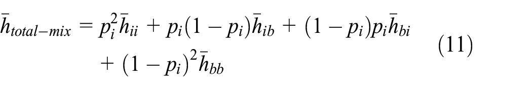
\begin{matrix} {\bar{h}}_{total - mix} = p_{i}^{2} {\bar{h}}_{ii} + p_{i} (1 - p_{i}) {\bar{h}}_{ib} + (1 - p_{i}) p_{i} {\bar{h}}_{bi} \\ + {(1 - p_{i})}^{2} {\bar{h}}_{bb} \end{matrix}

(11)

where h_tt is the average time headway for interested vehicle following interested vehicle in the mixed traffic flow, h_tb is the average time headway for interested vehicle following basis vehicle in the mixed traffic flow, h_bt is the average time headway for basis vehicle following interested vehicle in the mixed traffic flow, and h_bb is the average time headway for basis vehicle following basis vehicle in the mixed traffic flow.

Solving PCE_t

With equations (7) and (11), the relation of h_total-mix can be described as equation (12)

\begin{matrix} \frac{[q_{m} p_{i} PC E_{i} + q_{m} (1 - p_{i})] {\bar{h}}_{bb}}{q_{m}} = p_{i}^{2} {\bar{h}}_{ii} + p_{i} (1 - p_{i}) {\bar{h}}_{ib} \\ + (1 - p_{i}) p_{i} {\bar{h}}_{bi} + {(1 - p_{i})}^{2} {\bar{h}}_{bb} \end{matrix}

(12)

\begin{matrix} \frac{[q_{m} p_{t} PC E_{t} + q_{m} (1 - p_{t})] h_{b}}{q_{m}} = p 2_{t} h_{tt} + p_{t} (1 - p_{t}) h_{tb} \\ + (1 - p_{t}) p_{t} h_{bt} + (1 - p_{t}) 2 h_{bb} \end{matrix}

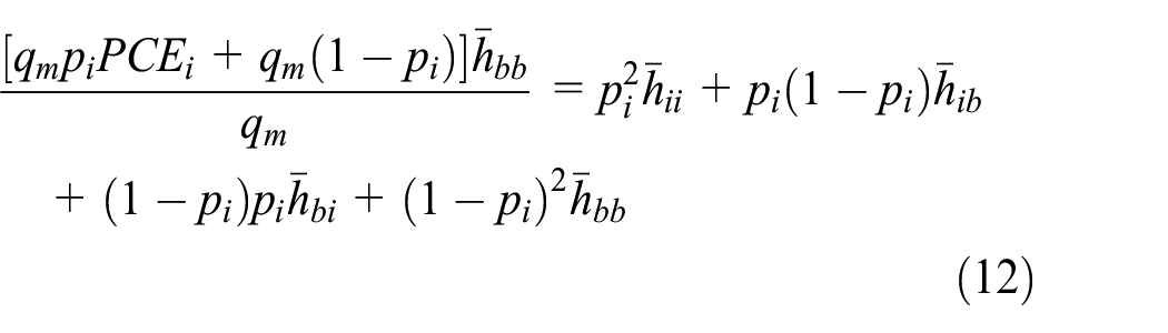
According to equation (12), the PCE_t is solved as equation (13)

PC E_{i} = \frac{p_{i} \cdot {\bar{h}}_{ii} + (1 - p_{i}) ({\bar{h}}_{ii} + {\bar{h}}_{bi} - {\bar{h}}_{bb})}{{\bar{h}}_{bb}}

(13)

Traffic survey

Sites description

In order to establish a PCE model for urban road which can be used in various traffic flow conditions and to analyze the effects of different factors on PCE values, the survey sites should be selected based on the following criteria:

The road sections should be wide, and the drivers should have a safe driving environment.

There should be no special incidents, such as road construction or traffic accident on the sections.

The geometric attributes of the survey road sections should be the same, except for the facility that divides two opposite traffic directions.

The selected roads should have similar traffic management measures, except for the measure that divides two opposite traffic directions.

Curb parking and bus stations should not be set along the selected roads.

The weather conditions should be dry without fog and haze.

The investigation period should cover a variety of traffic flow states.

The road section should be flat and straight.

The distance from upstream intersection to the survey site should be 50–200 m.^24,25

Since roads in the same area usually have similar traffic composition and management measures, the section of Hanzhongmen Street from Jiangdong North Road to Pujiang Road and the section of Qingjiang Road from Luolang Road to Mochou Road, both in JianYe district in Nanjing, Jiangsu province, China, are selected as the investigation sections as they meet the above criteria. Both the survey sites are two-lane urban secondary road segments without bus stations, having same physical separation facilities that divide non-motor vehicles and motor vehicles. The road speed limit at both these sections is 40 km/h. The characteristics of the survey road sections are shown in Table 1.

Table 1.

Attributes of the survey sections.

Site section	Number of lanes	Lane width (m)	Speed limit (km/h)	Isolation measures in bothdirections	Bus lanes
Hanzhongmen Street	4	3.75	40	Physical separation	No
Qingjiang Road	4	3.75	40	Center double dotted line	No

The difference between the two survey sections is the facility that separates two opposite motor vehicle flow directions, as shown in Figure 2. The separation facility of Hanzhongmen Street is the central green belt, a physical separation. On the contrary, Qingjiang road has center double dotted line which permits vehicles to cross the line, a non-physical separation.

Figure 2.

The plane layout of survey sections: (a) the plane layout of Hanzhongmen Street and (b) the plane layout of Qingjiang Road.

Data collection and processing

The same approach was applied to both sites, where two video cameras were used to record the motor vehicles arrival at each site. The distance from upstream intersection to the cameras should ensure that the speed at the sites should not be interrupted by intersections. In order to confirm the location of the cameras, spot speeds every fixed meters from the export of the upstream intersection to the import of the downstream intersection were surveyed by microwave radar speed guns. The initial spot of stable speed of the road section was the placement of camera 1 at both sites. Camera 2 was laid on the middle of Hanzhongmen Street and the middle of center double dotted line of Qingjiang Road. According to the criteria of selecting survey sites in section “Sites description,” the distance from upstream intersection to the survey sites should be more than 50 m. To ensure that the cameras clearly capture the road traffic condition, for Hanzhongmen Street, camera 1 was about 81 m away from the export of the upstream intersection, and the distance between two cameras was about 135 m; for Qingjiang Road, camera 1 was about 93 m away from the export of the upstream intersection, and the distance between two cameras was about 124 m. In addition, to avoid the impact of camera placement on non-motorized vehicles as much as possible, both cameras were set on the side of the non-motorized lane that close to the motorized lane. Spot speed collection at these sites was performed on 15 May 2017 from 6:30 to 8:30 a.m. The setting locations of the cameras and microwave radar speed guns on the sites are shown in Figure 2(a). The data at points 1 and 2 were recorded synchronously and during normal traffic conditions.

To determine the factors influencing PCEs under various traffic flow states, the investigation period should cover a variety of traffic flow states. In order to divide the time range of traffic flow states, the travel speeds of the sites from 6:30 to 8:30 a.m. were surveyed by two cameras. Travel speed collection at these sites took place on 16 May 2017 from 6:30 to 8:30 a.m.

Taking reference from the Road Traffic Information Service Traffic Condition Description, the traffic states of urban secondary roads can be divided into free flow, congested flow, and jam flow by two speed thresholds.²⁶ The traffic state is identified as free flow when the average speed exceeds 20 km/h and jam flow when the speed is below 10 km/h, while it is congestion flow when the speed is between these two thresholds. According to the statistics of vehicle travel speed, it is found that the average travel speeds of selected segments are 24.89, 21.89, and 20.03 km/h at 6:30–6:45 a.m., 6:45–7:00 a.m., 7:00–7:15 a.m.; 17.43 and 14.43 km/h at 7:15–7:30 a.m. and 7:30–7:45 a.m.; and 9.95, 9.81, 8.97 km/h at 7:45–8:00 a.m., 8:00–8:15 a.m., and 8:15–8:30 a.m. Thus, data were collected from 6:30 to 8:30 a.m. on 19 December 2017 and 20 December 2017, with dry motor vehicle lanes and mostly sunny weather conditions.

Characteristics of traffic volume on urban roads

In this article, the term “trucks” is used interchangeably with “heavy vehicles” to refer to the mix of heavy vehicles in the traffic stream, as the current research is concerned with all types of heavy vehicles that normally exhibit inferior performance due to higher weight-to-power ratio. Similarly, heavy vehicles are used in HCM 2016 to refer to trucks and buses.²⁷

During data processing, according to the Road Traffic Information Service Traffic Condition Description, three vehicle categories were used: passenger cars, defined as those with lengths less than 6 m and seats less than 7 m; midsize vehicles, defined as those with lengths less than 6 m and seats between 8 and 19 m, including light goods vehicles and commercial vehicles; and heavy vehicles, defined as all vehicles with lengths equal to or greater than 6 m and the seat greater than 20 m, including buses and coaches.²⁶ A total of 2341 vehicles over the period of 120 min were observed, as listed in Table 2.

Table 2.

Lane-wise traffic volume of urban roads.

			Hanzhongmen Street		Qingjiang Road
			Volume (vehicle)	%	Volume (vehicle)	%
Inside lane	Small vehicles		652	90.18	202	87.44
	Midsize vehicles	Light goods	4	0.55	5	2.16
		Commercial vehicle	5	0.69	2	0.87
	Heavy vehicles	Bus	55	7.61	19	8.23
		Coaches	7	0.97	3	1.30
Kerb lane	Small vehicles		880	95.55	405	86.91
	Midsize vehicles	Light goods	3	0.33	0	0.00
		Commercial vehicle	15	1.63	7	1.50
	Heavy vehicles	Bus	22	2.39	54	11.59
		Coaches	1	0.10	0	0.00
All lanes	Small vehicles		1532	93.19	607	87.09
	Midsize vehicles		27	1.64	14	2.00
	Heavy vehicles		85	5.17	76	10.91

Table 2 summarizes the volume of the urban roads. It can be seen that (1) the heavy vehicles on the urban road are mainly buses; (2) in Hanzhongmen Street, the proportion of small vehicles is very high, and almost always above 90%; in contrast, the proportions of heavy vehicles and midsize vehicles are very small, almost 5% and 2%. However, in Qingjiang Road, the proportion of heavy vehicles is greater, which is 10.91%; (3) the proportion of heavy vehicles on the inside lane is not uniform, and can be greater, equal, or even less than that on the curb lane due to the complex road traffic control measures. Therefore, small vehicles are chosen as the standard vehicles, and the heavy vehicles and midsize vehicles are chosen as the interest cars when calculating PCEs.

Table 2 also shows that (1) the traffic composition of heavy vehicles on freeway is mainly coaches and trucks; (2) the proportion of heavy vehicles on the freeway is greater than that on urban road, greater than 20%; and (3) the proportion of heavy vehicles on the curb lane is almost twice as much as that on the inside lane due to the lane restrictions of heavy vehicles.

In summary, the characteristics of traffic volume between urban road and freeway differ widely in terms of traffic composition, proportion of vehicle class, and distribution of traffic rate on the lane. Hence, the existing PCE method for freeway appears to be inadequate for application in urban traffic. The objective of this study is to derive PCE values for vehicles in urban traffic using headway radio method considering traffic volume and the proportion of vehicle class.

Identification of car following types

The proportion of small vehicles is 93.08% in Hanzhongmen Street, 87.09% in Qingjiang Road, and 93.06% in Hanzhong Road. The small vehicle is chosen as the standard vehicle for estimating PCE of vehicles class. The type and quantity of vehicle following conditions on urban roads are shown in Table 3.

Table 3.

The type and number of vehicle following conditions on urban roads.

Site section	Car following conditions
	pp	pm	ph	mp	mm	mh	hp	hm	hh
Hanzhongmen Street	1133	23	60	23	5	–	60	–	11
Qingjiang Road	597	11	78	12	3	–	77	–	12

pp is a small vehicle followed by a small vehicle; pm is a small vehicle followed by a medium vehicle; ph is a small vehicle followed by a heavy vehicle; mp is a medium vehicle followed by a small vehicle; mm is a medium vehicle followed by a medium vehicle; mh is a medium vehicle followed by a heavy vehicle, recorded as 23; hp is a heavy vehicle followed by a small vehicle; hm is a heavy vehicle followed by a medium vehicle; and hh is a heavy vehicle followed by a heavy vehicle.

According to the statistics of field survey data, the cases of a medium vehicle followed by a heavy vehicle (mh) and a heavy vehicle followed by a medium vehicle (hm) could not be obtained on the site sections. Therefore, mh and hm are not analyzed in this article.

In order to reflect the mutual influence of different vehicles in road sections and to improve the HR method, the average time headway of vehicles in car following condition on a mixed traffic flow was used to replace the average time headway of vehicles on a flow comprised of single vehicles type or the average time headway of vehicles on an ideal flow. Car following condition refers to the running state of vehicles in a row in a single lane.²⁸ The average time headway of vehicles under different car following conditions is the average value of the time between two successive vehicles as they pass the same point on the same lane.

Determination of data sampling intervals

Specifically, the variance of queue discharge flow (QDF) capacity observations in pcph (obtained from counts of passenger cars and heavy vehicles) during the different intervals of a data set was minimized by changing the value of the PCE factors.

The data sampling intervals to calculate the PCEs for uninterrupted traffic flow, such as expressways or highways, range from 1 to 15 min. Yeung obtained 1 min flow rates to estimate PCE for expressway locations in Singapore.⁵ Al-Kaisy et al.¹⁹ aggregated over 15 min intervals to obtain PCE for heavy vehicles on freeways located in Canada during QDF. Fan utilized traffic flow data for each 15-min interval to account for the PCE in Singapore expressways by multiple linear regression.¹³

Compared with uninterrupted traffic flow, traffic flows on urban roads are often interrupted by intersections and roadsides. It is necessary to re-evaluate the data sampling intervals. Al-Kaisy et al.¹⁹ recognized that data sampling intervals should allow sufficient observations for optimization runs and keep random fluctuation. Yeung et al.⁵ verified the stability of traffic flow using the standard deviation of the traffic stream in each lane that was less than 5. In this study, the standard deviations of the headway on car following types are used to determine the data sampling intervals for calculating PCE.

According to previous research on data sampling intervals, headways on car following types are aggregated over 1, 5, 10, 15 and 20 min intervals, respectively. Table 4 shows the standard deviations of headway for each car following types on urban road at each interval. The following analyses can be made:

The standard deviation of headway in all kinds of following types at intervals of 1 and 5 min is larger than 9 s. This result demonstrates that, for urban secondary trunk road, the traffic flow at 1-min interval and 5-min interval is unstable.

The standard deviations of headway for small vehicle and medium vehicle which are aggregated over 10 min intervals are less than 5 s. However, the standard deviation of headway for large vehicle is greater than 5 s. Therefore, 10-min interval cannot be selected to quantify PCE of the vehicle class.

The standard deviation of the average time headway for all kinds of vehicle following types at intervals of 15 and 20 min are less than 5 s, except for the condition of a heavy vehicle followed by a small vehicle, which is slightly greater than 5 s.

When the types of the two consecutive vehicles are the same, the standard deviation of average time headway decreases gradually with the increase in vehicle types. For instance, when the average time headway is counted at 15 min intervals, the standard deviation (SD) of time headway of a small vehicle followed by a small vehicle is 3.24 s, SD for a medium vehicle followed by a medium vehicle is 3.27 s, and SD for a heavy vehicle followed by a heavy vehicle is 2.35 s.

The standard deviation of the average time headway of the smaller vehicle followed by the larger vehicle is large than that of the larger vehicle followed by the smaller vehicle. For example, the standard deviation of average time headway at 15-min interval for a medium vehicle followed by a small vehicle is 3.16 s, while the standard deviation for a small vehicle followed by a medium vehicle is 3.35 s. Moreover, the standard deviation of the average time headway for a heavy vehicle followed by a small vehicle is 4.07 s, and that for a small vehicle followed by a heavy vehicle is 5.44 s.

Table 4.

Standard deviation of the average time headway at different time intervals.

Interval (min)	Standard deviation of the average time headway by car following conditions
	H₁₁(s)	H₁₂(s)	H₂₁(s)	H₂₂(s)	H₁₃(s)	H₃₁(s)	H₃₃(s)
1	9.76	9.54	9.99	9.26	10.68	12.02	9.08
5	5.45	5.30	5.53	5.02	6.57	7.76	4.87
10	3.96	3.88	4.14	3.84	5.05	6.48	3.65
15	3.24	3.16	3.35	3.13	4.07	5.44	3.02
20	2.47	2.51	2.62	2.43	3.98	4.43	2.38

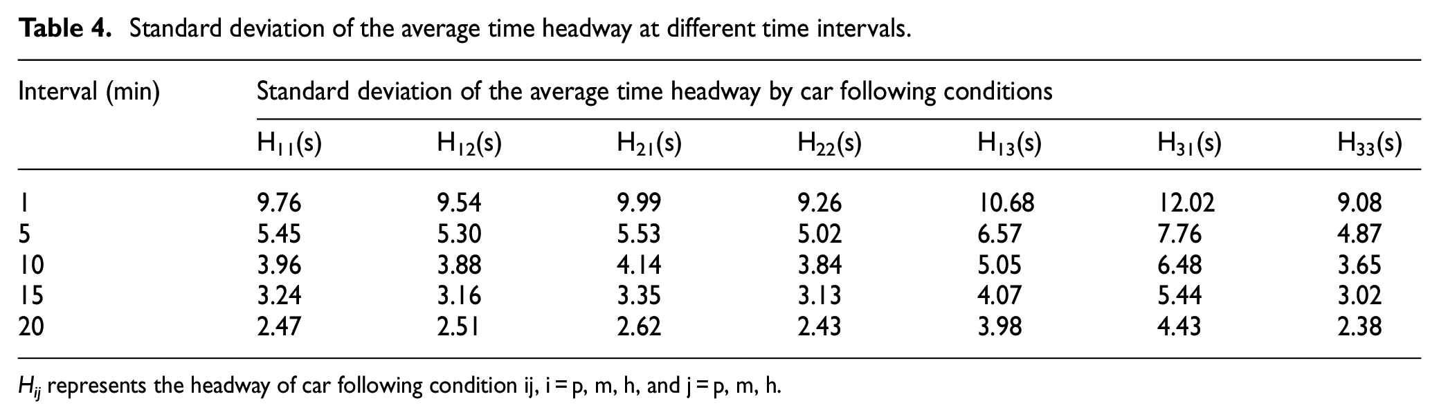
H_ij represents the headway of car following condition ij, i = p, m, h, and j = p, m, h.

From conclusions (a), (b), and (c), it can be seen that the longer the time interval, the more stable the traffic flow. Some studies suggest that with the increase of time interval, the change trend of traffic flow is less obvious and the measured data cannot reflect the changing characteristics of traffic flow.²⁹ In addition, traffic flow data are aggregated over 15 min intervals based on the fact that traffic states do not persist over longer interval.⁵ Consequently, 15-min interval is chosen herein to quantify PCE of the vehicle for urban secondary trunk roads. Conclusions (d) and (e) illustrate that there are different standard deviations of the average time headway for different car following conditions. Hence, from the perspective of traffic flow stability, it is necessary to calculate the headway by car following conditions.

Results and discussion

There are three aims to this study. One aim is to research the different effects of central isolation belt and center double dotted line on PCEs of urban secondary roads. The second aim is to analyze PCE values at different positions on the same road. The third aim is to compare the PCE values at the same positions on central isolation belt road with those on center double dotted line.

Calculation and validation

The effectiveness of the proposed method is verified by comparing with the HR method, the capacity method, and the specification in HCM. The PCE values of middle car and heavy car on Hanzhongmen Street calculated by the above three methods are shown in Table 5. It is found that

(a) The PCEs of middle cars and heavy vehicles calculated by this method are between the values of capacity method and the HR method calculated in three traffic states. For congested flow and jam flow, the PCEs calculated by proposed method are close to the values calculated by HR method. For free flow, the result is close to the value calculated by capacity method. The HR method is suitable for the traffic flow with large traffic volume. The capacity method works better for free flow. According to Leong,³⁰ the saturation flow rate based on PCE of the HR method provides better prediction than the saturation flow rate based on PCE of regression analysis.

Table 5.

PCE values calculated by different methods for different traffic flow conditions.

Traffic flow condition	Headway method		Capacity method		Specification		This article’s method		Capacity (pcu/hÿ¥
	M	H	M	H	M	H	M	H
Free	0.98	1.55	1.01	1.90	1.5	2	1.01	1.85	592
Congested	1.01	2.23	1.00	2.01	1.5	2	1.01	2.18	725
Jam	1.01	2.47	0.99	2.21	1.5	2	1.01	2.45	913

Hence, the method proposed in this study is effective for various traffic situations.

(b) Following the change in traffic flow from free flow, congestion flow to jam flow, the PCEs for heavy vehicles calculated by the proposed method show an upward trend. The maximum value appears on the jam flow and the minimum value appears on the free flow. The trend is same with the PCE value change trend calculated by the other two methods. Moreover, this result is consistent with the conclusion made by Chen.³¹ The PCE change trend from free flow to jam flow illustrates the feasibility of the proposed method.

(c) The mixed traffic flow is converted into the passenger car flow. The actual traffic volume is 555, 645, and 827 pcu/h/lane for free flow, congested flow, and jam flow, respectively. In China, the single-lane design capacity of urban secondary roads is 780 pcu/h/lane.³² The actual traffic volume is close to the designed capacity, which indicates the feasibility of the proposed method.

(d) For the middle cars, the values of PCEs calculated by the above three methods are close to 1, and similar to the PCEs of small cars. However, the specification suggests that the PCE value of middle car on the urban secondary road is 1.5. Thus, the PCE of middle car on urban secondary road vehicles suggested by the specification value is higher.

(e) For congested flow and jam flow, PCEs calculated by the three methods are larger than the specification value. The maximum PCE is 35% and the minimum is 9%. Thus, the PCEs of heavy vehicles on urban secondary roads suggested by the specification value are not appropriate.

Analysis of influence of road section attributes on PCE

The data collected from Hanzhongmen Street and Qingjiang Road are used for analysis to achieve the aims of this article. Hanzhongmen Street has central isolation belt and the car cannot cross the central isolation belt to the opposite direction lanes. Qingjiang Road has center double dotted line and the car is permitted to cross the traffic line markings to the opposite direction lanes.

The different effects of central isolation belt and center double dotted line on PCE

Analyzing the different effects of central isolation belt and center double dotted line on PCE can facilitate accurate traffic planning and determine the road design capacity. This section evaluates whether the same level roads have same PCEs and analyzes the characteristics of the PCEs trend lines on the same level roads, where only the central island facilities are not the same from free flow to jam flow.

In Figure 3, the dotted line is PCEs change trend line of Hanzhongmen Street. The dash-dot line is the PCEs change trend line of Qingjiang Road. In the period from 7:00 to 7:15 a.m., the traffic is free; from 7:30 to 7:45 a.m., the traffic flow becomes congested; and from 8:00 to 8:30 a.m., the traffic flow is jam. The following observations can be made from Figure 3:

Fitting the PCE values during the period from 7:00 to 8:30 a.m., the PCEs trend line of Hanzhongmen Street is fitted as a quadratic curve approximately and that of Qingjiang Road is fitted as a straight line approximately.

From 7:00 to 8:30 a.m., the PCEs trend line of Hanzhongmen Street is always higher than the PCEs trend line of Qingjiang Road. This indicates that, at any time, the PCEs value of Hanzhongmen Street is larger than that of Qingjiang Road.

From 7:00 to 8:30 a.m., the two trend lines increase gradually. The PCEs trend line of Hanzhongmen Street increases more than that of Qingjiang Road. The distances of the PCEs values at the same times increase as time goes on.

Figure 3.

PCEs of road sections which allow two-way traveling across the lines under different traffic conditions.

It can be deduced that the behavior of vehicles crossing the opposite lanes has an important influence on the PCEs of the road. The PCEs of the road where vehicles are not permitted to cross the opposite lanes are larger than that of the road where vehicles are permitted to cross the opposite lanes. According to the relationship between PCE and the capacity, it can be found that the capacity of the road with central isolation belt is larger than that of the road with center double dotted line. Therefore, before the road planning or design, the capacity of each road should be determined on the basis of the road central isolation facilities.

PCE values at same positions on two roads where only the central island facility is not same

The objective of this section is to discuss whether the PCEs of the same locations are the same between two roads where only the central island facility is not the same, and to analyze the influence of the central island facility on the PCEs of the road’s entrance and center.

The PCEs change trend lines at sections 1 and 2 from free flow to jam flow are shown in Figure 4. The PCEs change trend line of section 1 is fitted as dotted line, the PCEs change trend line of section 2 is fitted as dotted line, and the PCEs change trend line of the road is fitted as dash-dot line. The following observations can be made:

At the road’s entrance section, the PCEs of Hanzhongmen Street and Qingjiang Road are all fitted as binomial curves. The difference in PCE values for free flow is slight. From free flow to jam flow, the PCE values of Hanzhongmen Street rise gradually. In contrast, the PCE values of Qingjiang Road decrease gradually. Therefore, the difference in PCE values gradually expands with the increase in flow rate.

At road’s central section, the PCEs of Hanzhongmen Street and Qingjiang Road are all fitted as binomial curves. All PCEs change trend lines increase gradually. The difference is that the slope of the PCEs change trend line of Hanzhongmen Street is larger than that of the Qingjiang Road. Thus, the difference in PCEs value increases from free flow to jam flow.

In general, the difference in PCE values at the road’s entrance section is larger than that at the road’s central section.

Figure 4.

PCE values at same positions on two roads where only the central island facility is not same.

PCE values at different positions on a road

This section investigates whether the PCEs are the same at different points on a road, and evaluates which points have the greatest impact on the PCE.

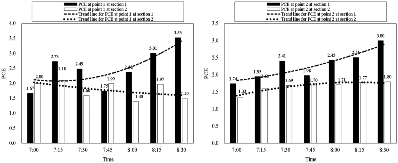
As shown in Figure 2, two vertical sections are selected from Hanzhongmen Street and Qingjiang Road, respectively. One vertical section is more than 50 m away from the intersection exit road on each road, which is marked as section 1. For Hanzhongmen Street, the other vertical section is located in the center of central isolation belt; for Qingjiang Road, the other vertical section is located in the center of center double dotted line. The other vertical section is marked section 2. The PCEs change trend lines at sections 1 and 2 from free flow to jam flow are shown in Figure 5. In Figure 5, PCEs change trend line of section 1 is fitted as dotted line, the PCEs change trend line of section 2 is fitted as dash-dot line, and the PCEs change trend line of road is fitted as dashed line. The following results are obtained:

For Hanzhongmen Street, the PCEs of vertical section 1, vertical section 2, and the road are all fitted as binomial curves. All the PCEs trend lines show an upward trend as the traffic flow changes from free to jam. The trend line of vertical section 2 shows obvious overlap in the trend line of the road from free flow to jam flow. The trend line of vertical section 1 and the trend line of the road appear to overlap only when the traffic is in congestion flow. In free flow, the difference between PCEs of vertical section 1 and vertical section 2 gradually decreases from 7:00 to 7:15 a.m. In jam flow, it gradually increases from 8:00 to 8:30 a.m.

For Qingjiang Road, the PCEs of vertical section 1, vertical section 2, and the road are all fitted as binomial curves too. The PCEs trend line at vertical section 1 gradually decreases from free flow to jam flow. However, the PCEs trend line at vertical section 2 and the road show the opposite trend of vertical section 1. The trend line of the road is close to that of vertical section 2 and above that of vertical section 2. In free flow, the difference in PCEs values between vertical section 2 and road gradually increases from 7:00 to 7:15 a.m. In jam flow, it gradually decreases from 8:00 to 8:30 a.m. In congestion flow, PCEs values of the vertical section 2 and road are approximately equal from 7:30 to 7:45 a.m.

Figure 5.

PCEs at different points of road sections over time: (a) road section 1 and (b) road section 2.

It can be deduced that, for a road, the PCEs of vertical sections in the center of central isolation belt are different from those at the start of the road. The PCEs at the start of the road are greater than those at the center of the central isolation belt. The PCEs of the road are close to those at the center of the central isolation facilities. For the road with the central isolation belt, PCEs should be calculated using the data collected from the section where the speed is stable. For the road with center double dotted line, PCEs should be calculated considering the influence of center double dotted line.

Conclusion

Based on the principle of equivalent impedance and actual measured data, this article uses the average time headway of different car following conditions and the proportion of each vehicle to improve the HR method. It also analyzes the influence of traffic flow and road sections allowing two-way crossover on PCEs, and draws the following conclusions.

There are differences between urban roads, highways, and urban highways. When dividing the statistical intervals of urban road surveys, 15 min is a reasonable time interval.

The behavior of vehicles crossing the opposite lanes has an important influence on the PCE of the road. The PCEs of the road where the vehicles are not permitted to cross the opposite lanes are larger than that of the road where the vehicles are permitted to cross the opposite lanes. According the relationship of PCE and the capacity, it can be found that the capacity of road with central isolation belt is greater than the capacity of road with center double dotted line. Therefore, before the road planning or design, the capacity of each road should be determined on the basis of the road central isolation facilities.

The PCEs of vertical sections in the central isolation belt are different from those at the start of the road. The PCEs at the start of the road are greater than those at the center of the central isolation belt. The PCEs of the road are close to those at the center of the central isolation facilities. For the road with the central isolation belt, PCEs should be calculated using the data collected from the section where the speed is stable. For the road with center double dotted line, PCEs should be calculated considering the influence of center double dotted line.

Traffic volume plays an important role in several aspects of traffic managements, such as traffic flow guidance, traffic flow emergency evacuation, and so on. The accuracy of traffic volume determines the effectiveness of these traffic management measures. Whether the method is applicable to other types of urban roads will be discussed, and a real-time PCEs calculation method based on this research will be studied in the future research.

Footnotes

Handling Editor: James Baldwin

Declaration of conflicting interests

The author(s) declared no potential conflicts of interest with respect to the research, authorship, and/or publication of this article.

Funding

The author(s) disclosed receipt of the following financial support for the research, authorship, and/or publication of this article: The authors would like to thank the Natural Science Foundation of China (grant nos 71501061, 71801080, and 51608171), Natural Science Foundation of Jiangsu province (grant no. BK20150821), and Science and Technology Plan of Hubei Provincial Transport Department (grant nos 2017-538-3-3, 2016-13-1-3).

References

Transportation Research Board. Special report 209, highway capacity manual. 3rd ed. Washington, DC: National Research Council, 1965.

Land Transport Authority. Annual vehicle statistics 2013. Singapore: Land Transport Authority, 2013.

Mohammed

Sara

Richard

Heavy vehicle management: restriction strategies. Transp Res Proc 2018; 21: 18–28.

Transportation Research Board. Highway capacity manual. 4th ed. Washington, DC: National Research Council, 2010.

Yeung

Wong

Secadiningrat

JR.

Lane-harmonised passenger car equivalents for heterogeneous expressway traffic. Transport Res A-Pol 2015; 78: 361–370.

Al-Kaisy

Passenger car equivalents for heavy vehicles at freeways and multilane highways: some critical issues. ITE J 2006; 76: 40–43.

Elefteriadou

Torbic

Webster

Development of passenger car equivalents for freeways, two-lane highways, and arterials. Transport Res Rec: J Transport Res B 1996; 1572: 51–58.

Greenshields

Shapiro

Erickson

EL.

Traffic performance at urban intersection. Technical report no. 1, Bureau of Highway Traffic, Yale University, New Haven, CT, 1947.

Kimber

Mcdonald

Hounsell

Passenger car units in saturation flows: concept, definition, derivation. Transport Res B-Meth 1985; 19: 39–61.

10.

Partha

Satish

Gangopadhaya

Lateral distribution of mixed traffic on two lane roads. J Transport Eng-ASCE 2006; 132: 597.

11.

Branston

Van Zuylen

The estimation of saturation flow, effective green time and passenger car equivalents at traffic signals by multiple linear regression. Transport Res 1978; 12: 47–53.

12.

Branston

Gipps

Some experience with a multiple linear regression method of estimating parameters of the traffic signal departure process. Transport Res 1981; 15: 445–458.

13.

Fan

HSL

. Passenger car equivalents for vehicles on Singapore expressways. Transport Res A-Pol 1990; 24: 391–396.

14.

Yeung

Wong

YD.

The effect of road tunnel environment on car following behaviour. Accid Anal Prev 2014; 70: 100–109.

15.

Linzer

Roess

McShane

Effect of trucks, buses, and recreational vehicles on freeway capacity and service volume. Transport Res Rec 1979; 699: 17–26.

16.

Al-Kaisy

Jung

Rakha

Developing passenger car equivalency factors for heavy vehicles during congestion. J Transport Eng-ASCE 2005; 131: 514–523.

17.

Webster

Elefteriadou

A simulation study of truck passenger car equivalents (PCE) on basic freeway sections. Transport Res B-Meth 1999; 33: 323–336.

18.

Transportation Research Board. Special report 209, highway capacity manual. 3rd ed. Washington, DC: National Research Council, 1985.

19.

Al-Kaisy

Hall

Reisman

ES.

Developing passenger car equivalents for heavy vehicles on freeways during queue discharge flow. Transport Res A-Pol 2002; 36: 725–742.

20.

Benekohal

Zhao

WX.

Delay-based passenger car equivalents for trucks at signalized intersections. Transport Res A-Pol 2000; 34: 437–457.

21.

Molina

CJ.

Development of passenger car equivalencies for large trucks at signalized intersections. ITE J 1987; 11: 33–37.

22.

Partha

Satish

Gangopadhaya

Speed distribution curves under mixed traffic on two lane roads. J Transport Eng-ASCE 2006; 132: 475–481.

23.

Huber

MJ.

Estimation of passenger-car equivalents of trucks in traffic stream. Transport Res Rec: J Transport Res B 1982; 869: 60–70.

24.

Luo

, et al. Traffic demand estimation for lane groups at signal-controlled intersections using travel times from video-imaging detectors. IET Intell Transp Sys 2017; 11: 222–229.

25.

Guo

Liu

, et al. Evaluating how right-turn treatments affect right-turn-on-red conflicts at signalized intersections. J Transport Saf Secur. Epub ahead of print 25 September 2018. DOI: 10.1080/19439962.2018.1490368.

26.

GB/T29107-2012. Road traffic information service-traffic condition description, 2012.

27.

Transportation Research Board. Highway capacity manual. 4th ed. Washington, DC: National Research Council, 2016.

28.

Zhang

Huang

Ren

, et al. Analysis method of distance headway in car following behavioral at steady regime. J Beijing Univ Technol 2010; 36: 119–222.

29.

GQ.

Study on characteristics of traffic parameters of urban roadways. MSc Thesis, Beijing University of Technology, Beijing, China, 2004.

30.

Leong

LV.

A study on saturation flow rates of through vehicles at signalized intersections based on Malaysian road conditions. PhD Thesis, University Sains Malaysia, Gelugor, Malaysia, 2004.

31.

Chen

Analysis on characteristics of the headway on the urban express. MSc Thesis, Jilin University, Changchun, China, 2012.

32.

CJJ37-2012. Code for design of urban road engineering, 2012.

Passenger car equivalents for urban roads using average time headway of car following conditions

Abstract

Keywords

Introduction

Literature review

HR method

Regression method

Simulation method

Factors affecting PCEs

Methodology

Improvement of research assumption

PCE derivation method

Establishing equivalency equation by the hypothesis of the proposed method

Introducing traffic volume

Introducing the percentage of interested vehicles by Huber formula

Solving h ¯ total − mix

Establishing equivalency equation for h ¯ total − mix by the hypothesis of the proposed method

Solving PCEt

Traffic survey

Sites description

Data collection and processing

Characteristics of traffic volume on urban roads

Identification of car following types

Determination of data sampling intervals

Results and discussion

Calculation and validation

Analysis of influence of road section attributes on PCE

The different effects of central isolation belt and center double dotted line on PCE

PCE values at same positions on two roads where only the central island facility is not same

PCE values at different positions on a road

Conclusion

Footnotes

Declaration of conflicting interests

Funding

References

Solving ${\bar{h}}_{total - mix}$

Establishing equivalency equation for ${\bar{h}}_{total - mix}$ by the hypothesis of the proposed method

Solving PCE_t