Numerical simulation of the non-uniform flow in a full-annulus multi-stage axial compressor with the harmonic balance method

Abstract

To improve the understanding of unsteady flow in modern advanced axial compressor, unsteady simulations on full-annulus multi-stage axial compressor are carried out with the harmonic balance method. Since the internal flow in turbomachinery is naturally periodic, the harmonic balance method can be used to reduce the computational cost. In order to verify the accuracy of the harmonic balance method, the numerical results are first compared with the experimental results. The results show that the internal flow field and the operating characteristics of the multi-stage axial compressor obtained by the harmonic balance method coincide with the experimental results with the relative error in the range of 3%. Through the analysis of the internal flow field of the axial compressor, it can be found that the airflow in the clearance of adjacent blade rows gradually changes from axisymmetric to non-axisymmetric and then returns to almost completely axisymmetric distribution before the downstream blade inlet, with only a slight non-axisymmetric distribution, which can be ignored. Moreover, the slight non-axisymmetric distribution will continue to accumulate with the development of the flow and, finally, form a distinct circumferential non-uniform flow field in latter stages, which may be the reason why the traditional single-passage numerical method will cause certain errors in multi-stage axial compressor simulations.

Introduction

The flow field in axial compressor is actually unsteady due to the blade row interaction and the flow separations. ¹ Usually a steady-state calculation method in conjunction with the multiple reference frame (MRF) method is used to conduct numerical simulations in a single-blade passage. To meet the increasing demands in accuracy of modern compressors, advanced design has increased the importance of unsteady phenomena during the design cycle. Traditionally, the time-domain method is applied to simulate unsteady flows; this method works very well for most of the simulations but is time consuming, especially for some long-term unsteady flows. Indeed, the unsteady simulation cost remains an obstacle for modern computational fluid dynamics (CFD) techniques. To improve the computational efficiency, a series of methods have been proposed by researchers over the world, and the harmonic balance method is one of the most efficient methods among them. For an unsteady time-periodic flow in axial compressors caused by the relative motion between rotor and stator, Fourier transformation is applied to transform the unsteady time-periodic flow into a coupled system of several steady-flow computations at different time stages of the period of interest. This system of steady-state equations can be solved efficiently by using traditional CFD methods and, thus, greatly reduce the computational cost.

Hall ² first proposed the harmonic balance method in 2002. The results show that the unsteady flow in a turbomachine can be accurately simulated with a small number of modes retained in the Fourier series representation of the flow, leading to a reduction of at least one order of magnitude compared to conventional nonlinear time-resolved CFD simulation methods. In the same year, He et al. ³ investigated the effects of circumferential distributions and the relative circumferential positioning of blades in multi-stage compressors using a nonlinear harmonic methodology. In recent decades, many researchers have contributed to the development of the harmonic balance method. In 2003, Nadarajah et al. ⁴ developed nonlinear frequency domain adjoint equations for the optimum shape design of unsteady flows and found that the computational efficiency is greatly increased. Thomas et al.^5–7 studied the nonlinear aerodynamic effects on flutter and limit-cycle oscillations for wings with the harmonic balance method. To model the unsteady flow in multi-stage turbomachinery with the harmonic balance method, Ekici and colleagues^8–11 carried out some extensions on the harmonic balance method. Later, Gopinath et al. ¹² performed a sliding mesh technique on the harmonic balance method to model the inter-row coupling interactions in multi-stage turbomachinery. Then, Huang and Ekici^13,14 applied the harmonic balance method on investigations of the unsteady flow in turbomachinery caused by self-excited vibrations and shape optimization of compressor cascades. Sicot and colleagues^15–17 modeled the rotor/stator interactions in turbomachinery using the harmonic balance method. More recently, a similar method is adopted by many other researchers to investigate various problems. They have demonstrated that accurate results can be obtained efficiently with the harmonic balance method.^18–21

In this article, the harmonic balance method is applied to investigate the unsteady flow field in a full-annulus multi-stage axial compressor. First, the numerical method and the model used in this work are introduced. To verify the validity of the numerical method, both the operating characteristics and the flow field parameters obtained by the harmonic balance method are compared with the experimental results at two stable working conditions. At last, a general view of the flow field in the compressor is carried out, and the development of the flow field in the clearance between the adjacent blade rows obtained at stable working condition is further analyzed.

Test introduction

The numerical simulations in this article were carried out on a two-stage axial compressor which is designed for experimental purpose. The entire compressor consists of two stages of rotor blades and stator blades, as well as an inlet guide vane and an outlet guide vane as shown in Figure 1. The radius of the casing is 264 mm at the inlet and 204.6 mm at the outlet, while the hub radius is 92.8 mm at the inlet and is 171 mm at the outlet. The design mass flow rate of the experimental axial compressor is 17.26 kg s⁻¹ and produces a total pressure ratio of 1.61 with a design rotating speed of 16,524 min⁻¹ at a standard condition. Details of the design parameters are shown in Table 1. Table 2 presents a summary of the design geometry parameters of each blade row.

Figure 1.

Two-stage high-speed axial compressor.

Table 1.

Design parameters of the test compressor.

Rotation speed	16,524 min−1
Mass flow rate	17.26 kg s−1
Efficiency	0.89
Total pressure ratio	1.61
Total temperature ratio	1.22

Table 2.

Geometry parameters of each blade row.

	IGV	R1	S1	R2	S2	OGV
Blade number	26	19	30	22	20	20
Chord length (mm)	25	39	23	35	32	46

IGV: inlet guide vane; OGV: outlet guide vane.

Mesh generation

To investigate the unsteady flow field in the flow field of the compressor, a full-annulus computational domain was considered in this investigation. As shown in Figure 2. The computational domain is extended both in upstream and downstream to minimize the influence of boundary conditions. At the inlet, the length of the intake passage is about five times of the first rotor blade chord. In downstream, the computational domain is extended equal to two blade chords. The HOH block-structured topology is used to define the blade passage of the compressor. To ensure the accuracy of the simulation with a limited grid number, the compressor domain was meshed very carefully, and a large grid scale is set in the center region of the blade channel, while the mesh scale near the wall region is relatively small. To speed up the simulation, a three-stage multi-grid method is applied in this work. For each single passage, the grid size of the rotor on the finest level is 81(x), 81(y), and 95(z) with 65 points on the blade surface along the axial direction. The grid size of the stator on the finest level is 81(x), 81(y), and 81(z) with 65 points on the blade surface along the axial direction (near the wall region, the first grid height is only 10⁻⁵ mm corresponding to about y⁺ = 1). At last, the grids are replicated around the annulus to generate a full-annulus computational domain with a grid number equals to about 1.68 × 10⁷ points in total. A general view of the used mesh in this work is shown in Figure 3.

Figure 2.

View of the computational domain.

Figure 3.

Surface mesh of the compressor.

Boundary conditions

At the inlet of the compressor, a total pressure boundary condition is applied. A mass flow rate boundary condition, which corresponds to various working conditions, is applied at the exit of the compressor. For the interface between rotor and stator, a sliding mesh technique, using a cubic spline interpolation at a constant radial position, is applied in order to allow the unsteady interactions between the rotor and stator. On the surface of blades, hub, and shroud, the no-slip and isothermal wall boundary conditions are applied. The rotation speed of the compressor is defined according to the experimental conditions.

Numerical setup

In this article, the finite volume method is used to solve the three-dimensional (3D) compressible Navier–Stokes equations. The one-eq1 Spalart–Allmaras turbulence model has been applied. A central differencing scheme with artificial dissipation according to Jameson’s switch type is used as the numerical scheme, and the discretization method in space is second-order accurate. To solve the discretized equations in time, the standard three-order explicit Runge–Kutta scheme is used. The in-house developed code SPARC is efficiently parallelized with the message passing interface (MPI).

The harmonic balance method

The 3D Navier–Stokes equations reads

$$\frac{\partial \mathit{U}}{\partial t}+\frac{\partial \mathit{F}}{\partial x}+\frac{\partial \mathit{G}}{\partial y}+\frac{\partial \mathit{H}}{\partial z}=\mathit{S}$$

Consider the flow field in axial compressors is periodic in time with a frequency $\omega$ , then the conservation variable vector $\mathit{U}(t)$ may be expressed with a Fourier series as follows

$$\mathit{U}\left(t\right)=\frac{a_0}{2}+\sum _{n=1}^N(a_n\cos \omega \mathrm{nt}+b_n\sin \omega \mathrm{nt})$$

where $a_0$ , $a_n$ , and $b_n$ are Fourier coefficient of the conservation variables.

Next, we note that the conservation variables at subtime levels may also be expressed in the same way, and we can construct the Fourier coefficients of the conservation variables by using 2N + 1 equally spaced points in time over one temporal period. The relations can be written in matrix form as

$$\tilde{\mathit{U}}=\mathit{E}{\mathit{U}}^{*}$$

where ${\mathit{U}}^{*}$ is the vector of conservation variables at 2N + 1 equally spaced point in time over one temporal period, $\tilde{\mathit{U}}$ is the matrix of the Fourier coefficients, and $\mathit{E}$ is the Fourier transformation matrix.

Conversely

$${\mathit{U}}^{*}={\mathit{E}}^{-1}\tilde{\mathit{U}}$$

where ${\mathit{E}}^{-1}$ is the corresponding inverse Fourier transformation matrix.

Note that the 2N + 1 sets of conservation variables equally spaced over one temporal period are coupled only through the time derivation term, which is approximated by the pseudo-spectral operator $\mathit{D}$ . Then, one can get the desired pseudo-spectral operator by making use of equation $\tilde{\mathit{U}}=\mathit{E}{\mathit{U}}^{*}$ to develop the pseudo-spectral operator $\mathit{D}$ , as follows

$$\frac{\partial {\mathit{U}}^{*}}{\partial \mathit{t}}=\frac{\partial {\mathit{E}}^{-1}}{\partial \mathit{t}}\tilde{\mathit{U}}=\frac{\partial {\mathit{E}}^{-1}}{\partial \mathit{t}}\mathit{E}{\mathit{U}}^{*}=\mathit{D}{\mathit{U}}^{*}$$

Finally, one can obtain the desired harmonic balance equations

$$\mathit{D}{\mathit{U}}^{*}+\frac{\partial {\mathit{F}}^{*}}{\partial x}+\frac{\partial {\mathit{G}}^{*}}{\partial y}+\frac{\partial {\mathit{H}}^{*}}{\partial z}={\mathit{S}}^{*}$$

Since the harmonic balance equation is similar in form to a conventional steady-state problem, it can be solved by introducing a pseudo-time term so that the equations can be marched to a steady-state condition using conventional CFD schemes with pseudo-time step integration

$$\frac{\partial {\mathit{U}}^{*}}{\partial \tau }+\mathit{D}{\mathit{U}}^{*}+\frac{\partial {\mathit{F}}^{*}}{\partial x}+\frac{\partial {\mathit{G}}^{*}}{\partial y}+\frac{\partial {\mathit{H}}^{*}}{\partial z}={\mathit{S}}^{*}$$

where $\tau$ is the pseudo-time step, used only to march the above equation to steady state. Note that the pseudo-time harmonic balance equations are similar in form to the original time-domain form of the Navier–Stokes equations so that existing well-developed steady CFD techniques may be used to efficiently solve the nonlinear harmonic balance equations, with a comparable number of iterations required. In addition, because only steady-state solutions are wanted, local time stepping and multi-grid acceleration techniques are used to speed up convergence. Compared with the dual time step method, the harmonic balance method is much more efficient. In this case, the harmonic balance method was implemented in our in-house code SPARC.

Result and discussion

The results of this article can be divided into two parts. First, in order to verify the validity of the numerical results, comparisons between the numerical and experimental results are carried out. After that, the full-annulus numerical results of the flow field are further analyzed in the second part.

Comparisons between the numerical and experimental results

At the beginning, the mesh independence study was carried out. In this article, three different meshes are generated with the total grid number equals to 2.62 × 10⁵, 2.09 × 10⁶, and 1.68 × 10⁷, which are marked as mesh1, mesh2, and mesh3, respectively. The operating characteristic line at 90% design speed is obtained both on these three meshes, which is shown below. As can be seen from the figure, there is a considerable difference between the results obtained from the mesh1 and mesh2. However, the difference between the results obtained from mesh2 and mesh3 is small, which means that the numerical results obtained on mesh2 are almost mesh independent. To make sure the accuracy of the simulation, the following numerical results are obtained from the mesh with the total grid number equals to 1.68 × 10⁷. For the harmonic balance method, a mode independence study is also necessary. This verification is conducted at the operating point with a mass flow rate equals to 15 kg s⁻¹. As we can see from the figure, the total pressure at the outlet obtained with three different modes is almost the same, indicating that the numerical simulation is already mode independence. Therefore, to save the computational resources while ensuring the computational accuracy, the following numerical simulation has been done with 1 mode on mesh3 (Figure 4).

Figure 4.

Mesh (left) and mode (right) independence verification.

Then, comparison between the experimental results and the numerical results is carried out. As a supplement, the numerical results obtained on a single passage by the commercial code NUMECA are also displaced here. As we can see from the figure, the operating characteristic line from the numerical results obtained by SPARC has the same shape as the experimental data but is generally slightly above the experimental data. This can be explained by the missing tip gap of the rotor blade in the simulations, and the turbulence model may also introduce some errors in the simulations. In addition, the intake shroud as well as the support plates was placed at the compressor inlet during the experiments, which may cause some undesired disturbance to the airflow entering the compressor. This may be another reason for the error between the experimental and numerical results. On the other hand, the numerical result obtained by NUMECA is located at the lower left of the experimental result. Near the stall condition, the calculated total pressure ratio is comparable to the SPARC computation results or experimental results. As the working flow increased, the working condition approaches to the choke flow boundary, the total pressure ratio calculated by NUMECA decreased rapidly, and a considerable error is visible compared to the experimental results. The most important difference between the two methods is that SPARC uses the sliding plane technique on the interface between adjacent blade rows, while NUMECA uses a mixing plane interface instead, which may be the main reason for the significant difference in the results. Therefore, we can conclude that the harmonic balance method used in this investigation is accurate enough to predict the working performance of the multi-stage axial compressor. Detailed measurements are made at a representative working condition. For this working condition, the compressor is operated at a mass flow rate of 16.09 kg s⁻¹ with a total pressure equals to 1.458 at the rotation speed of 14,870 min⁻¹. In the following, this representative working condition will be taken to analyze the experimental and numerical results of the internal flow field in the compressor (Figure 5).

Figure 5.

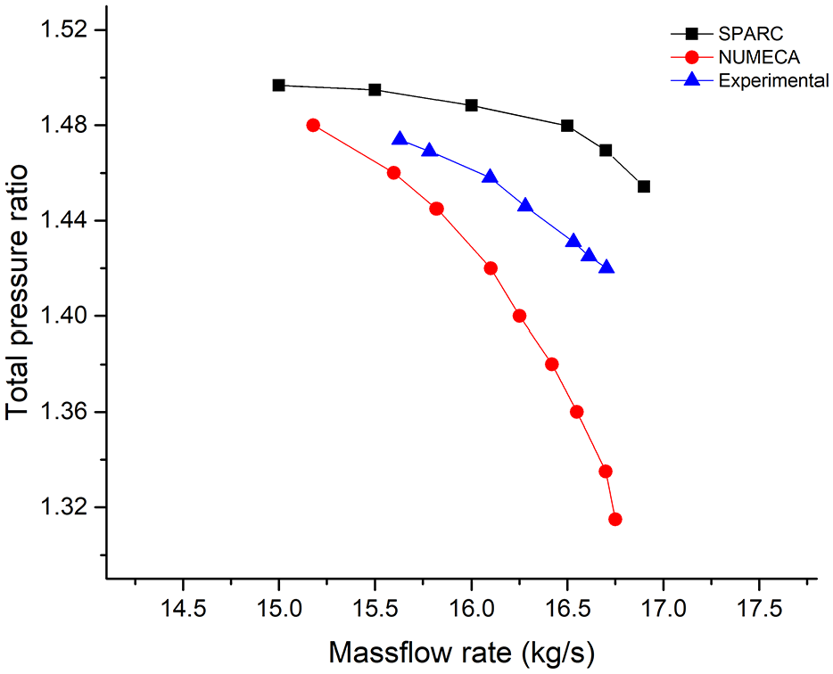
Comparison of the speed line at 90% rotating speed.

Figure 6 shows the comparison of the numerical and experimental results of the absolute velocity distribution as well as the axial flow angle distribution along the radial direction in the section just behind the first rotor blades. The experimental data used here are the mean value of thousands of data over several rotation periods measured by a 3D laser Doppler anemometry (LDA) at a certain radius, and the numerical data are the mean value of thousands of data extracted from the same radius at any instant of time. Since the internal flow field of the compressor is periodic in time at steady state, it can be considered that the average parameter on a whole ring at any instantaneous is equivalent to the experimental data measured on multiple rotation periods. It can be seen that the absolute velocity distribution in the measured section obtained by experiments and numerical simulation is essentially the same, but there is a considerable error occurred near the hub as well as the top region, with a relative maximum error in the range of 3%. In the experiments, the absolute velocity of the airflow decreases approximately linearly with the increase in the radial height; the absolute velocity obtained from the experimental data near the hub region is about 189 m s⁻¹ but is only 172 m s⁻¹ near the shroud region. After the air has passed the rotor blades, it is accelerated and a variable absolute velocity is obtained at different blade heights in order to balance the centrifugal force caused by the circumferential velocity at different blade heights. This stabilizes the flow and causes a uniform flow distribution in the compressor. Comparison of the axial flow angle distribution in the measurement plane is also given here. As before, the numerical results have the same shape as the experimental results, with a small error located at the hub and shroud region, which is in the range of 3%. The axial flow angle obtained by the experimental data is approximately 40.8° near the tip region and about 43.1° near the hub. The maximal axial flow angle is about 44.3° occurring at 25%∼45% of the blade height. It can be considered that the axial flow angle of the airflow essentially remains constant along the radial direction, which indicates that the airflow keeps stable and uniform after passing the rotor blades. In addition, as shown in the figure, the experimental results of absolute velocity and the axial flow angle are slightly smaller than the numerical results near the tip region, while near the hub region, the experimental results are slightly larger than the numerical results. As mentioned previously, the tip gap of the rotor blade is not considered in the simulations, and the gap between adjacent blade row on the hub is also not considered in the simulations, which may be the main reasons for the discrepancy presented in Figure 6. What is more, the turbulence model may also introduce some errors in the simulations, especially near the wall region.

Figure 6.

Comparison of the experimental and numerical results.

Numerical analysis of the full-annulus flow field

Similar to the last section, analysis of the flow field inside the compressor is also carried out at the representative working condition mentioned previously. Figure 7 shows the absolute velocity distribution of the flow field at 50% blade height of the compressor. It can be seen from the figure that the flow field in each passage is very similar to each other in the front blade rows so that it can be considered that the flow field is almost purely axisymmetric, while in the rear blade rows as well as in the clearance of the adjacent blade rows, the flow field in each passage is no longer purely axisymmetric, but with a slight difference between the different passages. In addition, it can also be seen that there are various degrees of high-speed flow areas on the suction side of each blade row, especially in the rear stator blades. Due to the application of the sliding plane method using an accurate cubic spline interpolation, the flow field is continuous and very smooth at the interface between rotor and stator.

Figure 7.

Absolute velocity distribution of the flow field at 50% blade height of the compressor.

Figure 8 shows the static pressure distribution of the flow field at 50% blade height of the compressor. The static pressure of the flow gradually increases along the flow direction, and there is an expected low-pressure high-speed zone at the suction side of each blade. In the passage of the two rotor blade rows, there exists a distinguishable attached oblique passage shock, which originates from the leading edge of the rotor blade and extends across the passage to 80% chord on the suction surface of the adjacent blade. This is comparable to the results at steady state by Chen et al. ²² In addition, similar to Figure 7, the static pressure distribution is basically axisymmetric in the circumferential direction in the front blade rows, but there is still some non-axisymmetric distribution in the rear blade rows as well as in the clearance between rotor and stator. In the clearance between adjacent blade rows, the flow field is affected by both the upstream and downstream blades. The wake flow generated by upstream blades continuously develops and mixes in the clearance and is additionally affected by the stagnation zone caused by the leading edge of the downstream blade. The reason for the non-axisymmetric phenomenon of the flow field in the clearance will be further analyzed in the following section.

Figure 8.

Static pressure distribution of the flow field at 50% blade height of the compressor.

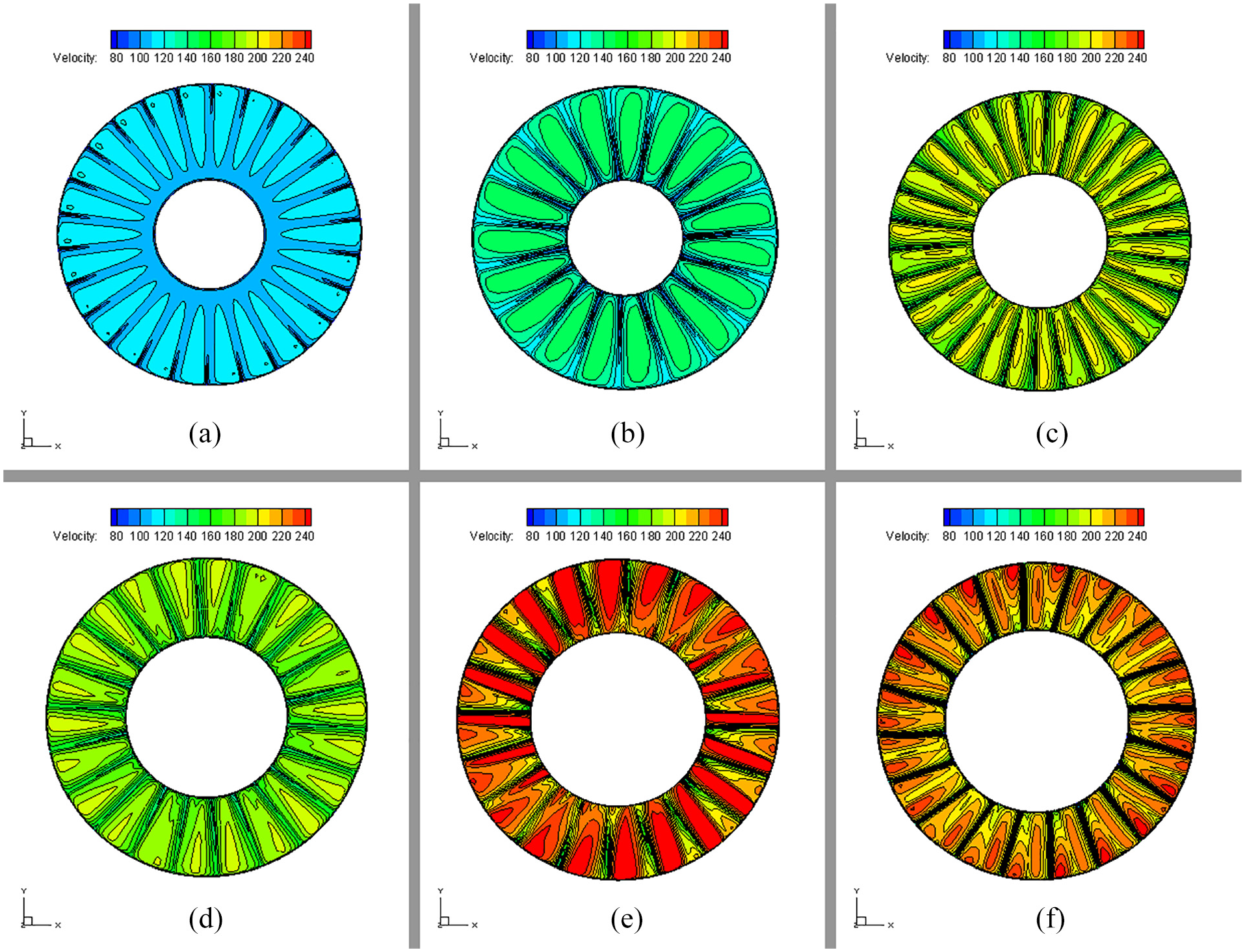
As mentioned previously, the flow field is essentially axisymmetric in the compressor, but there are some asymmetries in the clearance between rotor and stator. In this work, a sliding mesh technique is used at the interface which allows one to simulate the development process of the airflow between the rotor and stator. In order to further analyze the non-axisymmetric phenomenon and the development process of the airflow in the clearance, six axial cross-sections between the outlet of the first stage rotor and the inlet of the first stage stator are given below, which are marked as a, b, c, d, e, and f, respectively, as shown in Figure 9. Figure 9(a) is the section just after the outlet of the rotor, and section f is just before the inlet of the stator. As we can see from the figure, the flow field in Figure 9(a) is almost purely axisymmetric, and the boundary of the medium-speed zone in each passage around 75% of the blade height is almost identical. Only in the high-speed zone at the root of the blade, there exists a slight difference in the velocity distribution within each passage which can be ignored. With the air flowing downstream, the entire flow field gradually mixes and the wake flow generated by the rotor blades gradually diffuses, leading to a low-velocity zone which becomes larger and larger, as shown in Figure 9(b) and (c). Here, the flow field in the gap between adjacent blade rows is more affected by upstream blades and basically shows an axisymmetric characteristic. With the further development of the airflow, the flow field in the clearance of the rotor and stator is more affected by the downstream stator blades, resulting in corresponding changes according to the relative position of the stator blades. Since the number of stator blades and rotor blades is not equal, the relative position between the leading edge of each stator blade and each rotor blade is different, and the low-velocity zone generated at the leading edge of the stators will further interact with the wake flow produced by upstream blades, but the relative position between the low-velocity zone formed at the leading edge of each stators and the wake flow produced by the corresponding rotor blades is different, which makes the axisymmetric wake flow field produced by front blade row to be non-axisymmetric, as shown in Figure 9(d). As the flow field goes further, the different velocity zones are gradually further mixed, and the influence of downstream stator blades onto the flow field gradually increases. Then, the entire flow field gradually recovers to get axisymmetric again, but it is still non-axisymmetric at the moment shown in Figure 9(e). Before the air flows into the inlet of the downstream stator blades, the flow field is fully mixed under the effect of the downstream stator blades and turns to be an almost purely axisymmetric flow field as shown in Figure 9(f). At the end, this process will repeat in the next clearance between the rotor and stator blades. Based on the discussion above, it is clear that the flow field between rotor and stator is affected by both the wakes and potential fields, which is depending on the relative position of adjacent blade rows.

Figure 9.

Absolute velocity distribution on the cross-sections in the clearance between rotor and stator: (a) 1st section, (b) 2nd section, (c) 3rd section, (d) 4th section, (e) 5th section and (f) 6th section.

Although under the influence of the relative position of the upstream and downstream blades, the flow field in the clearance between the rotor and stator blade gradually changes from axisymmetric to non-axisymmetric and then returns back to almost purely axisymmetric before the downstream stator inlet. However, the disturbance on the entire flow field caused by the relative position of adjacent blade row is not been completely disappeared before the air flows into the downstream passage. Some detailed non-axisymmetric phenomena can still be observed at the inlet of the downstream blade. What is more important, the non-axisymmetric disturbance will not completely disappear under the rectification of the blade but will continue to accumulate with the development of the flow and, finally, form a distinct circumferential non-uniform flow field in the rear stages. Therefore, the non-axisymmetric phenomenon of the flow field at the inlet of the downstream blade is substantially negligible in former stages, while tends to be significant in later stages. Figure 10 shows the absolute velocity distribution at the inlet of each blade rows marked as a, b, c, d, e, and f, respectively. As can be seen from the figure, at the inlet of the first and second blade row, the absolute velocity distribution is both almost axisymmetric, and at the inlet of the intermediate blade row, such as the third and fourth blade row, one can see some slight non-axisymmetric distribution, but it is not very significant. In latter stages, a significant non-axisymmetric distribution can be observed. At the inlet of the fifth and sixth blade row, the flow field over the entire section is composed of four different parts; the range of the high-speed zone is smaller in the upper right and lower left side of the ring, and the range of the high-speed zone is significantly larger in the upper left and lower right side of the ring. Therefore, it can be seen that the non-axisymmetric flow caused by the difference in the relative position of each blade row still exists in the compressor even under stable conditions, and the non-axisymmetric flow continuously accumulates as the number of stage increases and, finally, leads to a considerable non-uniform flow in latter stages of the compressor. Therefore, the traditional single-passage numerical method will cause certain errors in multi-stage axial compressor simulations, and the error will increase with the increase in the number of stages. We can conclude that, in order to accurately simulate the flow field in multi-stage axial compressors, a full-annulus numerical simulation should be carried out.

Figure 10.

Absolute velocity distribution at the inlet of each blade rows: (a) inlet of row 1, (b) inlet of row 2, (c) inlet of row 3, (d) inlet of row 4, (e) inlet of row 5 and (f) inlet of row 6.

Conclusion

In this work, numerical simulation on a full-annulus multi-stage compressor is carried out with the harmonic balance method. Compared with other traditional methods, the harmonic balance method is much more efficient. To accurately model the blade row interactions, a sliding plane technique is applied at the interface between the rotor and stator, which allows the wake flow of upstream blades to further develop in downstream flow field or affect the downstream flow field through the interface between rotor and stator. In order to verify the validity of the numerical results, comparisons between the numerical results and the corresponding experimental results are first carried out. Then, the flow field in the clearance between rotor and stator in full-annulus compressor is analyzed in detail. Conclusions are summarized as follows:

First, by comparing with the experimental data, it can be said that the performance curve and flow field distribution of the compressor obtained by the numerical method are very close to the experimental results, indicating that the harmonic balance method used in this article is accurate enough to simulate the flow field of the multi-stage axial compressor.

Second, through the analysis of the internal flow field of the compressor, it can be found that the flow field is essentially axisymmetric in the compressor. However, in the clearance of the rotor and stator, there are some non-axisymmetric distributions, which may be caused by the difference in relative positions of the upstream and downstream blades in each passage. The airflow in the clearance of rotor and stator gradually changes from axisymmetric to non-axisymmetric and then returns back to almost purely axisymmetric before the downstream blade inlet.

At last, although the airflow will become axisymmetric again before entering the downstream blade, however, the disturbance on the entire flow field caused by the relative position of adjacent blade row has not been completely disappeared before the air flows into the downstream passage. Moreover, the non-axisymmetric distribution will continue to accumulate with the development of the flow and, finally, form a distinct circumferential non-uniform flow field in latter stages and may further cause rotating stall, which may be the reason that why the traditional single-passage numerical method will cause certain errors in multi-stage axial compressor simulations.