Sage Journals: Discover world-class research

Abstract

Rolling bearings are the vital components of rotary machines. The collected data of rolling bearing have strong noise interference, massive unlabeled samples, and different fault features. Thus, a deep transfer learning method is proposed for rolling bearings fault diagnosis under variable operating conditions. To obtain robust feature representation, the denoising autoencoder is used to denoise and reduce dimension of unlabeled rolling bearing signals. For those unlabeled target domain signals, a feature matching method based on multi-kernel maximum mean discrepancies between source domain and target domain is adopted to get enough labeled target domain samples. Then, these rolling bearing signals are converted to multi-dimensional graph samples and fed into a convolutional neural network model for fault diagnosis. To improve the generalization of convolutional neural network under variable operating conditions, we combine model-based transfer learning with feature-based transfer learning to initialize and optimize the convolutional neural network parameters. The effectiveness of the proposed method is validated through several comparative experiments of Case Western Reserve University data. The results demonstrate that the proposed method can learn features adaptively from noisy data and increase the accuracy rate by 2%–8% comparing with other models.

Keywords

Denoising autoencoder convolutional neural network multi-kernel maximum mean discrepancy transfer learning fault diagnosis rolling bearing

Introduction

Rolling bearings have been widely used in rotary machines. With long time and high-load operation, the rolling bearings are prone to injury and account for more than 50% of failures.¹ Thus, the fault diagnosis of rolling bearing plays a vital role in ensuring the effective operation of the mechanical system. The signals of rolling bearings include acoustic, motor current, vibration, and speed.² As vibration signals are usually easy to measure and can provide abundant dynamic information, it is commonly used in mechanical fault diagnosis.³ Traditional machine learning (ML) algorithms have been widely employed in machine fault diagnosis, including artificial neural network (ANN), support vector machine (SVM), Bayesian network, and hidden Markov model (HMM).^4–7 Nevertheless, those traditional methods require extensive domain expertise and prior knowledge, and the feature extraction is also limited in existing features or evaluation criteria. Thus, it is difficult to build a suitable model for complex fault diagnosis under variable operating conditions.⁸

As a hotspot of ML research, deep learning (DL) models can learn multiple abstract representations of big data.⁹ With the capacity of automatically extracting complex features, DL models have great potential to overcome the deficiency of traditional ML mentioned above. Several prevailing models, such as convolutional neural network (CNN), denoising autoencoder (DAE), deep belief network (DBN), and recurrent neural network (RNN), have been proposed.^10–13 These DL models have great promise in many practical applications, including image recognition, natural language processing, and machine health monitoring.^14–17 In the family of DL models, DAE is unsupervised learning algorithm based on an autoencoder (AE), while CNN is a supervised learning method. These two methods have been widely used because of their capabilities of learning complex features automatically from big data.^11,18 However, they only perform well on the abundant labeled data that are generated under the same operating conditions. To overcome the problem of lacking labeled signals and misclassification under variable operating conditions, the demand of a fault diagnosis method with great generalization ability is generated.

Transfer learning (TL) is an important means to solve the issue of collecting enough labeled data in the ML field.¹⁹ TL discovers the related features in the source task and obtains the feature mapping function $f_{s}$ in the source domain (SD). Then, it transfers $f_{s}$ to the target task and learns the feature mapping function $f_{t}$ in the SD. Therefore, the goal of TL is to improve the generalization ability of the feature mapping model by transferring the knowledge of the source domain (SD) to the target domain (TD).^20,21 Common TL methods include feature-based TL (FTL) and model-based TL (MTL). The feature-based migration can transform the features of source and target domains into the same space. Liu et al.²² implemented a domain adaptation extreme learning machine for quality prediction. Kaya et al.²³ investigated four asymmetric FTL models for plant classification. Sanodiya and Mathew²⁴ proposed a semi-supervised metric TL framework to reduce the distribution between domains both statistically and geometrically. MTL shares model parameters between source and target domains.19 Zhu et al.²⁵ proposed deep manifold regularized AEs for TL. Li et al.²⁶ developed a baseline regularization scheme for TL with CNN.

The main function of MTL is to improve the efficiency of the operation, while it is subject to limited upgrading generalization performance. FTL can use the features learned from the SD for TD analysis, but it requires a high similarity between the source and the target domains, and the distribution differences between two domains have a great influence on the classification accuracy.

Above all, a deep TL method is proposed based on CNN, DAE, and TL methods. DAE is used to reduce the sample dimension and noise interference of vibration signal. The vibration signals are transformed into multi-dimensional samples and brought into CNN for fault diagnosis. In order to improve the generalization ability of the CNN model, TL methods are used to initialize and optimize the model parameters. On the one hand, the MTL method is used to initialize the model parameters. On the other hand, through the error discrimination of the features in the source and target domains, the sample labels are initially obtained and applied for DL, so as to improve the generalization ability of FTL in the case of high distribution differences. The main contributions of this article lie in the following aspects:

The DL methods DAE and CNN are combined to process the labeled and unlabeled rolling bearing data with added noise.

The multi-kernel maximum mean discrepancy (MK-MMD) is adopted to measure the feature difference between SD and match the TD with the label of the SD.

FTL and MTL are combined to optimize the DL model for fault diagnosis of rolling bearings under various working conditions.

The rest of this article is introduced as follows: the theoretical background of DAE, CNN, TL methods is discussed in section “Theoretical background.” Section “The proposed model” presents the structure of the proposed fault diagnosis model, and related experiments are conducted to illustrate three parts of the model. Finally, the discussion and conclusion of this work are given in section “Discussion” and section “Conclusion.”

Theoretical background

In this section, we will introduce the model structure of DAE and CNN, and the definition of MK-MMD, which is usually used for feature-based migration learning.

DAE

In unsupervised learning, the most typical type of neural network is AE, which aims to get a dimensionality reduction feature $H = {h_{1}, h_{2}, h_{3}, \dots}$ from unlabeled data $X = {x_{1}, x_{2}, x_{3}, \dots}$ and take those abstract features as input to obtain the reconstructed data $\hat{X} = {{\hat{x}}_{1}, {\hat{x}}_{2}, {\hat{x}}_{3}, {\hat{x}}_{4}, {\hat{x}}_{5} \dots}$ . The network structure of an AE with a single hidden layer is shown in Figure 1. The encoder, decoder, and loss functions can be expressed as²⁷

H = σ (WX + b)

(1)

\hat{X} = σ (W' H + b')

(2)

L (X, X') = ‖ X - X' ‖^{2}

(3)

where $b$ is the bias of the input layer and $b'$ is the bias of the encoder.

Figure 1.

Structure of an autoencoder with a single hidden layer.

Traditional automatic encoders only rely on minimizing the error between input and reconstructed signal to obtain the implicit layer feature representation of input, but this training strategy may lead to over fitting and cannot guarantee the extraction of the essential features of data. The DAE with noise injection strategy enables to learn more about the essential characteristics of input data.

DAE accepts lossy data $\tilde{x}$ as input and reconstruct lossless data x by minimizing the loss function $L = - \log p_{decoder} (x | h = f (\tilde{x}))$ . The loss function in DAE is shown in Figure 2, where $C (\tilde{x} | x)$ represents the data loss process. This conditional distribution represents the probability that a given data sample x will produce a damaged sample $\tilde{x}$ . $(\tilde{x} | x)$ is used as training sample to estimate the reconstructed distribution $p_{reconstruct} (x | \tilde{x}) = p_{decoder} (x | h)$ of the DAE, where h is the output of the encoder $f (\tilde{x})$ and $p_{decoder}$ is defined according to the decoder $g (h)$ .²⁸

Figure 2.

The loss function diagram of denoising autoencoder.

CNN

CNN is one of the prevalent models for DL. Figure 3 illustrates the architecture of a typical CNN, which is a multi-stage neural network that contains many data processing layers, such as convolutional, activation, and pooling layers. The affine transformation is implemented as “Affine layer.” CNN uses convolutional layers and activation layers to extract features from the input, while the pooling layer plays a role in downsampling to make the network extract higher level features from a larger scale input. After several stacked layers of convolution and pooling, abstract features are extracted to make the classification.²⁹

Figure 3.

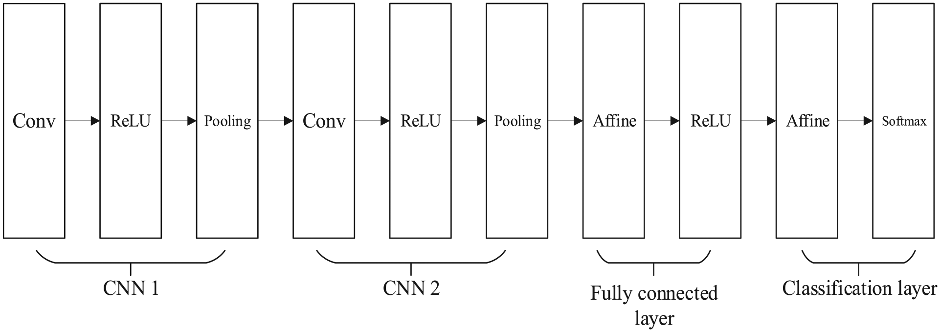
Architecture of a typical CNN.

The convolutional layers contain a number of filters, which convolute the input from the previous layer through a set of weights and compose a feature output, generally called as a feature map. The output of convolutional layers $y^{l}$ can be described as follows³⁰

y^{l} = σ (z^{l}) = σ (x^{l - 1} * W^{l} + b^{l})

(4)

σ (x) = {\begin{matrix} x & if x > 0 \\ λ x & if x \leq 0 \end{matrix}

(5)

where $x^{l - 1}$ is the input of l layer; the weight vector of l layer is the matrix $W^{l}$ ; * is a convolution operation; $b^{l}$ is the bias matrix; $z^{l}$ is the inactive output of l layer; and $σ$ is the rectified linear units (ReLU), which is used as activation function.

The main purpose of the pooling layer is to compress the image and reduce the parameters by subsampling without affecting the image quality. The pooling functions include max pooling, mean pooling, or weighted pooling. The most commonly used max pooling function in CNN can be described as³¹

p^{l} = \max_{a^{l} \in S} (y^{l})

(6)

where p is the output of the pooling layer; S is the pooling block size. The output will be S times smaller in each spatial dimension.

After multiple layers of convolution and pooling operations, the output is expanded to a fully connected layer. The softmax function is selected to achieve classification result. Assuming the classification task has K-label, the output of the softmax function can be calculated as follows³²

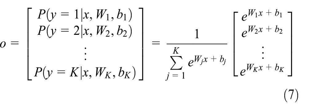
o = [\begin{matrix} P (y = 1 | x, W_{1}, b_{1}) \\ P (y = 2 | x, W_{2}, b_{2}) \\ ⋮ \\ P (y = K | x, W_{K}, b_{K}) \end{matrix}] = \frac{1}{\sum_{j = 1}^{K} e^{W_{j} x + b_{j}}} [\begin{matrix} e^{W_{1} x + b_{1}} \\ e^{W_{2} x + b_{2}} \\ ⋮ \\ e^{W_{K} x + b_{K}} \end{matrix}]

(7)

where w is the weight matrix; b is the bias matrix; and o is the output of CNN. w and b can be optimized by stochastic gradient descent (SGD) methods.³³

MK-MMD

The main challenge of TL is that there are no enough labeled samples in the TD. To resolve the problem, many researchers try to limit the deviation between the source and target domains. In this article, the MK-MMDs are applied in the proposed model to measure the error between the source and target domains.

Assume that $H_{k}$ is Hilbert space with feature kernel k . Given two probability distributions p and q for all $f \in H_{k}$ , the value of MK-MMD between p and q is defined as the reconstructed Hilbert space distance between the embedded average values of p and q. The square formula of MK-MMD can be defined as³⁴

d_{k}^{2} (p, q) \overset{Δ}{=} ‖ E_{x^{s} ~ p} [ϕ (x^{s})] - E_{x^{t} ~ q} [ϕ (x^{t})] ‖_{H_{k}}^{2}

(8)

when $ϕ$ is the feature mapping; $k (x^{s}, x^{t}) = < ϕ (x^{s}), ϕ (x^{t}) >$ is the feature kernel.

The multi-kernel k, which is defined as convex combinations of ${k_{u}}$ , can be described as³⁵

k = \sum_{u = 1}^{m} β_{u} k_{u} : \sum_{u = 1}^{m} β_{u} = 1, β_{u} \geq 0, \forall u

(9)

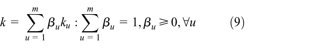
where $β_{u}$ is the weight of multi-kernel and m is the number of kernels.

The proposed model

In this article, the proposed deep TL model is the combination of DL models and TL methods. The DL models contain DAE and CNN methods, while the TL methods include feature-based and model-based TL. As shown in Figure 4, the deep TL model includes three steps as follows: data preprocessing, feature matching, and fault diagnosis. First, the DAE model is used to denoise and reduce dimension of unlabeled rolling bearing signals. Second, the MK-MMD originating from FTL is used for feature matching of the source and target domains. Third, a CNN model is built for fault diagnosis of the SD, and initial layers in CNN can be transferred for fault diagnosis of the TD. Then, the MK-MMD of the fully connected layer between the source and target domains is added in loss function to fine-tune the CNN model. Based on the above principles, a deep TL model for rolling bearing fault diagnosis under variable operating conditions is established.

Figure 4.

The structure of proposed model.

Data processing

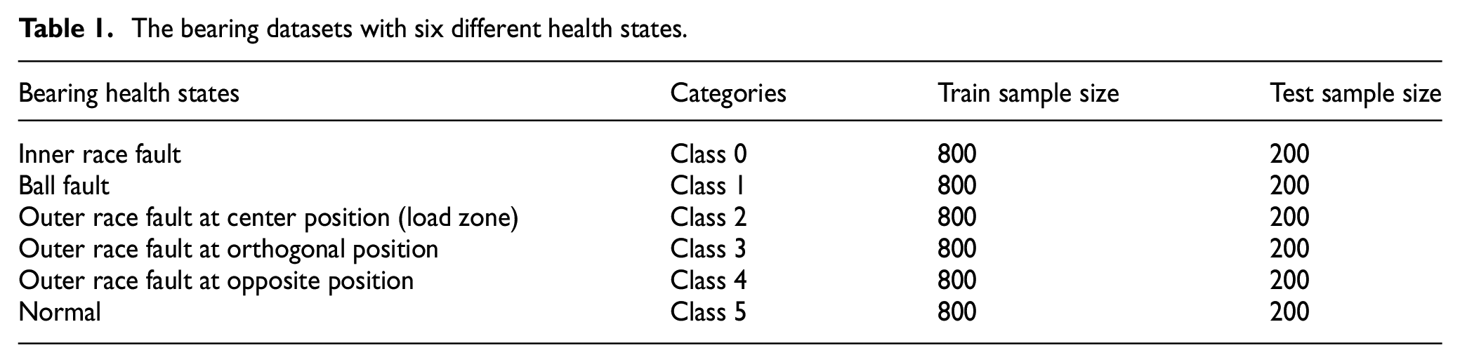
In this article, rolling bearing datasets of Case Western Reserve University are used for experiment.³⁶ Figure 5 shows the test stand of the bearing datasets. Figure 6 describes the structure of rolling bearing, which is composed of inner race, outer race, and ball. The bearing datasets with six different health states are listed in Table 1. In addition, the samples are randomly divided into training set and testing set according to the ratio of 4:1, and the cross-validation of training set is used to evaluate model performance.

Figure 5.

Test stand for rolling bearings.³⁷

Figure 6.

The structure of rolling bearing.

Table 1.

The bearing datasets with six different health states.

Bearing health states	Categories	Train sample size	Test sample size
Inner race fault	Class 0	800	200
Ball fault	Class 1	800	200
Outer race fault at center position (load zone)	Class 2	800	200
Outer race fault at orthogonal position	Class 3	800	200
Outer race fault at opposite position	Class 4	800	200
Normal	Class 5	800	200

As shown in Figure 7, the bearing datasets contain vibration signals of multiple time series. In the real industrial environments, the sensory signals are contaminated by noise. The additive Gaussian white noise (AGWN) with various standard variances Gauss noise $k σ \cdot N (0, 1)$ are added to the original vibration signals, where $k = (1, 2, 3, \dots)$ is the noise level and $σ$ is the sample variance.³⁸ Figure 8 shows the noisy signal of class 0 which made by adding original signal with Gaussian noise.

Figure 7.

Diagram of vibration signal.

Figure 8.

Noise signal with $k = 1$ .

To have enough samples for training and testing classifiers, vibration signals are split into segments with the same length of 900. Then, the added noise signals are normalized in the range [0, 1] and transformed into image sample with size 30*30.

The DAE is applied to preprocess the samples with noise. Through the training of encoder and decoder, the samples with lower dimensions can be obtained. The DAE has stacked structure of 900-600-400-600-900, which reduces the sample dimension from 30*30 to 20*20. Figure 9 shows that after 50 epochs, the mean absolute error (MAE) between the original signals and decoder gradually decreases to 0.0034, which is small enough to meet the experimental requirements.

Figure 9.

Mean absolute error of denoising autoencoder.

Feature matching based on MK-MMD

After getting the processed samples, a two-hidden-layer CNN model is built for fault diagnosis. The model parameters are listed in Table 2, where the input shape 1*20*20 means the 20*20 picture sample with 1 feature map. The SGD method and loss back propagation method are used for optimizing the model parameters.

Table 2.

Parameter setting of a CNN model with two hidden layers.

Parameter	Conv1	Conv2
Input shape	12020	41010
Input feature map	1	4
Kernel size	5	5
Stride	1	1
Padding	2	2
Maximum pooling kernel size	2	1
Output feature map	4	8
Output shape	41010	855

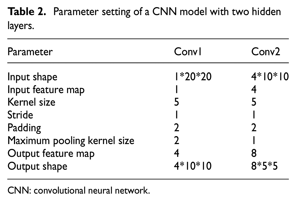
CNN: convolutional neural network.

Based on MK-MMD, a feature matching method can be used to deal with unlabeled TD. As shown in Figure 10, through calculating the MK-MMD between the unlabeled TD and SD with different categories, the category corresponding to the minimum value of MK-MMD is taken as the label of SD sample. Then, the labeled SD samples can be used for further deep TL.

Figure 10.

Feature matching based on MK-MMD.

Fault diagnosis based on deep TL

By applying TL method in DL model, the trained parameters and feature mappings in source task can be adopted to fine-tune the model of target task. In this article, the usage of TL with the CNN brings robustness to the network performance under variable operating conditions.

The structure of TL-CNN is shown in Figure 11. The original two-layer CNN can be obtained by training SD samples. Then, the parameters of the trained CNN are transferred to train TD. After convolution and polling, the MK-MMD can be calculated comparing the fully connected layers of source and target domains. Then, it can be added into the loss function of deep neural network for parameter optimization.

Figure 11.

The structure of TL-CNN.

Therefore, the optimization goal of the whole network is composed of two parts: classification error $L_{C}$ on SD and discrimination error $L_{D}$ on source and target domains. The optimizing objective L is given by Dong et al³⁹

L = L_{C} + L_{D} = min \frac{1}{n_{s}} \sum_{i = 1}^{n_{s}} J (θ (x_{i}^{s}), y_{i}^{s}) + λ \sum_{l = l_{1}}^{l_{2}} d_{k}^{2} (D_{s}^{l}, D_{t}^{l})

(10)

where $D_{s} = {(x_{i}^{s}, y_{i}^{s})}_{i = 1}^{n_{s}}$ , the $n_{s}$ annotated samples of SD. $θ (x_{i}^{s})$ is the conditional probability that the deep neural network assigns $x_{i}^{s}$ to label $y_{i}^{s}$ . $l_{1}$ and $l_{2}$ are the start and end of domain adaptive layers, respectively. $λ$ is the penalty coefficient. $J (\cdot)$ is the cross-entropy loss function. $D_{t}^{l}$ is the lth layer hidden representation of TD.

According to the value of the output layer, the final fault diagnosis results can be obtained. Figure 12 describes the training loss, which gradually decreased to 0.037 after 150 epochs. Figure 13 shows the clustering graph of fully connected layer output, which can clearly distinguish six categories and achieve 98.8% classification accuracy.

Figure 12.

The train loss of CNN.

Figure 13.

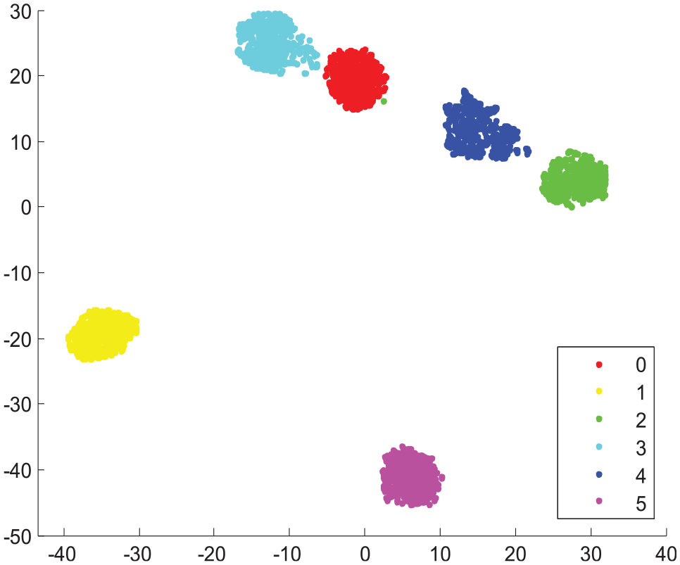
Clustering graph of fully connected layer output.

To testify the robustness of the proposed TL-CNN, different levels of noise are added into the TD samples. The cluster graphs achieved by the t-distributed stochastic neighbor embedding (t-SNE) method are shown in Figure 14.⁴⁰ With the increase in the noise level, the points in the clustering graph are more scattered, but they can still roughly distinguish the fault types and maintain high classification accuracy. It can be concluded that the proposed TL-CNN has clear cluster results and high classification accuracy under different noise levels.

Figure 14.

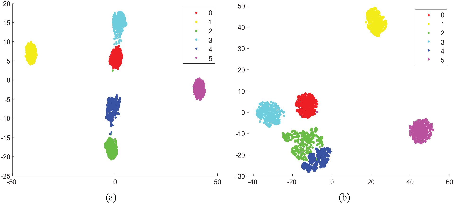
The clustering graphs of fully connected layer output with different noise. (a) Noise signal clustering graph with k = 1 (accuracy = 97.4%) and (b) noise signal clustering graph with k = 2 (accuracy = 94.1%).

Comparisons with individual DL model and traditional models

The effectiveness of the proposed TL-CNN model is validated by several comparative experiments. The SVM and ANN are classical supervised learning method, which has been widely used for fault diagnosis. DBN is the earliest DL method applied in engineering field. In addition, the CNN with model-based TL (MTL-CNN) and feature-based TL (FTL-CNN) is also selected as comparations. The parameter setting of comparison models is listed in Table 3. Besides SVM, other models have two hidden layers.

Table 3.

Parameter setting of comparison models.

Model	Node settings
TL-CNN	{400, 400, 200, 6}
MTL-CNN	{400, 400, 200, 6}
FTL-CNN	{400, 400, 200, 6}
DBN	{400, 300, 200, 6}
SVM	{400, 6}
ANN	{400, 300, 200, 6}

TL: transfer learning; CNN: convolutional neural network; MTL: model-based TL; FTL: feature-based TL; DBN: deep belief network; SVM: support vector machine; ANN: artificial neural network.

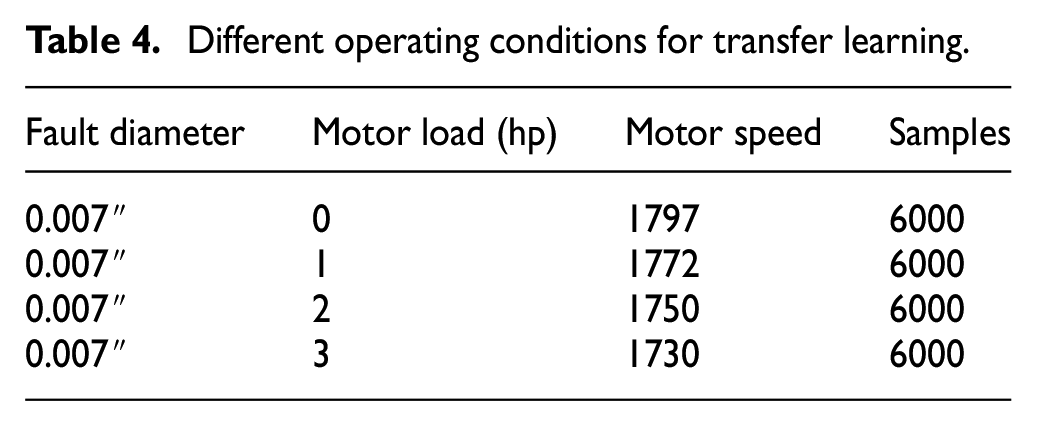
Table 4 lists different operating conditions. To testify the generalization of the proposed model, the datasets with four motor loads are selected as TD for TL.

Table 4.

Different operating conditions for transfer learning.

Fault diameter	Motor load (hp)	Motor speed	Samples
0.007″	0	1797	6000
0.007″	1	1772	6000
0.007″	2	1750	6000
0.007″	3	1730	6000

The classification accuracy with different motor loads and noise levels can be obtained in Table 5.

Table 5.

Classification accuracy (%) under different motor loads with two noise levels.

Model	SD	TD with noise 1 (k = 1)			Average	TD with noise 2 (k = 2)			Average
	Load0	Load1	Load2	Load3		Load1	Load2	Load3
TL-CNN	98.8	97.4	96.8	97.4	97.6	95.7	95.2	94.6	95.7
FTL-CNN	97.4	96.5	96.4	95.9	96.6	94.1	93	94.7	95.2
MTL-CNN	96.8	95.4	95.7	95.8	95.9	94.4	94.6	93.9	94.9
DBN	95.7	95.4	94.4	95.6	95.3	93.1	92.3	92.8	93.5
SVM	90.7	89.6	90.2	88.5	89.8	87.2	87.6	85.6	87.8
ANN	94.3	93.8	92.6	93.2	93.5	92.4	91.7	92.0	92.6

SD: source domain; TD: target domain; TL: transfer learning; CNN: convolutional neural network; FTL: feature-based TL; MTL: model-based TL; DBN: deep belief network; SVM: support vector machine; ANN: artificial neural network.

Under different operating conditions (see Figure 15), the TL-CNN has great generalization ability and can achieve higher fault diagnosis accuracy than other models. Under different noise levels (see Figure 16), the average accuracy of fault diagnosis can also be maintained at 96%, which is about 2%–8% higher than other models.

Figure 15.

Comparative experimental results under different operating conditions.

Figure 16.

Comparative experimental results under different noise levels.

Considering the engineering systems have low fault tolerance rate and big data, a little improvement of accuracy can bring huge benefits. Thus, the experimental results verify the effectiveness and feasibility of the proposed deep TL.

Discussion

Considering the noise contamination in real industrial environments, the DAE model is used to denoise and reduce dimension of unlabeled rolling bearing signals. The samples with more specific features can be obtained for further analysis. To get enough labeled TD signals, and reduce the complexity of TL for multiple fault classification, a feature match method based on MMD is adopted to compare the gap between source and target domains and choose the SD class with minimum MMD as the label of TD. To exert the powerful image processing ability of CNN, those rolling bearing signals are converted into multi-dimensional graph samples and fed into the CNN model for fault diagnosis. Based on TL, the model parameters of trained CNN with SD are transferred for training of TD. In addition, the MK-MMD of fully connected layer between source and target domains is added into loss function for optimizing the CNN model. Comparisons with individual DL model and traditional models demonstrate that the proposed TL-CNN has better generalization ability, when dealing with TD with different motor loads and fault diameters. Under different noise levels, the proposed model has great robustness, and the average accuracy of fault diagnosis can also be maintained at 96%, which is about 2%–8% higher than other models.

Conclusion

In this article, a deep TL method is proposed for rolling bearing fault diagnosis under variable operating conditions. First, DAE is used to denoise and reduce dimension of unlabeled rolling bearing signals and obtained the multi-dimensional picture samples. Second, a CNN model with several hidden layers is built for fault diagnosis of SD. Third, the trained CNN model parameters are used for the TD. In addition, the MK-MMD of fully connected layer between source and target domains is added into loss function for optimizing the CNN model. Finally, comparisons with individual DL model and traditional models demonstrate that the proposed deep TL model has better generalization ability and robustness and can maintain high fault diagnosis accuracy under variable operating conditions with noise.

Footnotes

Handling Editor: Francisco Gómez

Declaration of conflicting interests

The author(s) declared no potential conflicts of interest with respect to the research, authorship, and/or publication of this article.

Funding

The author(s) received no financial support for the research, authorship, and/or publication of this article.

ORCID iD

Changchang Che

References

Hoang

Kang

. Rolling element bearing fault diagnosis using convolutional neural network and vibration image. Cogn Syst Res 2019; 53: 42–50.

Han

Zhao

Shi

. A new fault diagnosis method based on deep belief network and support vector machine with Teager–Kaiser energy operator for bearings. Adv Mech Eng 2017; 9: 1687814017743113.

Zhu

Peng

Chen

, et al. A convolutional neural network based on a capsule network with strong generalization for bearing fault diagnosis. Neurocomputing 2019; 323: 62–75.

Wang

. Improved probabilistic neural networks with self-adaptive strategies for transformer fault diagnosis problem. Adv Mech Eng 2016; 8: 1687814015624832.

You

Shen

Guo

, et al. A hybrid technique based on convolutional neural network and support vector regression for intelligent diagnosis of rotating machinery. Adv Mech Eng 2017; 9: 1687814017704146.

Rabiei

Droguett

Modarres

. A prognostics approach based on the evolution of damage precursors using dynamic Bayesian networks. Adv Mech Eng 2016; 8: 1687814016666747.

Kamlu

Laxmi

. Condition-based maintenance strategy for vehicles using hidden Markov models. Adv Mech Eng 2019; 11: 1687814018806380.

Qiu

Cai

. A deep convolutional neural networks model for intelligent fault diagnosis of a gearbox under different operational conditions. Measurement 2019; 145: 94–107.

Han

Tang

Deng

. An enhanced convolutional neural network with enlarged receptive fields for fault diagnosis of planetary gearboxes. Comput Ind 2019; 107: 50–58.

10.

Jiao

Zhao

Lin

, et al. A multivariate encoder information based convolutional neural network for intelligent fault diagnosis of planetary gearboxes. Knowl-Based Syst 2018; 160: 237–250.

11.

Wang

Qin

, et al. Fault diagnosis of rotary machinery components using a stacked denoising autoencoder-based health state identification. Signal Process 2017; 130: 377–388.

12.

Shao

Jiang

Zhang

, et al. Rolling bearing fault feature learning using improved convolutional deep belief network with compressed sensing. Mech Syst Signal Pr 2018; 100: 743–765.

13.

Guo

Jia

, et al. A recurrent neural network based health indicator for remaining useful life prediction of bearings. Neurocomputing 2017; 240: 98–109.

14.

Zhao

. Spectral–spatial feature extraction for hyperspectral image classification: a dimension reduction and deep learning approach. IEEE T Geosci Remote 2016; 54: 4544–4554.

15.

Young

Hazarika

Poria

, et al. Recent trends in deep learning based natural language processing. IEEE Comput Intell M 2018; 13: 55–75.

16.

Zhao

Yan

Chen

, et al. Deep learning and its applications to machine health monitoring. Mech Syst Signal Pr 2019; 115: 213–237.

17.

Khan

Yairi

. A review on the application of deep learning in system health management. Mech Syst Signal Pr 2018; 107: 241–265.

18.

Janssens

Slavkovikj

Vervisch

, et al. Convolutional neural network based fault detection for rotating machinery. J Sound Vib 2016; 377: 331–345.

19.

Shin

Roth

Gao

, et al. Deep convolutional neural networks for computer-aided detection: CNN architectures, dataset characteristics and transfer learning. IEEE T Med Imaging 2016; 35: 1285–1298.

20.

Hasan

Islam

Kim

. Acoustic spectral imaging and transfer learning for reliable bearing fault diagnosis under variable speed conditions. Measurement 2019; 138: 620–631.

21.

Zhang

Zhou

. Transfer learning for short-term wind speed prediction with deep neural networks. Renew Energ 2016; 85: 83–95.

22.

Liu

Yang

Liu

, et al. Domain adaptation transfer learning soft sensor for product quality prediction. Chemometr Intell Lab 2019; 192: 103813.

23.

Kaya

Keceli

Catal

, et al. Analysis of transfer learning for deep neural network based plant classification models. Comput Electron Agr 2019; 158: 20–29.

24.

Sanodiya

Mathew

. A framework for semi-supervised metric transfer learning on manifolds. Knowl-Based Syst 2019; 176: 1–14.

25.

Zhu

, et al. Transfer learning with deep manifold regularized auto-encoders. Neurocomputing 2019; 369: 145–154.

26.

Grandvalet

Davoine

. A baseline regularization scheme for transfer learning with convolutional neural networks. Pattern Recogn 2019; 98: 107049.

27.

Struzik

Zhang

, et al. Feature learning from incomplete EEG with denoising autoencoder. Neurocomputing 2015; 165: 23–31.

28.

Xia

Liu

, et al. Intelligent fault diagnosis approach with unsupervised feature learning by stacked denoising autoencoder. IET Sci Meas Technol 2017; 11: 687–695.

29.

Fuan

Hongkai

Haidong

, et al. An adaptive deep convolutional neural network for rolling bearing fault diagnosis. Meas Sci Technol 2017; 28: 095005.

30.

Jing

Zhao

, et al. A convolutional neural network based feature learning and fault diagnosis method for the condition monitoring of gearbox. Measurement 2017; 111: 1–10.

31.

Zhang

Ding

. Cross-domain fault diagnosis of rolling element bearings using deep generative neural networks. IEEE T Ind Electron 2018; 66: 5525–5534.

32.

Jia

Lei

, et al. Deep normalized convolutional neural network for imbalanced fault classification of machinery and its understanding via visualization. Mech Syst Signal Pr 2018; 110: 349–367.

33.

Xia

, et al. Fault diagnosis for rotating machinery using multiple sensors and convolutional neural networks. IEEE/ASME T Mech 2017; 23: 101–110.

34.

Long

Zhu

Wang

, et al. Deep transfer learning with joint adaptation networks. In: Proceedings of the 34th international conference on machine learning, Sydney, NSW, Australia, 6–11 August 2017, paper no. 70, pp.2208–2217. New York: ACM.

35.

Gretton

Borgwardt

Rasch

, et al. A kernel two-sample test. J Mach Learn Res 2012; 13: 723–773.

36.

Smith

Randall

. Rolling element bearing diagnostics using the Case Western Reserve University data: a benchmark study. Mech Syst Signal Pr 2015; 64: 100–131.

37.

Boudiaf

Moussaoui

Dahane

, et al. A comparative study of various methods of bearing faults diagnosis using the Case Western Reserve university data. J Fail Anal Prev 2016; 16: 271–284.

38.

Zhang

, et al. Stochastic resonance in an asymmetric bistable system driven by multiplicative and additive Gaussian noise and its application in bearing fault detection. Chinese J Phys 2018; 56: 1173–1186.

39.

Dong

Zhang

Shi

, et al. Image deblurring and super-resolution by adaptive sparse domain selection and adaptive regularization. IEEE T Image Process 2011; 20: 1838–1857.

40.

Zheng

Jiang

Pan

. Sigmoid-based refined composite multiscale fuzzy entropy and t-SNE based fault diagnosis approach for rolling bearing. Measurement 2018; 129: 332–342.

Deep transfer learning for rolling bearing fault diagnosis under variable operating conditions

Abstract

Keywords

Introduction

Theoretical background

DAE

CNN

MK-MMD

The proposed model

Data processing

Feature matching based on MK-MMD

Fault diagnosis based on deep TL

Comparisons with individual DL model and traditional models

Discussion

Conclusion

Footnotes

Declaration of conflicting interests

Funding

ORCID iD

References