
Abstract
This article presents a domain information transfer method for the purpose of quasi-brittle failure analysis. It contains two separated computational levels. On macroscopic level, the material domains are viewed as elementary substances which construct the whole structure. The macroscopic governing equations are established based on this point of view and the boundary displacements of material domains are defined as basic unknowns. Each damaged material domain will be assigned a mesoscale model and the information transfer mechanism from a mesoscale domain to a macroscale domain is established. The damage localization phenomenon is equivalently represented on macroscopic level by boundary deformation of material domains and the macroscale meshes are invariant during analysis. The information exchange element based on nonlocal quadrature scheme is proposed and the efficient upscaling is realized. The proposed method is an efficient and flexible way for quasi-brittle failure analysis.
Keywords
Introduction
The analysis of quasi-brittle failure is an important topic. The quasi-brittle materials, such as concrete, rocks, and other types of cement-based materials possess complex micro-structure. The damage and fracture of these materials or the structures constructed by them will be affected by this feature significantly. The damage is usually distributed in the materials under relatively low load. With damage evolution, the chaotic, stochastic, and distributed damage pattern will convert to the one with obvious directionality and localized characteristics. The prior-formed damage localization band will depress micro-cracks beside it and annex micro-cracks on its forward path, which leads to the damage localization phenomenon on macroscale and influences the overall performance of structure.
The nature of damage process makes it necessary to consider mesoscopic features of materials.1–4 Many mesoscopic models have been developed for this purpose, such as lattice model and multi-phase model. The lattice model is a classical model suitable for simulation of fracture phenomenon.5,6 It has also been applied to the analysis of deterioration of concrete properties caused by alkali-aggregate reaction recently. 7 The multi-phase model is another classical numerical model to simulate quasi-brittle fracture, especially for tensile failure behavior. 8 In addition, some kind of mesoscopic models introduce interface elements to simulate internal interfaces in materials, such as the model proposed by Caballero and colleagues9–12 and the model based on mesh fragmentation technique. 13 The interface damage law is applied in these models conveniently to predict local fracture. However, micro-cracks can only propagate along the existing internal interfaces, which restrict their distribution in materials. It is clear that mesoscopic modeling provides a perfect way to the analysis of quasi-brittle failure. However, the computational cost is considerable if these models are applied to real engineering specimens or structures. Therefore, the ideal of multiscale computation is necessary.
There are many types of multiscale methods that have been proposed for analysis of heterogeneous materials, such as multiscale finite element method (MsFEM)14–18 and strong coupling method. 19 However, concurrent and hierarchical methods are still most popular.
For the concurrent method, the regions with different scale characteristics are combined to be the whole model to balance the accuracy and efficiency.20–22 The important topic in concurrent method is the connection of different scale regions. 23 A simple way is to establish the mesh transition zone to realize the variation of mesh density from mesoscopic region to macroscopic region. Another direct method is the enforcement of displacement coordination on the interface between macroscopic and mesoscopic regions. Also, the Lagrange multiplier method is usually applied to the coupling of different scale regions.24,25 The aim of concurrent method is inserting an elaborate region in the model to ensure the necessary analysis accuracy and to keep the rest of the parts of the model as simple as possible. So, the region with stress concentration or defects, or the region that just needed to be treated carefully should be set to the elaborate region. This strategy guarantees the utmost accuracy because the regions with precise analysis demand can all be restricted to the elaborate area. With damage evolution, some parts of macroscopic region need to be replaced with mesoscopic region, such as the concurrent model for the damage trans-scale evolution analysis in concrete26,27 and the adaptive concurrent multiscale model with coupling elements. 28 Undoubtedly, the adaptive mechanism is useful in concurrent method. However, it brings some difficulties under concurrent framework. First, the interface between macroscopic and mesoscopic regions continues to change due to the damage evolution, which enlarges the range of mesoscopic region during analysis. It leads to the difficulty to adjust the whole model during analysis and results in the loss of load history, which is a main reason for the demand of repeated computation. 26 Second, if the range of elaborate region keeps enlarging, the degrees of freedom of the whole model will reach a considerable amount which causes the computation to be unsustainable. Therefore, the advantage of concurrent method will vanish on that situation.
The hierarchical framework is a way that injects the information from fine-scale model to coarse-scale model. The most representative method is computational homogenization.29,30 In this method, the phenomenological macroscopic constitutive law will not be needed. It is extracted from the fine scale, on which a representative volume element (RVE) of the micro-structure is identified.31–34 For the materials with complex micro-structure, it is an effective way to reflect the influence of microfeatures on the macroscopic mechanical properties. 35 The Hill–Mandel condition is a very important foundation of the method, which ensures the energy consistency between macroscopic and mesoscopic levels.34,36–39 Many types of mesoscopic models can be applied to construct the RVE, such as Lattice, FEM, and discrete element method (DEM).40–43 Recently, some adjustments have been applied to the method to make it suitable for damage localization problems,44–46 including the multiscale aggregating discontinuities method 47 and coupled-volume multiscale model.48,49
The apparent advantage of computational homogenization method is that it transfers the information from mesoscale to macroscale. There is no need to combine different scale regions into a whole model. It brings significant flexibility and the consideration of adjusting the ranges of mesoscopic and macroscopic regions is unnecessary. So, the repeated computation is avoided. This is an efficient method and how to equivalently simulate the damage localization band more accurately and naturally is the hinge to improve the method.
The purpose of this work is to establish a multi-level computational method, the domain information transfer method (DITM), for the analysis of quasi-brittle failure problems. The method contains two different computational levels. On macroscopic level, the material domains are viewed as elementary substances which construct the whole structure. Each damaged material domain will be assigned a mesoscale model with the same size. The mechanical properties of these material domains are obtained by the upscaling method, which transfers information from a mesoscale domain to a macroscale domain. It is an efficient and flexible way which is suitable for materials with complex micro-structure and banded damage pattern.
This article is organized as follows. In section “Domain information transfer method,” the fundamentals of DITM are presented. The discrete governing equations of macroscopic problem are detailed in section “Discretization on macroscopic level.” The downscaling and mesoscopic computational level are detailed in section “Downscaling and mesoscopic computational level.” The information exchange element (IEE) based on nonlocal quadrature scheme will be proposed in section “Quadrature scheme and upscaling,” and the upscaling is detailed. The procedure of the whole computational framework is detailed in section “Damage criterion and two-level computational framework.” The numerical results are discussed in section “Numerical results and discussions,” followed by conclusions in section “Conclusion.”
Domain information transfer method
Here, the material domain, an elementary substance with the ability of independently representing both the deformation and local failure is defined. It will contribute to the analysis from distributed damage to damage localization at macroscopic level.
The data exchange exists between these material domains and corresponding mesoscale models. On macroscopic level, the structure will be considered to be constructed by these material domains. Different from a material point, the intrinsic mechanical properties of material domains are reflected by the relationship between boundary displacement and boundary traction. (Here, the body forces are not under consideration.)
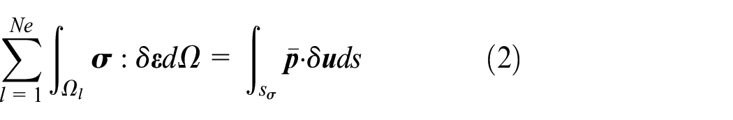
The classical weak form of governing equations for coarse-scale problem or macroscopic problem (without consideration of body force) under quasi-static load are given by

where
where Ne is the amount of material domains in structure and


where Sl is the boundary of material domain

Here, the basic unknowns convert from the displacement defined at every material point to the displacement defined on boundaries of material domains.

Domain information transfer method.
Equation (5) is an important fundament of the proposed DITM. It is easy to prove that the combination of equation (5) and essential boundary condition on
A mesoscopic model with the same size of material domain will be assigned to it to obtain its properties, which replaces the function of operator
The novelty of the proposed method includes the following aspects:
On macroscopic level, material domains are viewed as the elementary substances to construct structure. It is different from the traditional substructure concept because this is the elementary substance with ability to independently reflect both deformation and damage localization phenomenon by itself. The upscaling and downscaling processes are applied to obtain the properties of material domains and corresponding mesoscopic solution is obtained simultaneously. It should be noted that the size of a material domain is not arbitrary. The size should not be too small to reflect macroscopic properties of material. It also should not be too big for the reason that corresponding mesoscopic model needs to be small enough to save computational cost. The governing equations of macroscopic problem are established based on this point of view and the corresponding multi-level domain information transfer mechanism is established to solve the problem.
An IEE is proposed based on nonlocal quadrature scheme which realizes the efficient information transfer between material domain and mesoscopic model.
A kind of damage criterion is established to determine which material domain enters the damage stage. It relates to where the domain information transfer mechanism is activated. So, the computational efficiency is improved significantly.
The boundary displacement of material domain is approximated using IEEs and the damage localization phenomenon is equivalently simulated on macroscopic level, including the phenomenon that the damage localization band gets across boundaries of adjacent material domains.
Discretization on macroscopic level
As basic unknowns on macroscopic level, the boundary displacements of material domains need to be solved. The boundary of each material domain is discretized into several elements, as in macroscopic numerical model depicted in Figure 2. The boundary displacement is interpolated in these elements. Adjacent material domains share the same elements between them. In addition to approximate boundary displacement, the element takes responsibility for information exchange between material domain and mesoscopic model. Thus, it will be called as IEE.

Macroscopic and mesoscopic computational levels.
The size of IEE is a model parameter, which decides the number of degrees of freedom on the boundary of a material domain. Severe deformation mode is allowed somewhere on the material domain’s boundary by reasonable setting of the size of IEE, which makes the equivalent damage localization band to get across the boundary of adjacent material domains. Compared with the concurrent method, the meshes and degrees of freedom of macroscopic model remain unchanged during the analysis, and the load history can be retained, which significantly improves the flexibility and efficiency of the computational framework. The purpose of this article is to establish a computational framework. It shows some advantages in the description of damage localization phenomenon on macroscopic level, but some mesh dependency appears on the boundary of material domain, as discussed in section “Numerical results and discussions.” It will be the future work to deal with the issue.
Benefit from the same basic displacement mode of each IEE, the damage development near material domain’s boundary will not be differentially induced. Without losing generality, linear interpolation is adopted here. The boundary displacement in IEE k can be expressed as

where k is number of IEE,

Here,

where

where


This is the final version of governing equations of macroscopic problem. Here,
Downscaling and mesoscopic computational level
As the explicit representation of operator
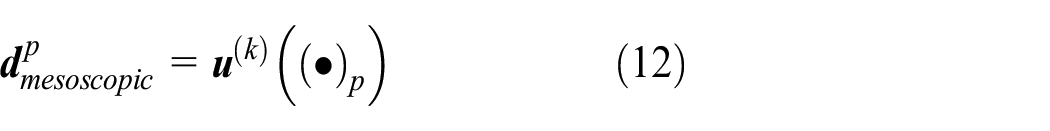
Here,
The solutions of mesoscopic problem will be solved by governing equation (13), which is the governing equation of mesoscopic computational level

where
The tangent stiffness matrix of mesoscopic model is denoted as

gives
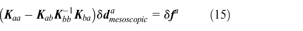
where

The solved boundary nodal forces and condensed tangent stiffness matrix of mesoscopic model will be transferred into macroscopic level for the calculation of domain forces and domain tangent stiffness matrix.
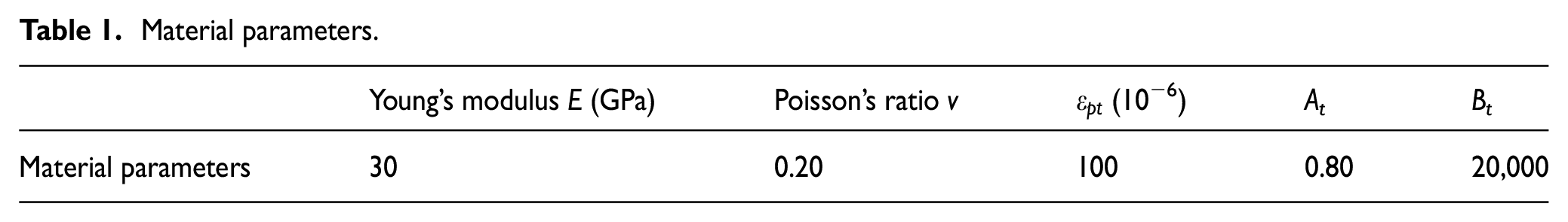
Many types of the mesoscopic models could be adopted to describe the details of material, such as lattice model and FEM. The lattice model is adopted here to establish a mesoscopic model which describes a quasi-brittle material containing distributed initial defects. The model is depicted in Figure 2. The defects are randomly inserted in the model with a relatively uniform and distributed pattern by deleting some of the Lattice elements. The type of mesoscopic element is truss element and model parameters are set according to method mentioned in Guo et al., 50 which will not be narrated here.
The Mazars damage law is adopted to describe the degradation of mechanical property of material in mesoscopic model and the damage caused by compressive stress is ignored. The damage evolution can be expressed as

where

The loading criterion can be

Equation (18) represents the damage surface and
Material parameters.
Quadrature scheme and upscaling
In this section, the IEE based on nonlocal quadrature 52 is proposed and the domain forces and domain tangent stiffness matrix are derived.
The numerical quadrature scheme is necessary to obtain nodal forces of IEE as expressed in equation (8). If Gauss quadrature is adopted, there may not be any mesoscopic node that happens to correspond to the position of quadrature point and the value on Gauss point should be the one with macroscopic meaning. So, it cannot be the same as that one of corresponding mesoscopic node directly. However, the degrees of freedom are usually considerable for mesoscopic model. Therefore, the calculation efficiency of domain forces and domain tangent stiffness matrix should be improved. Here, nonlocal quadrature is applied for that purpose and the IEE with not only quadrature points but also quadrature neighborhood is established.
The nonlocal quadrature of function


where equations (20) and (21) are described in parent element and physical element, respectively.
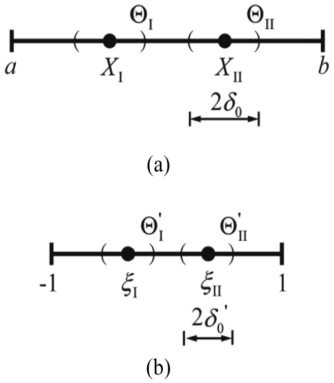
Nonlocal quadrature: (a) physical element and (b) parent element.
Different amount of quadrature points leads to different quadrature parameters. The quadrature parameters of nonlocal quadrature with two quadrature points are
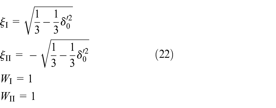
It can be noted that, in a sense, average value of function in the quadrature neighborhood is used as the value on quadrature point, which can smooth local oscillation due to mesoscopic features and obtain a value with macroscopic meaning.
Considering the IEEs shown in Figure 4, each of them contains two quadrature points and corresponding quadrature neighborhoods. The radius
where

IEEs based on nonlocal quadrature.
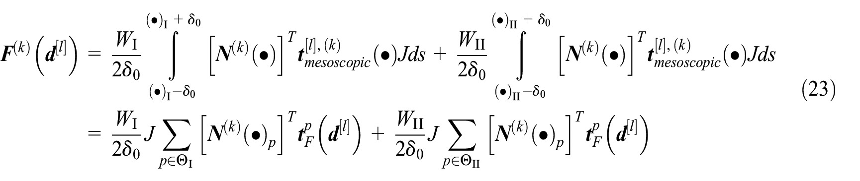
The quadrature weights are same when two quadrature points are adopted. Let
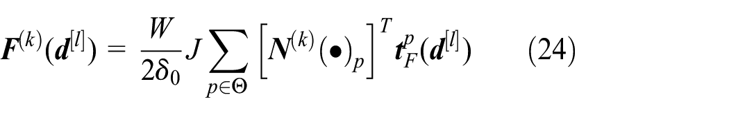
where
Inserting equation (24) into equation (9), which gives domain force
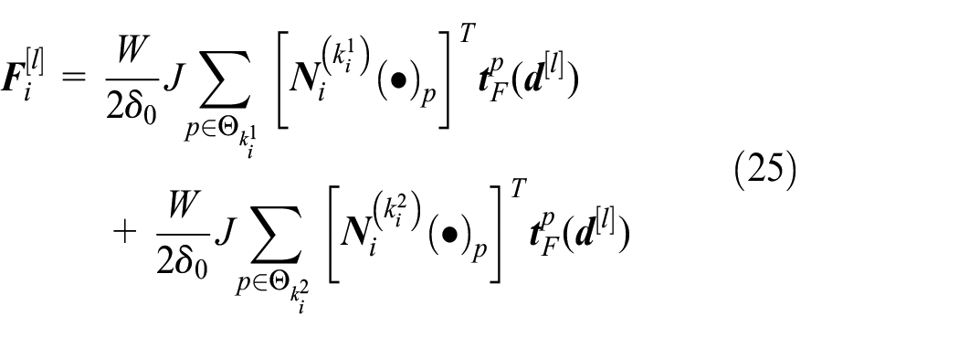
As depicted in Figure 4, node i is a common node of two adjacent IEEs,
In addition to domain forces, domain tangent stiffness matrix will be obtained from mesoscopic level. The domain tangent stiffness matrix of material domain l is denoted as
Here,

and note that i and j are global numbers of domain nodes, and the domain tangent stiffness matrix can be expressed as
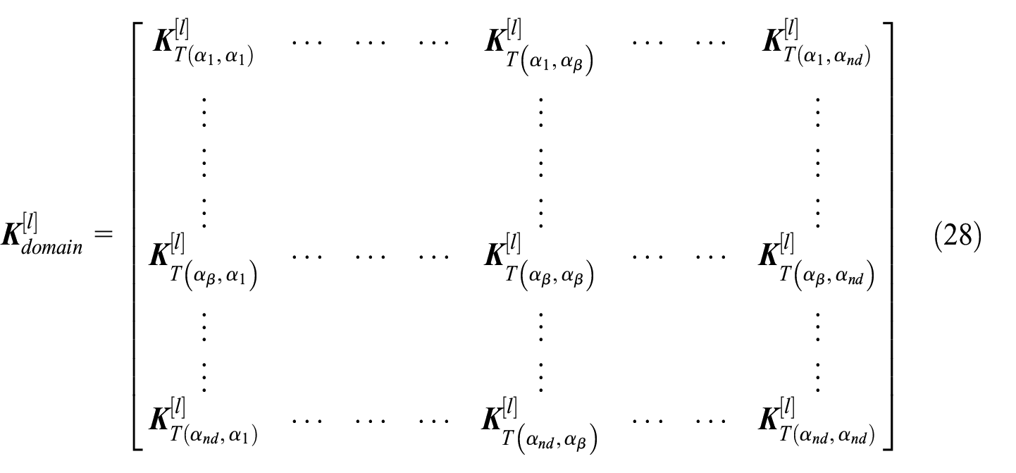
where nd denotes the amount of nodes of a material domain. In macroscopic model,
The domain tangent stiffness matrix reflects the current mechanical properties of material domain and is equivalent to the function of operator

The summation symbol, here, represents the assembly of stiffness matrixes.
Damage criterion and two-level computational framework
The damage criterion of material domain will be described in this section and an efficient two-level computational framework will be established. The mechanical property of intact material domain is assumed to be linear elasticity here.
First, a damage criterion is established based on the deformation of material domain’s boundary. Due to the fact that damage criterion relates to the type of materials and the failure modes of material domain, different damage criterions can be established according to different demands. Here, the failure mode dominated by tensile failure is considered and the boundary strain extremum is defined to establish the damage criterion. For the other failure modes or material types, the damage criterion can also be established according to corresponding characteristics. The boundary strain extremum

where
where
For the intact material domain, the mechanical properties are described by domain elastic stiffness matrix, which is assembled by initial condensed stiffness matrix of corresponding mesoscopic model. The domain elastic stiffness matrix is a constant and obtained by the same way of domain tangent stiffness matrix. The work is completed in pre-analysis step before analysis.
The computational framework is depicted in Figure 5. There are two separated computational levels. The macroscopic problem is divided into several macroscopic load steps and each of them is solved by Newton–Raphson iteration. During the solving process, if the material domain is intact, the response of which will be obtained according to its initial elastic property directly. If the material domain reaches the damage criterion, the domain information transfer mechanism will be activated and the response of that material domain will be obtained from the upscaling and downscaling processes.

Flowchart of domain information transfer method.
It should be noted that the damage criterion is a standard to judge the variation in macroscopic mechanical properties of a material domain, such as the yield surface in plasticity theory. It is not the standard for the substitution of some areas in the model from a macroscopic region to a mesoscopic region. The framework of macroscopic model does not change during the whole analysis. The change exists in the macroscopic properties of material domains. Therefore, different from concurrent method, it is unnecessary to consider the complex variation of the boundary between macroscopic and mesoscopic regions due to damage evolution. However, it realizes the preservation of load history automatically. The load history in the former load steps will not be lost. The variables reflecting load history such as damage variable will be stored in mesoscopic models and be updated after each macroscopic load step. This method saves considerable computational cost because of two main reasons. First, the mesoscopic models will only be assigned to the damaged material domains. Second, load history is preserved automatically so that repeated computation in concurrent method is avoided.
Numerical results and discussions
In this section, results obtained with the DITM are shown and compared with reference solutions obtained by direct numerical simulation (DNS) of the problems. The damage processes of two kinds of specimens consisting of quasi-brittle material are simulated. At mesoscopic level, we consider a quasi-brittle material with initial defects as described in section “Downscaling and mesoscopic computational level.” The DNS model is fully constructed by Lattice elements and its internal structure is periodically repeated by a mesoscopic model (the one assigned to a material domain) with size of 50 mm × 50 mm.
Four-point bending test
For a four-point bending beam subjected to displacement load, the DITM is shown in Figure 6(a). The beam is simply supported. The size of the specimen is 450 mm × 150 mm. The problem is simplified to a plane problem and the result of the sum of reaction forces at loading position is expressed as the force acting on unit thickness. In DITM, the investigated specimen consists of 27 material domains. There are 608 degrees of freedom and 330 IEEs on the boundaries of material domains in the structure. The corresponding DNS for the same problem has 1,36,202 degrees of freedom. The size of each material domain is 50 mm × 50 mm and IEEs with size of 10 mm are applied. Considering the area near mid-span is the main damage region that should be concerned, the damage of domains (16) and (27) which are close to supports is ignored.

(a) The four-point bending beam modeled by DITM and (b) force displacement curves obtained from DITM and DNS.
The calculated force–displacement curves of DITM and DNS are plotted in Figure 6(b). One can see that DITM result agrees well with the DNS analysis. The damage contours at the end of analysis obtained from DITM and DNS are depicted in Figure 7. The damage pattern obtained from DITM is in relatively good agreement with the one obtained from DNS. It should also be noted that the damage profiles obtained by DITM suggest some spurious damage localization at the horizontal edges of the material domains. It shows some mesh dependency here. One reason is that the size of IEE restricts the range of damage area near it. The deformation along the direction of an IEE is similar; so, the damage is similar there, which results in the range of damage area near IEE close to the size of IEE when damage localization happens. Another reason is that the nonlocal interaction does not extend in the transverse direction of IEE although the nonlocal quadrature is adopted. It is should be pointed out that the damage contours obtained from DITM are results on mesoscopic computational level, assembled by each damaged material domain. The material domains which do not meet damage criterion are also described in Figure 7(a) to construct the whole specimen for the comparison of DITM and DNS results.

Damage contours obtained from (a) DITM and (b) DNS at the end of analysis.
Figure 8 shows the damage evolution process obtained from DITM. The contours describe the whole process from distributed damage-to-damage localization phenomenon. The damage patterns a–h correspond to reference points a–h depicted in force–displacement curve. The right superscript of each contour indicates the number of damaged material domain. The amount of damaged material domains corresponding to each reference point increases with the continuous increase of displacement load. It should be noted that during the procedure between points a and b, damage distributes around the defects over the bottom of specimen near mid-span areas. The damage localization zone occurs at point c, the peak load. After that, it bifurcates into two main damage localization zones which develop simultaneously. These two damage localization zones coalesce into one at point g and form the obvious damage localization band in the specimen. After point h, the damage localization band penetrates the specimen and results in its failure. It can be seen that damage localization band gets across three material domains and makes the damaged material domains beside these three ones unloaded, which stops the damage evolution there.

Damage evolution in material domains.
During the DITM analysis, domain information transfer mechanism is activated at six material domains sequentially as plotted in Figure 9. Each subfigure corresponds to a point marked in the force–displacement curve as shown in Figure 9. It shows that up to point a, all of the material domains are intact. With damage evolution, the damaged material domains appear from bottom to top of the specimen. One can see that only the areas near mid-span are damaged while other areas retain intact during analysis.

Activation procedure of domain information transfer mechanism at material domains.
On macroscopic level, the specimen deformation obtained from DITM at the end of analysis is shown in Figure 10. It can be noted that the deformation of most of material domains is relatively small except for three material domains located on mid-span areas. On the locations where damage localization band gets across the boundaries of adjacent material domains, the deformation is obviously larger than that of other locations on material domains’ boundaries, which indicates the local cracking here. It should be noted that the phenomenon of local failure is described on macroscopic level by local severe deformation of boundaries of material domains. In this method, when and where the damage localization band will generate is solved by DITM automatically. The locations where damage localization band gets across boundaries of adjacent material domains are also obtained automatically. It makes it unnecessary to consider how to insert an equivalent damage localization band (including its length, direction, and pattern) into macroscopic element at proper instant, to represent local failure under hierarchical computational framework. The boundary deformation can represent damage pattern of a material domain containing damage localization band such as domains (2), (5), and (8) in Figure 10. It can be seen that domains (5) and (8) are penetrated by damage localization band while domain (2) is not penetrated totally. According to the deformation pattern of damaged material domains, the region of damage localization band can be located in macroscopic model. One should note that it is a new way to equivalently represent the damage localization band on macroscopic level. Simultaneously, the effect of the failure region on the overall performance of structure is precisely reflected by the mechanical properties of material domains which contain them. If the exact pattern of damage localization band needs to be seen, the result obtained from mesoscopic level in DITM can be assembled to show the pattern, such as shown in Figure 10. (The contours here are fracture contours and the mesoscopic elements with damage value of 1.0 are identified in contours.)

Specimen deformation on macroscopic level (magnified 200 times) and corresponding mesoscopic fracture pattern obtained from DITM at the end of analysis.
Cantilever beam test
A cantilever beam subjected to a uniform vertical load on its right side is analyzed by DITM and DNS. The material domain is the same as applied in section “Four-point bending test.” The DITM of the specimen with size of 250 mm × 100 mm is depicted in Figure 11(a). The model consists of 10 material domains. The calculated force–displacement curves obtained from DITM and DNS are shown in Figure 11(b). One can see that the DITM result is in relatively good agreement with the DNS analysis result with respect to both the slope of the linear part and the trend of the softening branch. The difference in the peak load is due to coarse-scale discretization of material domain’s boundary. The damage patterns obtained from DITM and DNS at the end of analysis are compared as shown in Figure 12. It can be noted that the DITM result agrees well with DNS analysis result except for some locations in the horizontal edges of the material domains, which shows some mesh dependency as mentioned in section “Four-point bending test.”

(a) The cantilever beam modeled by DITM and (b) force displacement curves obtained from DITM and DNS.

Damage contours obtained from (a) DITM and (b) DNS at the end of analysis.
The damage evolution in material domains obtained from DITM is shown in Figure 13. It can be seen that between points a and b, damage is distributed near the upper left end of the specimen, where the tensile stress is relatively high. The damage develops in domains (1) and (2) along lengthwise direction of specimen at first, while damage localization band generates and develops after point c, material domain (2) is unloaded and the damage evolution stops there. At point e, the damage localization band gets across the boundary of domains (1) and (6) and enters into domain (6). It develops until the specimen is almost penetrated as plotted in subfigure g.
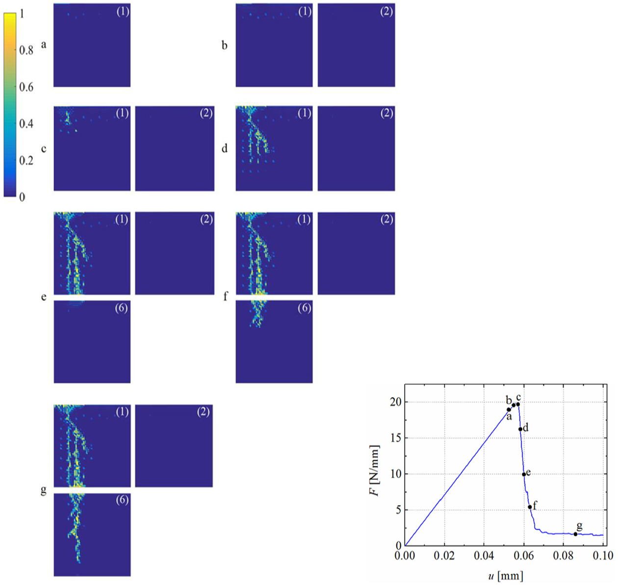
Damage evolution in material domains.
The domain information transfer mechanism is activated at only three material domains during the DITM analysis, as depicted in Figure 14. One can note that up to point a, all the material domains are intact. The activation process and locations of damaged material domains are in consistent with the damage evolution process in Figure 13.

Activation procedure of domain information transfer mechanism at material domains.
The specimen deformation on macroscopic level obtained from DITM at the end of analysis is shown in Figure 15. It is obvious that domain (1) is penetrated by the damage localization band in the left side of it. The severe deformed IEEs on the two horizontal boundaries of this material domain indicate the locations where the damage localization band gets across material domains’ boundaries. It should be noted that the location of the damage localization band in a material domain can be simulated accurately.

Specimen deformation on macroscopic level (magnified 200 times) and corresponding mesoscopic fracture pattern obtained from DITM at the end of analysis.
Computational cost comparison
As the initial elastic property is pre-analyzed and assigned to each material domain, the responses of material domains are computed directly according to such property before they meet damage criterion. It saves considerable computational cost. In addition, it is not required to specify where the mechanism should be activated before analysis. In the four-point bending test problem, 6 material domains of the total 27 material domains are activated with the domain information transfer mechanism (≈22%). For the cantilever beam test problem, 30% of the material domains are activated with the domain information transfer mechanism. One should note that the domain information transfer mechanism is activated sequentially, which keeps a relatively lower computational cost before the specimen approaching failure. With the same computational resources, the total computational time of DITM and DNS of the four-point bending test problem are 8 and 60 h, respectively, as plotted in Figure 16. It takes 3 and 26 h of the cantilever beam test problem for DITM and DNS, respectively. Here, models 1 and 2 refer to four-point bending specimen and cantilever beam specimen, respectively. It can be seen that the computational cost saving is significant by DITM.

Computational cost comparison between DITM and DNS.
Conclusion
The DITM is proposed in this article for the purpose of quasi-brittle failure analysis. It contains two separated computational levels. On macroscopic level, the material domains are viewed as elementary substances which construct the whole structure. The macroscopic governing equations are established based on this point of view and boundary displacement of material domains are defined as basic unknowns. Each damaged material domain will be assigned a mesoscale model and the information transfer mechanism from a mesoscale domain to a macroscale domain is established. The damage localization phenomenon is equivalently represented on macroscopic level by boundary deformation of material domains. Simultaneously, details of damage pattern are obtained from mesoscopic level. The IEE based on nonlocal quadrature scheme is proposed and the efficient upscaling is realized by this type of element.
The numerical results show that the proposed method can properly predict the damage pattern and describe the process form distributed damage-to-damage localization. While, it seems to be some mesh dependency with the size of IEE. Also, if the size of material domain will affect the simulation results or if there is a proper value of the size are still an important issue to be studied. Further research will be conducted to solve the problems mentioned here.
Footnotes
Appendix 1
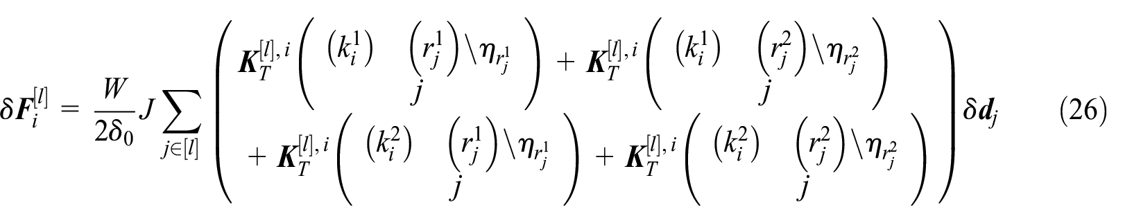
The domain tangent stiffness matrix will be detailed here and the meaning of stiffness assembly symbol in equation (26) will be explained.
The variation in traction of node p on the boundary of mesoscopic model is
where
Defining
where
Here,
Acknowledgements
The authors are very grateful to editors and reviewers for carefully reading the paper and for their comments and suggestions.
Handling Editor: James Baldwin
Declaration of conflicting interests
The author(s) declared no potential conflicts of interest with respect to the research, authorship, and/or publication of this article.
Funding
The author(s) disclosed receipt of the following financial support for the research, authorship, and/or publication of this article: This work was supported by the National Natural Science Foundation of China (Nos 51878154, 51578142, and 51478108).