Sage Journals: Discover world-class research

Abstract

The mold is referred to as the heart of the continuous casting machine. Mold-level control is one of the keys to ensuring the quality of a high-efficiency continuous casting slab. This article addresses the failure of the mold-level prediction model in the actual production process to overcome the impact of noise. To improve the accuracy of mold-level prediction, a novel method for mold-level prediction based on the multi-mode decomposition method and the long short-term memory model is proposed. First, empirical mode decomposition of the mold-level data is performed. The actual eigenmode component number K is obtained through the calculation of the mutual information entropy of the eigenmode components. Then, we perform a K-based variational mode decomposition on the mold-level data. The noise dominant component is denoised by the calculation of the mutual information entropy of the eigenmode components. Moreover, the long short-term memory model is used to predict the noise dominant component and the information dominant component after denoising. Finally, the predicted result is subjected to variational mode decomposition reconstruction to obtain the predicted mold-level data. The experimental results show that compared with the other methods tested, the model has better prediction efficiency, prediction accuracy, and generalization ability. It provides a new idea for mold-liquid-level prediction and continuous casting blank quality assurance.

Keywords

Multi-mode decomposition long short-term memory model mutual information entropy continuous casting mold level

Introduction

The mold is referred to as the heart of the continuous casting machine.¹ Mold-level control is the basis for stable production operations, avoiding steel leakage and steel spillage. The fluctuation of the mold level is disturbed by many factors.² It has the characteristics of nonlinearity, variation with time, and uncertainty. These manifest as many disturbances in production operations, such as sudden-speed abrupt changes and time-varying and nonlinear disturbances in the sliding nozzle due to wear and clogging. The mold-level model is shown in Figure 1.

Figure 1.

Mold-level model.

Accurate mold-level control is a key factor in ensuring the quality of the slab. It is an important reference for speed control, roll gap control, mold secondary cooling water control, and plug control. During the continuous casting process, fluctuations in the mold level cause many problems. If the mold level fluctuates too much, first it will cause impurities on the surface of the mold. Surface defects and internal defects of the slab are generated, which affect the surface and internal quality of the slab. Second, it will affect the casting speed, affecting productivity and the production rhythm. Eventually, it will cause the slab and the continuous casting machine to stick together, damage the tundish slide, and even cause downtime. Accurate prediction of the mold level thus occupies an important position in the continuous casting production process.

In order to maintain the stability of the mold level, many scholars have conducted research on mold-level control in recent years. The main methods are proportional–integral–differential (PID) control, fuzzy control, adaptive control, and so on. M Dussud et al.³ developed a fuzzy controller based on expert knowledge for process control when the mold level is disturbed. In Hesketh et al.,⁴ an adaptive controller was applied to control the mold level. The controller was embedded in a real-time control program based on a PC. It combines the filter, noise model, and other technologies and provides a new method for the control of the mold level. In De Keyser,^5,6 the results of applying model predictive control to mold-level control were presented and compared with standard PID control. The results showed that model predictive control can improve the accuracy of mold-level control. In Kong et al.,⁷ different adaptive predictive control methods for online parameter identification were simulated and studied. The advantages and disadvantages of the adaptive predictive method and the standard PID controller were compared. Mold-level prediction is often used to regulate the flow of liquid steel in the continuous casting line part of the process of making steel. K Dekemele et al.⁸ proposed a novel inferential control strategy; this work improved the current operation and indicated that real plant implementation is feasible. D Copot et al.⁹ proposed a fractional-order control design with adaptive laws. A real-time embedded control setup and interface to industrial standard devices was tested to illustrate the implementation aspects of the proposed fractional-order control. Traditional mold-level control uses methods such as neural networks and generalized prediction. However, the continuous casting production process is a strong coupling and nonlinear process with many interference signals, which leads to a decrease in prediction accuracy, and these methods thus cannot meet the requirements of continuous casting production.

In recent years, signal processing methods have developed by leaps and bounds, and many scholars have conducted extensive research on the prediction of time series. In 1998, Huang et al.¹⁰ proposed empirical mode decomposition (EMD). EMD is an adaptive decomposition method without a prior matrix.¹¹ Since the introduction of EMD by Huang, it has been widely used in the biomedical,^12,13 speech recognition,¹⁴ system modeling,^15–17 and process control^18,19 fields. In recent years, a new signal processing method called the variational mode decomposition (VMD) technique has enriched the signal denoising method. K Dragomiretskiy and D Zosso²⁰ proposed a VMD method. VMD is a completely nonrecursive VMD model. It finds the center frequency and bandwidth of each decomposition component by iteratively searching for the optimal solution to the variational model, adaptively splits the frequency domain of the signal, and effectively separates the components. Compared with the EMD method, VMD effectively avoids mode aliasing and boundary effects, adaptively implements frequency-domain splitting and effective separation of components, and has better noise and sample rate robustness. Y Zhang et al.²¹ proposed short-term wind power prediction based on a quantile regression average and a VMD-based hybrid model. S Lahmiri²² proposed a method for signal denoising combined with VMD and discrete wavelet transform.

Recurrent neural networks (RNNs) are deep learning neural networks that differ from traditional feedforward neural network (FNN). Introducing directional loops into the RNN structure enables the extraction of associated information in the sequence data and is widely used in fields such as natural language processing due to its superiority in processing sequence data. However, if there is a long-term dependency between the samples, there will be a gradient disappearance problem. Long short-term memory (LSTM) is an improved neural network for this problem. The LSTM neural network was proposed by Hochreiter and Schmidhuber²³ and improved by Graves et al.²⁴ There are three gates in the LSTM neuron structure, namely, the input gate, output gate, and forget gate, which are used to filter useful information from historical data. LSTM-based systems can learn language translation,^25,26 robot control,^27,28 image recognition,^29,30 and so on.

VMD is an excellent signal decomposition method. Compared with EMD, VMD has a complete mathematical theory basis and has no pattern aliasing and boundary effects inherent. Combined with the adaptive decomposition characteristics of EMD, the VMD method is improved. The method proposed in this article no longer requires prior knowledge compared to the wavelet transform (WT) method. LSTM is a time series prediction method based on the deep learning computing framework. Compared with the traditional support vector machine (SVR), the prediction efficiency is higher and the prediction accuracy is better. Therefore, this article studies the time series prediction performance of the hybrid methods of VMD and LSTM.

This article mainly combines multi-mode decomposition (MMD) and LSTM to predict the mold level. First, the mold level is decomposed by EMD, and the eigenmode component number K is obtained by calculating the mutual information entropy (MIE) of the intrinsic mode functions (IMFs). Second, the mold-level data are decomposed based on the K-based VMD. The high-frequency and the low-frequency IMF boundaries are obtained by calculating the MIE of the eigenmode component, and wavelet threshold denoising (WTD) is performed on the high-frequency IMFs to provide denoising. Finally, the LSTM model predicts the processed IMFs, and the prediction result is reconstructed to obtain the predicted mold level. The layout of this article is as follows: The second section introduces VMD, LSTM, and MIE. The third section introduces the MMD-LSTM model. The fourth section compares the results of various methods. The fifth section discusses the results. Finally, our conclusion is presented.

Basic algorithms

The basic principle of VMD

VMD is a new type of signal decomposition method. This method redefines an AM–FM (amplitude modulation–frequency modulation) signal as an eigenmode component. Its expression is

u_{k} (t) = A_{k} (t) 2 \cos (f_{k} (t))

(1)

where phase ϕ_k(t) is a nondecreasing function, A_k(t) is the instantaneous amplitude of u_k(t), and A_k(t) ≥ 0. ω_k(t) = ϕ′_k(t), which is the instantaneous frequency of u_k(t).

In the interval range of [t − δ, t + δ], u_k(t) can be regarded as a harmonic signal with amplitude A_k(t) and frequency ω_k(t), and $δ = 2 π / f'_{k} (t)$ .

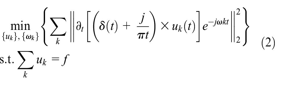
The difference between VMD and EMD is that VMD is based on solving the variational problem. In the process of obtaining eigenmode components, the variational model principle is used to minimize the sum of the estimated bandwidths of each eigenmode component. The optimal solution of the constrained variational model is found. The center frequency and bandwidth of the eigenmode component are updated in the process of solving the variational model. The signal band is adaptively segmented based on the frequency domain of the signal itself. Furthermore, a narrow-band eigenmode component is obtained.

The variational constraint model is as follows

\begin{matrix} min_{{u_{k}}, {ω_{k}}} {\sum_{k} {‖ \partial_{t} [(δ (t) + \frac{j}{π t}) \times u_{k} (t)] e^{- j ω kt} ‖}_{2}^{2}} \\ s . t . \sum_{k} u_{k} = f \end{matrix}

(2)

where ${u_{k}} : = {u_{1}, u_{2}, \dots, u_{K}}$ represents K-many IMFs, ${ω_{k}} : = {ω_{1}, ω_{2}, \dots, ω_{K}}$ represents the frequency center of each IMF, and $\sum_{k} : = \sum_{k = 1}^{K}$ represents the sum of all modes.

We introduce the Lagrange function as

\begin{matrix} L ({u_{k}}, {ω_{k}}, λ) = α \sum_{k} {‖ \partial_{t} [(δ (t) + \frac{j}{π t}) \times u_{k} (t)] e^{- j ω kt} ‖}_{2}^{2} \\ + ‖ f (t) - \sum_{k} u_{k} (t) ‖_{2}^{2} + 〈 λ (t), f (t) - \sum_{k} u_{k} (t) 〉 \end{matrix}

(3)

where α is the penalty factor, λ is the Lagrange multiplier, and $‖ f (t) - \sum_{k} u_{k} (t) ‖_{2}^{2}$ is the second penalty.

The problem of solving the original minimum value can be transformed into the saddle point of the extended Lagrange expression by the alternating direction method; this is the optimal solution of the above formula

u_{k}^{n + 1} = \arg_{uk} min L ({u_{i < k}^{n + 1}}, {u_{i \geq k}^{n + 1}}, {ω_{i}^{n}}, λ^{n})

(4)

ω_{k}^{n + 1} = \arg_{ω k} min L ({u_{i}^{n + 1}}, {ω_{i < k}^{n + 1}}, {ω_{i \geq k}^{n}}, λ^{n})

(5)

λ^{n + 1} = λ^{n} + τ (x - \sum_{k} u_{k}^{n + 1})

(6)

where $\sum_{k} ‖ u_{k}^{n + 1} - u_{k}^{n} ‖_{2}^{2} / ‖ u_{k}^{n} ‖_{2}^{2} < ε$ is the convergence condition and n is the number of iterations.

Therefore, the original signal can be decomposed into K IMFs.

The calculation process of the VMD algorithm is as follows:

Step 1. Initialize ${u_{k}^{1}}$ , ${ω_{k}^{1}}$ , $λ^{1}$ , and n to zero;

Step 2. n = n + 1, execute the entire loop;

Step 3. Execute the loop k = k + 1 until k equals k, then update $u_{k} : u_{k}^{n + 1} = \underset{u_{k}}{\arg min L} ({u_{i < k}^{n + 1}}, {u_{i \geq k}^{n}}, {u_{i}^{n}}, λ^{n})$ ;

Step 4. Execute the loop k = k + 1 until k equals K, then update $ω_{k} : ω_{k}^{n + 1} = \underset{ω_{k}}{\arg min L} ({ω_{i < k}^{n + 1}}, {ω_{i \geq k}^{n}}, {ω_{i}^{n}}, λ^{n})$ ;

Step 5. Use $λ^{n + 1} = λ_{n} + τ (f (t) - \sum_{k} u_{k} (t))$ to update λ;

Step 6. Given the discrimination condition ε > 0, if the iteration stop condition is satisfied, all the cycles are stopped and the result is output, and K IMFs are obtained.

The basic principle of LSTM

In the LSTM neuron structure shown in Figure 2, let x = [x₁, x₂, x₃, …, x_t] be the input timing signal and x_t be the input of the neuron at time t. Let y = [y₁, y₂, y₃, …, y_t] be the corresponding output target and y_t be the output at time t. Let c = [c₁, c₂, c₃, …, c_t] represent the state information of the neuron and c_t be the state matrix of the neuron at time t. Then, the LSTM memory unit calculation process can be expressed as follows

i_{t} = sig (w_{i} \cdot [y_{t - 1}, c_{t - 1}, x_{t}] + b_{i})

(7)

f_{t} = sig (w_{f} \cdot [y_{t - 1}, c_{t - 1}, x_{t}] + b_{f})

(8)

o_{t} = sig (w_{o} \cdot [y_{t - 1}, c_{t - 1}, x_{t}] + b_{o})

(9)

μ_{t} = sig (w_{μ} \cdot [y_{t - 1}, c_{t - 1}, x_{t}] + b_{μ})

(10)

Figure 2.

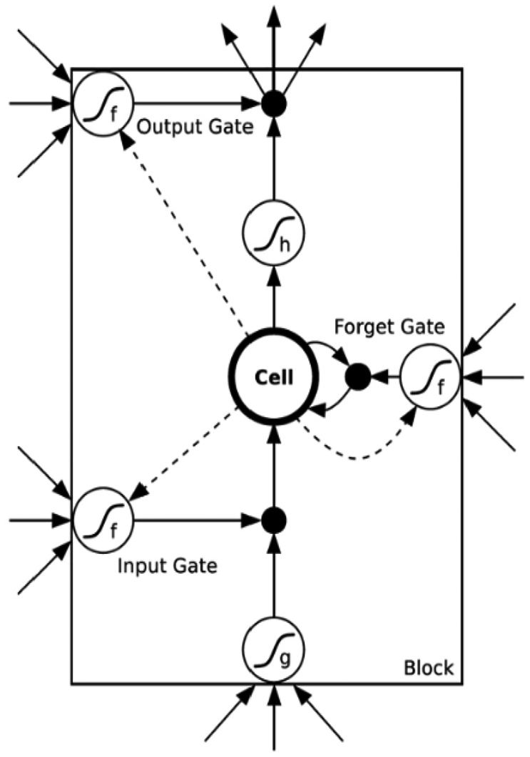
The long short-term memory (LSTM) block structure.

In these formulas, w_i, w_f, w_o, and w_μ represent the input gate, forget gate, output gate, and neuron state matrix in the neuron structure, respectively; b_i, b_f, b_o, and b_μ represent the corresponding offset constants; and sig(·) represents the sigmoid function.

According to the formula above, the LSTM neuron structure expression in Figure 2 of the neuron state c_t and the output y_t is as follows

c_{t} = f_{t} \otimes {c_{t}}_{- 1} + i_{t} \otimes μ_{t}

(11)

y_{t} = o_{t} \otimes \tanh (c_{t})

(12)

where ⊗ represents matrix point multiplication.

MIE

After VMD decomposition, the mold-level signal s(t) can be expressed as

s (t) = \sum_{i = 1}^{n} S_{IM F_{i}} (t) + r_{n} (t)

(13)

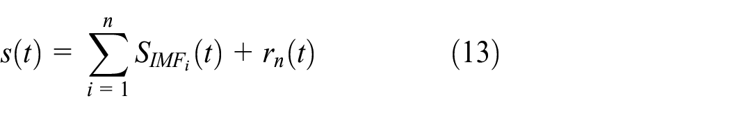
where S_IMFi(t) represents the IMF, the frequency of which is ranked from high to low and r_n(t) represents the residual, representing the average trend of the signal. We modify equation (1) to

s (t) = H (t) + L (t)

(14)

where $H (t) = \sum_{i = 1}^{k - 1} S_{IM F_{i}} (t)$ represents the IMF combination of the high-frequency components and $L (t) = \sum_{i = 1}^{n} S_{IM F_{i}} (t) + r_{n} (t)$ represents the IMF and residual combination of the low-frequency components.

MIE is used to measure the statistical dependence between two random variables. Its expression is $I (X, Y) = \sum_{i = 1}^{r} \sum_{j = 1}^{s} p (x_{i}, y_{i}) lb (p (x_{i}, y_{i}) / p (x_{i}) p (y_{i}))$ , where p(x_i, y_i) is the joint probability distribution, p(x_i) and p(y_i) are the edge probability distributions, X and Y represent different IMFs, and the r and s distributions represent the number of symbols of X and Y, respectively.

If the high-frequency component is noise interference and the low-frequency component is an effective signal, the MIE relationship between the IMFs can be used to identify the boundary between the high-frequency and low-frequency components. The IMF characteristics obtained by the VMD show that the dependence of the high-frequency noise on each IMF is gradually reduced, and the dependence of the low-frequency effective signal on each IMF is gradually enhanced. Therefore, it can be assumed that the high-frequency component and the low-frequency component are partially statistically independent of each other. It is known from the characteristics of MIE that the MIE between two independent random variables should be equal to 0. Therefore, when calculating the MIE between each adjacent IMF, a local minimum value occurs, and only the first local minimum value is searched to obtain a boundary between the high-frequency component and the low-frequency component. Thus, the following search objective function can be obtained

k = first {min_{1 \leq i \leq n - 1} [I (S_{IM F_{i}}, S_{IM F_{i + 1}})]}

(15)

where k is the high-frequency component, and the low-frequency component is decomposed into the IMF serial number.

Mold-liquid-level prediction based on MMD-LSTM

Since the mode number of the original signal decomposition in the VMD algorithm is an a priori knowledge estimation, there is a certain randomness which may lead to error in mode decomposition. Based on the characteristics of EMD adaptive decomposition, the original signal is decomposed, and the MIE between the IMFs is analyzed to determine the effective mode number K.

The single-mode decomposition method has a certain denoising effect on the signal-to-noise separation of noise signals, but there are also various problems that may lead to the loss of effective information and incomplete noise removal. In this article, the denoising algorithm of the hybrid method is proposed, and the noise dominant component generated by single-mode decomposition is further denoised so that the signal is separated from the noise and the effective information is retained as much as possible. In addition, the algorithm can improve the denoising effect and performance indicators of the mode decomposition method.

Although the traditional prediction algorithm can perform simple prediction, the prediction accuracy is low, the robustness is poor, and the prediction requirements of nonlinear and non-Gaussian distributed data cannot be met. The advanced LSTM algorithm proposed in this article is used to predict the time series of IMF, which can improve the accuracy of prediction and the generalization ability of the model. The MMD-LSTM flowchart is shown in Figure 3. The steps of the MMD-LSTM algorithm are shown in Table 1.

Figure 3.

Multi-mode decomposition (MMD)-LSTM flowchart.

Table 1.

MMD-LSTM algorithm steps.

Step 1. Decompose the original signal into multiple IMFs using EMD.

Step 2. Calculate MIE between IMFs after EMD decomposition, and determine the K value.

Step 3. Perform K-based VMD of the original signal to obtain K-many IMFs.

Step 4. Calculate MIE between IMFs after VMD decomposition, determine noise IMFs, and clear signal IMFs.

Step 5. Perform WTD on the noise-domain IMFs to obtain noise-domain IMFs after denoising.

Step 6. Perform LSTM prediction on all the processed IMFs to obtain the predicted IMFs.

Step 7. Reconstruct the signal with the predicted IMFs to obtain the predicted signal.

MMD: multi-mode decomposition; LSTM: long short-term memory; IMF: intrinsic mode function; EMD: empirical mode decomposition; MIE: mutual information entropy; VMD: variational mode decomposition; WTD: wavelet threshold denoising.

Test analysis

Data source

In order to express the applicability, superiority, and generalization capability of the model application clearly, mold-level data of actual process parameters collected from the continuous casting machine developed by the China National Heavy Machinery Research Institute Co., Ltd (Xi’an, China) are used in this article. There are many uncertain disturbance factors in the control process of the mold level, and the disturbance may change constantly at any time. Most of the disturbances are nonlinear and nonstationary, and the long-term prediction model is difficult to establish. This article asserts that a mold-level prediction model is important for mold-level control to propose new ideas to improve continuous casting automatic control.

A continuous casting production process data acquisition graph is presented in Figure 4. The time interval Δt = 0.5 h and the sampling frequency is 3 Hz.

Figure 4.

Mold level.

The main technical parameters of the continuous casting machine are shown in Table 2.

Table 2.

Main technical parameters of the continuous casting machine.

Project	Specification
Continuous casting machine model	Curved continuous caster
Secondary cooling category	Aerosol cooling, dynamic water distribution
Gap control	Remote adjustment, dynamic soft reduction
Basic arc radius (mm)	9500
Mold length (mm)	900
Metallurgical length (mm)	39,200
Mold vibration frequency (times/min)	25–400
Mold vibration amplitude (mm)	2–10
Slab width (mm)	900–2150
Slab thickness (mm)	230/250
Working speed (m/min)	0.8–2.03

MMD-LSTM-based mold-liquid-level prediction

First, the mold-liquid-level data were EMD decomposed, as shown in Figure 5.

Figure 5.

Mold-level decomposition results by EMD.

As shown in Table 3 and Figure 5, the MIE of IMF (2–3) was 0.7567, which was the first local minimum MIE between IMFs by EMD, so IMF3 is the boundary line between high-frequency IMFs and low-frequency IMFs. The high-frequency IMFs were seen as a mode, while the other IMFs were seen as different modes separately, and we determined that K = 9. The mold-level signal was decomposed using VMD based on K = 9.

Table 3.

MIE between IMFs by EMD.

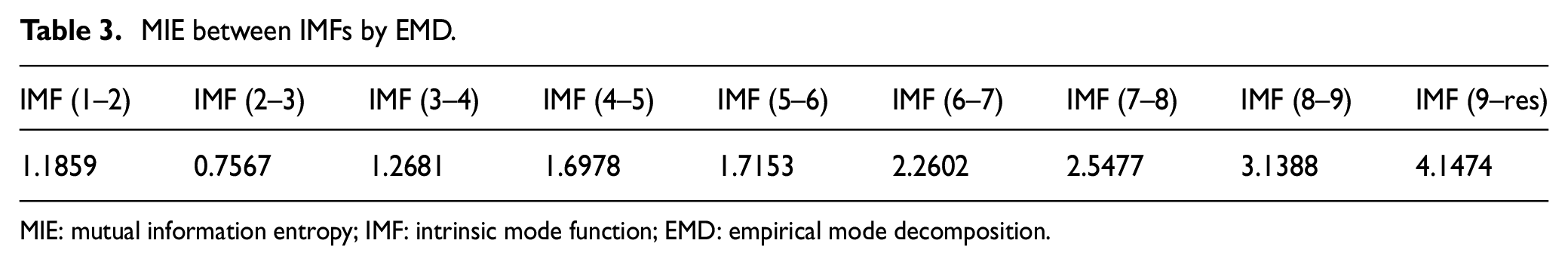
IMF (1–2)	IMF (2–3)	IMF (3–4)	IMF (4–5)	IMF (5–6)	IMF (6–7)	IMF (7–8)	IMF (8–9)	IMF (9–res)
1.1859	0.7567	1.2681	1.6978	1.7153	2.2602	2.5477	3.1388	4.1474

MIE: mutual information entropy; IMF: intrinsic mode function; EMD: empirical mode decomposition.

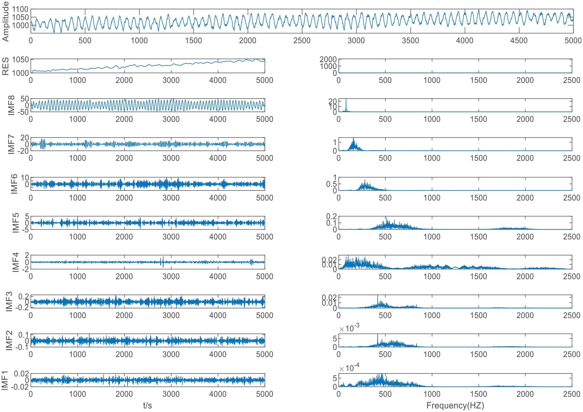
As shown in Table 4 and Figure 6, the MIE of IMF (4–5) is 1.4114, which is the first local minimum MIE between the IMFs by VMD, so IMF5 is the boundary line between the high-frequency IMFs and the low-frequency IMFs; thus, we performed WTD denoising on the first five IMFs.

Table 4.

MIE after VMD.

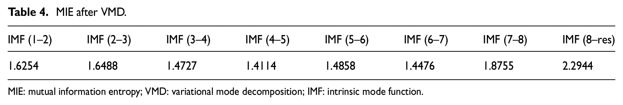
IMF (1–2)	IMF (2–3)	IMF (3–4)	IMF (4–5)	IMF (5–6)	IMF (6–7)	IMF (7–8)	IMF (8–res)
1.6254	1.6488	1.4727	1.4114	1.4858	1.4476	1.8755	2.2944

MIE: mutual information entropy; VMD: variational mode decomposition; IMF: intrinsic mode function.

Figure 6.

Mold-level data VMD results.

As shown in Figure 6, by selecting K = 9 as the mode component number for VMD decomposition, we were able to clearly separate the original signals and avoid modal aliasing. It can be seen from the spectrum diagram that the IMF3–IMF7 frequency bandwidth is relatively long and the noise is serious, so WTD was performed on these IMFs.

As shown in Figure 7, the first five IMFs’ center frequencies were significantly reduced and the amplitudes were also significantly reduced.

Figure 7.

Wavelet threshold denoising (WTD) results of IMF1–IMF5.

It can be seen from Figure 7 that the IMFs after WTD have a more pronounced center frequency and a much narrower frequency band. IMF1–IMF5 and the other IMFs after WTD were reconstructed using VMD to obtain the denoised signal. This method had a good denoising effect and effectively retained the effective information of the original signal.

The LSTM prediction was performed on each IMF, and the predicted IMFs were obtained and reconstructed.

As shown in Figure 4, the collected time series contained 5000 points. On the basis of normalizing the original data, the training set, validation set, test set, and their labels and samples were divided.

We selected a window of length A and segmented it from the data origin. Each segmentation can produce a continuous time series with length A. Each time the segmentation is completed, the window slides n points to the right for the next segmentation. When the length of the remaining data is less than A, the sliding stops. The experimental results show that the network accuracy and efficiency are best when A is 20 and n is 1. After segmentation, 4981 continuous time series of length 20 were obtained. The last one of each sequence was the label value and the first 19 were the sample values, and the original data set was established based on them.

Of the data in the data set, 90% were used as training data to train the network, and the remaining 10% were used as a test set to test the performance of the network. In order to control and adjust the parameters in the training process, data from the training set (10% of the total data) were used as a verification set. The sizes of the training set, verification set, and test set were as follows:

Training set: (4033, 19, 1);

Verification set: (449, 19, 1);

Test set: (499, 19, 1).

The basic structure of the network is shown in Figure 8. The first layer of LSTM contained 128 neurons with 66,560 parameters, and the second layer contained 256 neurons with 394,240 parameters. In order to reduce the dimension of the output results, Linear was used as the activation function in both LSTM layers. Then, we connected the Dropout layer and set its rate to 0.5 to prevent overfitting and to improve the network generalization ability. Finally, the full connection layer was connected to make the output be 1, that is, to achieve single-step prediction. This layer contained 257 parameters, and the total number of parameters of the network was 461,057. Mean square error (MSE) was selected as the loss function, the more efficient Root Mean Square Prop was selected as the optimization operator to accelerate the learning of the network, and the initial learning rate was set at 0.001.

Figure 8.

Basic structure of LSTM.

We set the amount of training data for each batch to 50, and the final validation and training curve stabilized to the lowest value when the epoch number reached 100. The training time was about 610.3 s.

The construction and training of the neural network was based on the Keras framework with Tensorflow as the back end.

The detailed structural parameters of LSTM are shown in Table 5.

Table 5.

Detailed structural parameters of LSTM.

Layers	Layer names	Output shapes	Main parameters of layers	Number of trainable parameters	Other parameters
1	LSTM	(None, 19, 128)	Unit = 128	66,560	Activation = Linear, return_sequences = True
2	LSTM	(None, 256)	Unit = 256	394,240	Activation = Linear, return_sequences = False
3	Dropout	–	–	0	Rate = 0.5
4	Dense	(None, 1)	Unit = 1	257	–
				Total = 461,057

LSTM: long short-term memory.

In Figure 9, there is a comparison between the VMD-LSTM-predicted mold-level data and the actual mold-level data. As shown in Figure 10, in the mold-level data prediction, three different methods were used for predictive performance comparison and the parameters of the three different methods are shown in Table 6.

Figure 9.

VMD-LSTM-predicted mold-level data compared to the original data.

Figure 10.

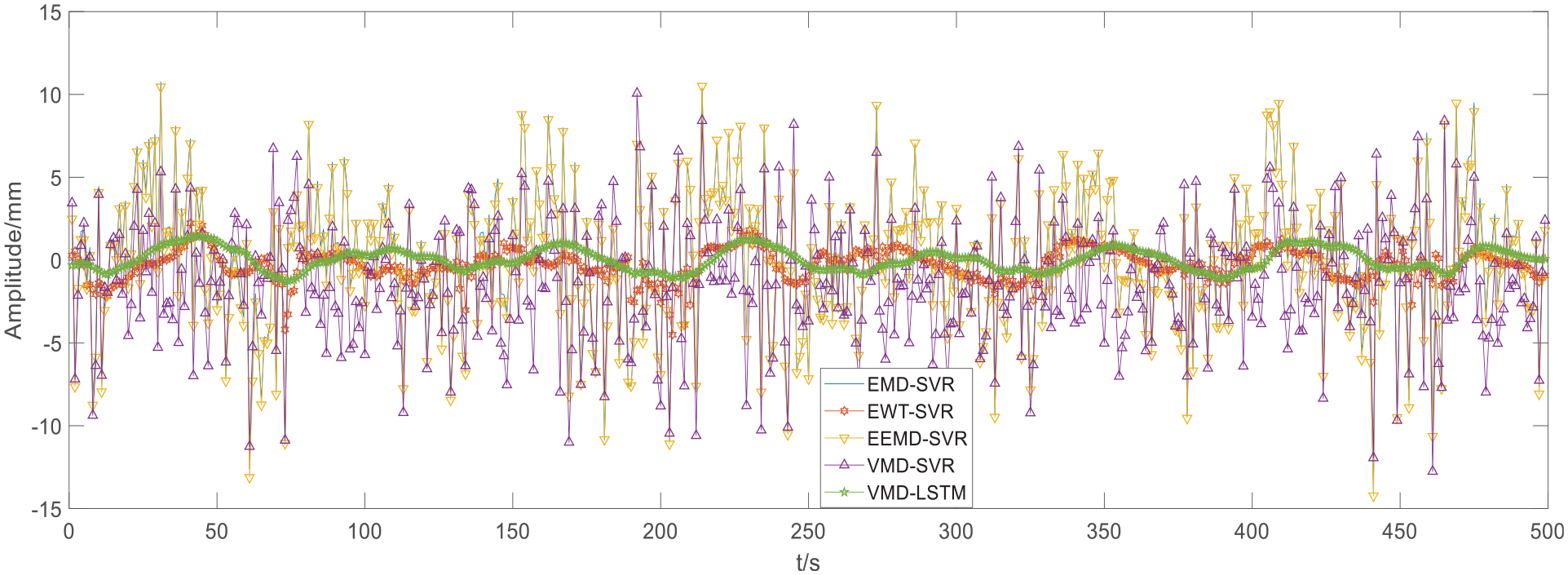
Comparison of the mold-level prediction error of the three methods.

Table 6.

Parameters of the three different methods.

Method	C	g	k
EMD-SVR	16.3485	0.01773	–
EEMD-SVR	16.3485	0.01773	–
EWT-SVR	16.3485	0.01773	–
VMD-SVR	95.5729	0.39511	9
VMD-LSTM			9

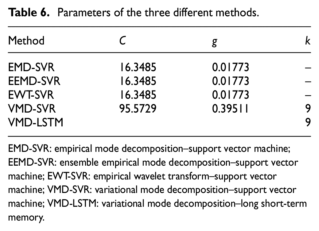
EMD-SVR: empirical mode decomposition–support vector machine; EEMD-SVR: ensemble empirical mode decomposition–support vector machine; EWT-SVR: empirical wavelet transform–support vector machine; VMD-SVR: variational mode decomposition–support vector machine; VMD-LSTM: variational mode decomposition–long short-term memory.

Analysis of prediction results

In this section, the following three statistical indicators are used to verify the performance of the five hybrid prediction algorithms, and the optimal hybrid prediction model suitable for predicting the mold steel level of the mold is selected.

The correlation coefficient is calculated as

R = \frac{Cov (P_{i}, A_{i})}{\sqrt{Var (P_{i}) \cdot Var (A_{i})}}

(16)

The correlation coefficient is used to reflect the statistical relationship between the variables. The larger the correlation coefficient is, the better the performance of the algorithm is.

The formula of root mean square error is

RMSE = \sqrt{\frac{\sum_{i = 1}^{n} {(P_{i} - A_{i})}^{2}}{n}}

(17)

The root mean square error reflects the degree of dispersion of the data set, and the deviation between the observed value and the true value is measured. The smaller the root mean square error is, the better the performance of the algorithm is.

The formula of mean absolute error (MAE) is

MAE = \frac{\sum_{i = 1}^{n} | P_{i} - A_{i} |}{n}

(18)

The average error is the average of the absolute errors, which better reflects the actual situation of the prediction error. The smaller the average error is, the better the performance of the algorithm is.

Here P_i and A_i are the ith predicted mold-level data point and the original mold-level data point, respectively, and n is the total number of predictions.

Table 7 and Figure 11 show the advantages of the VMD-LSTM method from two different perspectives. Table 7 and Figure 11 show that VMD-SVR shows better performance than MMD-SVR because VMD shows better decomposition performance than EMD, and VMD-LSTM shows better performance than VMD-SVR because LSTM shows better prediction performance than SVR. VMD-LSTM’s root mean square error is the smallest, which shows that the model has stronger robustness; its MAE is the largest, reflecting that VMD-LSTM prediction is the most accurate; moreover, mean absolute percentage error (MAPE) considers not only the error between the predicted value and the real value, but also the ratio between the error and the real value, which shows that the VMD-LSTM model has the highest prediction accuracy.

Table 7.

A comparison of the prediction model test results.

	R	RMSE	MAE
EMD-SVR	0.4394	2.0907	3.9493
EEMD-SVR	0.5037	1.2983	3.5725
EWT-SVR	0.8052	0.5368	1.8562
VMD-SVR	0.9988	0.0555	1.1367
VMD-LSTM	0.9998	0.0493	0.9833

RMSE: root mean square error; MAE: mean absolute error; EMD-SVR: empirical mode decomposition–support vector machine; EEMD-SVR: ensemble empirical mode decomposition–support vector machine; EWT-SVR: empirical wavelet transform–support vector machine; VMD-SVR: variational mode decomposition–support vector machine; VMD-LSTM: variational mode decomposition–long short-term memory.

Figure 11.

A comparison of prediction model test results.

It can be seen from Table 7 and Figure 11 that, among the SVR-based hybrid methods, VMD-SVR shows better performance than EMD-SVR. The four indicators are all the best and the prediction performance has been greatly improved. Among the VMD-based hybrid methods, VMD-LSTM shows better performance than VMD-SVR.

The VMD-based hybrid methods show better performance than the SVR-based hybrid methods because VMD has a better data decomposition effect than EMD and empirical wavelet transform (EWT), which can effectively decompose the original signal into different narrow-band signals, thus effectively avoiding the boundary effect of EMD and improving the signal prediction.

Among the VMD-based hybrid methods, the R value of VMD-SVR is close to that of VMD-LSTM. The MAE of VMD-LSTM is 0.9833, which is better than that of VMD-SVR. The performance of VMD-LSTM prediction is better than that of VMD-SVR, LSTM uses an advanced deep neural network framework for calculations, and predictive models exhibit superior predictive performance compared to SVR. The VMD-LSTM hybrid method greatly improves the prediction accuracy compared to the traditional algorithm and shows a strong generalization ability and robustness.

Conclusion

In this article, a novel method for mold-level prediction is proposed. The algorithm combines multiple pattern decomposition algorithms, MIE, and deep learning. It is a prediction algorithm with more adaptive denoising and strong robustness. The algorithm uses a variety of mode decomposition methods to simplify complex mold-level data. The MIE is used to determine the real mode number, the high-frequency IMF threshold, and the low-frequency IMF threshold. In addition, the mold-level data are effectively denoised while saving as much information as possible. Furthermore, the IMF prediction is carried out using a powerful deep learning tool, the LSTM model. Finally, the predicted mold-level data are obtained. The contributions of this article are as follows:

In this article, an MMD-LSTM prediction method is proposed.

In the field of mold-level prediction, the MMD-LSTM prediction algorithm is used for the first time.

By experimenting and comparing the predicted data with the actual signals, the proposed algorithm is shown to be a better prediction algorithm with stronger robustness and powerful generalization ability when compared with the other algorithms.

Although the efficiency and accuracy of the proposed method have been greatly improved, LSTM as a deep learning method consumes a large amount of computational memory. We will improve the cost of the LSTM in the future.

Footnotes

Acknowledgements

Qi Gao, Hang Zhao and Yanni Zheng are acknowledged for their valuable technical support.

Handling Editor: James Baldwin

Author contributions

W.S. conceived and designed the research; Z.L. performed the experiment and wrote the manuscript.

Declaration of conflicting interests

The author(s) declared no potential conflicts of interest with respect to the research, authorship, and/or publication of this article.

Funding

The author(s) disclosed receipt of the following financial support for the research, authorship, and/or publication of this article: This work was financially supported by the National Natural Science Foundation of China (No. 51575429).

ORCID iD

Zhufeng Lei

References

Watanabe

Omura

Konishi

, et al. Mold level control in continuous caster by neural network model. ISIJ Int 1999; 39: 1053–1060.

Lee

Kueon

Lee

. High performance hybrid mold level controller for thin slab caster. Control Eng Pract 2004; 12: 275–281.

Dussud

Galichet

Foulloy

. Application of fuzzy logic control for continuous casting mold level control. IEEE T Contr Syst T 1998; 6: 246–256.

Hesketh

Clements

Williams

. Adaptive mold level control for continuous steel slab casting. Automatica 1993; 29: 851–864.

De Keyser

. Predictive mould level control in a continuous steel casting line. In: Proceedings of the 13th world congress, international federation of automatic control (Vol. M: chemical process control, mineral, mining, metals), San Francisco, CA, 30 June–5 July 1996, pp.487–492. New York: International Federation of Automatic Control.

De Keyser

RMC

. Improved mould-level control in a continuous steel casting line. Control Eng Pract 1997; 5: 231–237.

Kong

De Keyser

Martien

, et al. Model identification for the mould level control loop in a continuous casting machine. In: Proceedings of the 7th IFAC symposium on automation in mining, mineral and metal processing, Beijing, China, 26–28 August 1992, pp.107–112. Amsterdam: Elsevier.

Dekemele

Ionescu

C-M

De Doncker

, et al. Closed loop control of an electromagnetic stirrer in the continuous casting process. In: Proceedings of the 2016 European control conference (ECC), Aalborg, 29 June–1 July 2016, pp.61–66. New York: IEEE.

Copot

Ghita

Ionescu

. Simple alternatives to PID-type control for processes with variable time-delay. Processes 2019; 7: 146.

10.

Huang

Shen

Long

, et al. The empirical mode decomposition and the Hilbert spectrum for nonlinear and non-stationary time series analysis. P Roy Soc A: Math Phy 1998; 454: 903–995.

11.

Lei

Lin

, et al. A review on empirical mode decomposition in fault diagnosis of rotating machinery. Mech Syst Signal Pr 2013; 35: 108–126.

12.

Bajaj

Pachori

. Classification of seizure and nonseizure EEG signals using empirical mode decomposition. IEEE T Inf Technol B 2012; 16: 1135–1142.

13.

Priya

Yadav

Jain

, et al. Efficient method for classification of alcoholic and normal EEG signals using EMD. J Eng 2018; 3: 166–172.

14.

Prasanna Kumar

Kumaraswamy

. Single-channel speech separation using combined EMD and speech-specific information. Int J Speech Technol 2017; 20: 1037–1047.

15.

Guo

Zhao

, et al. Multi-step forecasting for wind speed using a modified EMD-based artificial neural network model. Renew Energ 2012; 37: 241–249.

16.

Tang

Zhao

Yue

, et al. Vibration analysis based on empirical mode decomposition and partial least square. In: Proceedings of the international workshop on automobile, power and energy engineering, vol. 16, Wuhan, China, 15–17 April 2011. Amsterdam: Elsevier.

17.

Tian

Qian

. EMD- and SVM-based temperature drift modeling and compensation for a dynamically tuned gyroscope (DTG). Mech Syst Signal Pr 2007; 21: 3182–3188.

18.

Luo

Yan

Xie

, et al. Hilbert-Huang transform, Hurst and chaotic analysis based flow regime identification methods for an airlift reactor. Chem Eng J 2012; 181: 570–580.

19.

Srinivasan

Rengaswamy

Miller

. A modified empirical mode decomposition (EMD) process for oscillation characterization in control loops. Control Eng Pract 2007; 15: 1135–1148.

20.

Dragomiretskiy

Zosso

. Variational mode decomposition. IEEE T Signal Proces 2014; 62: 531–544.

21.

Zhang

Liu

Qin

, et al. Deterministic and probabilistic interval prediction for short-term wind power generation based on variational mode decomposition and machine learning methods. Energ Convers Manage 2016; 112: 208–219.

22.

Lahmiri

. Comparative study of ECG signal denoising by wavelet thresholding in empirical and variational mode decomposition domains. Healthc Technol Lett 2014; 1: 104–109.

23.

Hochreiter

Schmidhuber

. Long short-term memory. Neural Comput 1997; 9: 1735–1780.

24.

Graves

Beringer

Schmidhuber

. A comparison between spiking and differentiable recurrent neural networks on spoken digit recognition. In: Proceedings of the 23rd IASTED international conference on modelling, identification, and control, 2004.

25.

McCann

Bradbury

Xiong

, et al. Learned in translation: contextualized word vectors. In: Advances in neural information processing systems 30: 31st annual conference on neural information processing systems (NIPS 2017), vol. 30, Long Beach, CA, 4–9 December 2017. Red Hook, NY: Curran Associates, Inc.

26.

Schuster

Chen

, et al. Google’s neural machine translation system: bridging the gap between human and machine translation, 2016, https://arxiv.org/pdf/1609.08144.pdf

27.

Burgsteiner

. Training networks of biological realistic spiking neurons for real-time robot control. In: Proceedings of the 9th international conference on engineering applications of neural networks, Lille, France, 2005, pp.129–136.

28.

Peng

Andrychowicz

Zaremba

, et al. Sim-to-real transfer of robotic control with dynamics randomization. In: Proceedings of the IEEE international conference on robotics and automation (ICRA), 21–25 May 2018; Brisbane, QLD, Australia, pp.3803–3810. New York: IEEE.

29.

Byeon

Liwicki

Breuel

. Texture classification using 2D LSTM networks. In: Proceedings of the 22nd international conference on pattern recognition (ICPR), Stockholm, 24–28 August 2014, pp.1144–1149. New York: IEEE.

30.

Malinowski

Rohrbach

Fritz

. Ask your neurons: a neural-based approach to answering questions about image. In: Proceedings of the IEEE international conference on computer vision, 11–18 December 2015, Santiago, Chile, pp.1–9. New York: IEEE.

Mold-level prediction based on long short-term memory model and multi-mode decomposition with mutual information entropy

Abstract

Keywords

Introduction

Basic algorithms

The basic principle of VMD

The basic principle of LSTM

MIE

Mold-liquid-level prediction based on MMD-LSTM

Test analysis

Data source

MMD-LSTM-based mold-liquid-level prediction

Analysis of prediction results

Conclusion

Footnotes

Acknowledgements

Author contributions

Declaration of conflicting interests

Funding

ORCID iD

References