Sage Journals: Discover world-class research

Abstract

In order to estimate the light-duty vehicle fuel economy at high-altitude areas, the coast-down tests of a passenger car on level road were conducted at different elevations, and the coast-down resistance coefficients were calculated. Furthermore, a fuel economy model for a light-duty vehicle adopting backward simulation method was developed, and it mainly consists of vehicle dynamic model, internal combustion engine model, transmission model, and differential model. The internal combustion engine model consists of the brake-specific fuel consumption maps as functions of engine torque and engine speed, and the brake-specific fuel consumption map near sea level was constructed based on engine experimental data, and the brake-specific fuel consumption maps at high altitudes were calculated by GT-Power Modeling of the internal combustion engine. The fuel consumption rate was calculated from the brake-specific fuel consumption maps and brake power and used to calculate the fuel economy of the light-duty vehicle. The model predicted fuel consumption data met well with the test results, and the model prediction errors are within 5%.

Keywords

Light-duty vehicle fuel economy coast-down test model prediction high altitude

Introduction

Vehicle fuel economy and emissions are influenced by many parameters, including vehicle-related factors such as model, make, mass, size, fuel type, technology level, and mileage,¹ and operating factors such as speed, acceleration, deceleration, gear shift, road gradient, and ambient conditions including headwind, ambient pressure and temperature, and so on.² Among the ambient conditions, the altitude has significant influence on the vehicle fuel consumption and emissions, and it is crucial to clarify that there are significant discrepancies between the type approval test conditions and high-altitude driving conditions.

Plenty of studies investigate the diesel engine performance under high-altitude conditions using an atmosphere simulating device, which varies the intake and exhaust pressures in order to simulate the high-altitude environment. Compared to vehicles operation at sea level, diesel engines running under high-altitude conditions produce more CO, HC, and PM emissions^3,4 and increased smoke opacity.⁵ As for NOx, it was insensible to the variation of altitude in some studies. Due to the decrease in the air pressure and oxygen density with the increasing altitudes, the diesel engine combustion deteriorates and results in decreased thermal efficiency, reduced power output, and increased fuel consumption,^6–10 especially in comparison with the engine operation at near sea level.

Zervas¹¹ studies the impact of high altitude on the fuel consumption of a gasoline passenger car. The tests were performed using an altimetric test bench located at an altitude of 70 m by decreasing atmospheric pressure to simulate high altitude. The fuel consumption of a Renault Clio car equipped with a Euro 3 gasoline engine were tested at the altitude of 70 and 2200 m. He studied the impact of high altitude on the fuel consumption of the gasoline passenger car over three regulated driving cycles and concluded that the impact of higher altitude is not evident. This conclusion was drawn based on the experimental results at two altitudes of 70 and 2200 m. More work need to be done to clarify the impact of higher altitude on vehicle fuel consumption.

In recent years, on-vehicle emission measurement systems are widely used. Wang et al.¹² studied the effects of altitude on the thermal efficiency and emission characteristics of a Euro 3 diesel engine using a mobile engine test bench and a portable emission measurement system (PEMS), and found that the engine thermal efficiency decreased and the emission of CO, HC, and particulate matter (PM) increased with altitude. Ramos et al.¹³ studied the effect of altitude on emissions from a light-duty vehicle under real-world driving conditions and found that NOx emissions increased with altitude.

Although the engine performance will deteriorate at high-altitude areas, the vehicle driving resistance will also decrease due to decreased air pressure and density with the increase in the altitude. The comprehensive effects of these two factors on the vehicle fuel consumption characteristics need to be further investigated. And, the road load resistance of the light-duty vehicle on a real driving road must be accurately measured.

In fact, the engine performances of new passenger cars are usually tuned and calibrated at the sea level. However, plenty of vehicles are used at high-altitude areas rather than near the sea level, for example, in China, nearly 65% of total territories are high-altitude regions over 1000 m above sea level and 33% of area are 2000 m higher than sea level. The total registered population of vehicles in some high-altitude provinces including Yunnan, Qinghai, and Tibet accounts for 20% of the total number of vehicles in China.¹⁴ Therefore, it is very important to investigate the impact of altitude on vehicle fuel consumption and emissions. However, few studies were conducted on the vehicle driving resistance and fuel consumption by experiment at high-altitude regions.

In this article, the coast-down tests of a passenger car on the actual road were conducted at different altitudes, and the road resistance and fuel consumption of the vehicle were measured. Based on the experimental results, a vehicle fuel economy model was developed to simulate the vehicle fuel consumption at different altitudes, and validated by the experimental results.

Experimental section

In the automotive industry, the vehicle driving resistance is usually tested and confirmed by the coast-down test, which fulfills the measurement of vehicle road load on a dry, straight, level road at speeds less than 130 km/h. The SAE Recommended Practices^15,16 provide the uniform testing procedures for measuring the road load force on a vehicle as a function of vehicle velocity. In this article, the coast-down tests of a passenger car on the actual road were conducted at different altitudes, the coast-down tests were performed in both directions and repeated many times to reduce tolerances which were caused by road gradient and effects of wind direction.

In practice, the total coast-down resistance of the vehicle on real road is generally expressed as a second-order fit that includes a term that is linear in vehicle speed

F_{res} = f_{0} + f_{1} v + f_{2} v^{2}

(1)

where $F_{res}$ is the coast-down resistance force; $f_{0}$ , $f_{1}$ , and $f_{2}$ are the on-road coast-down coefficients. In theory, $f_{1}$ should be zero, but in practice, it is more often non-zero due to the characteristics of the tires.

Test vehicle

The test vehicle was a passenger car made by Volkswagen Company. Its mechanical specifications are given in Table 1.

Table 1.

Test vehicle specifications.

Vehicle	Passenger car
Model year	2012
Make	Volkswagen
Engine	1.4 T
Fuel	Gasoline
Size (length × width × height)	4.87 m × 1.834 m × 1.472 m
Transmission	Manual, 5 speed
Weight	1435 kg
Tire dimensions	215/60 R16
Rated power	96 kW (5000 r/min)
Maximum torque	220 N m (1750–3500 r/min)

Testing equipments

Testing equipments used in the vehicle coast-down tests are listed in Table 2.

Table 2.

Testing equipments.

Equipment	Model	Measurement range	Accuracy
GPS navigator	Oregon 550	Barometric pressure: 100–1100 hPa; Altitude: −200 to 10,000 m	Barometric pressure: ± 0.3 hPa; Altitude: 5 m
Non-contact speed meter and fuel flow meter	Flowtronic 206/207/4705	Vehicle speed: 0–250 km/h Fuel flow rate: 0–60 L/h	Vehicle speed: ±0.5% Fuel flow rate: ±0.5%
Automatic weather station	PH-1	Wind speed: 0–45 m/s Wind direction: 0°–360° Atmospheric temperature: −50°C to 100°C Atmospheric moisture: 0%–100% RH; Barometric pressure: 10–1100 hPa	Wind speed: ±0.3 m/s; Wind direction: ±3°; Atmospheric temperature: ±0.2°C; Atmospheric moisture: ±3% RH; Barometric pressure: ±0.3 hPa;
Barometric pressure monitor	TRM-QA	Barometric pressure: 450–1100 hPa; Atmospheric temperature: −50°C to 100°C; Altitude: −500 to 9000 m	Barometric pressure: ±0.3 hPa; Atmospheric temperature: ±0.2°C; Altitude: 5 m
Tire pressure monitoring system	Schrader	Temperature: −40°C to 60°C; Tire pressure: 0–10 bar

The Oregon 550 GPS receiver receives the vehicle geographical location information from satellites and performs the necessary calculations to determine the vehicle current position, speed, and heading. These data are used to calculate the altitude, vehicle speed, and road gradient.

Flowtronic 206-207 is an automatic road testing instruments made by Switzerland QUICKLY AG Company. In this research, Flowtronic 206-207 was used to measure and record vehicle speed and acceleration. And, the Flowtronic 4705 high-resolution fuel flow meter was used for the vehicle’s fuel consumption testing.

The PH-1 automatic weather station is used to measure the relative wind speed and wind direction relative to the direction of vehicle travel, and also used to measure the atmospheric temperature, humidity, and barometric pressure.

The TRM-QA barometric pressure monitor is utilized to measure the barometric pressure, atmospheric temperature, and altitude. By calculating the derivative of altitude with respect to the distance traveled, the road gradient could be calculated.

The Schrader tire pressure monitoring system is used to monitor the tire Pressure and temperature.

Coast-down test

The goal of coast-down test is to determine the road load force of a passenger car at different altitudes.

The testing was performed on long flat and straight asphalt roads at different altitudes. It was important to perform the testing in both directions in order to eliminate the effects of the grade and wind. Based on SAE Standards J1263¹⁵ and J2263,¹⁶ the test vehicle was fully warmed before each test, and the measurement instruments were also pre-warmed and calibrated before testing.

The ambient temperature and altitude of each test sites are recorded and listed in Table 3.

Table 3.

Ambient conditions of the test sites.

No.	Altitude (m)	Average temperature (°C)
1	21	25
2	842	23.6
3	1520	21.2
4	2676	16.2
5	3030	15.8

For each testing, the car was speeded up to 130 km/h on the test track and then testing was conducted with the transmission in neutral. Knowing the vehicle direction, wind speed, and wind direction, wind-related aerodynamic drag forces can be filtered out of the raw deceleration data.

The vehicle coast-down resistances were calculated using a numerical method of linear least square regression to calculate the constants in function 1. As shown in Figure 1, the x-axis is on the square scale. The intercept of the line represents the rolling resistance, and the slope stands for the aerodynamic drag coefficient. Based on the regression functions, the constants of five regression functions are nearly equal and show that the rolling resistance is almost not influenced by altitude, while the different slopes show that the aerodynamic drag force is evidently influenced by altitude due to the variation of air pressure and density with the elevation.

Figure 1.

Fitted linear regression of coast-down resistance under different altitudes.

Vehicle fuel economy model

The air pressure and density decrease at high-altitude areas, and will significantly influence the vehicle driving resistance and the engine performance. It was very difficult in performing experiments to test vehicle driving resistance at high-altitude areas, because it was hard to find a level road long enough to carry out the vehicle coast-down test, and the experiment was complicated, expensive, and time-consuming. The complicated characteristics of vehicle performance and the diversity of driving conditions also make it necessary to utilize simulation models to predict or evaluate the vehicle performances, especially for vehicle at high-altitude areas. Based on the experimental results obtained at high-altitude regions, a vehicle fuel economy model was developed to simulate and predict the vehicle fuel economy performance.

Vehicle fuel economy model

The vehicle fuel economy model, as shown in Figure 2, consists of a vehicle dynamic model, an internal combustion (IC) engine model, a transmission model, a differential model, and driven wheels. The torque and rotating speed from the output shaft of the engine are transmitted to the driven wheels through the gearbox, differential, and drive shaft. The gearbox supplies certain gear ratio from its input shaft to its output shaft for the engine torque speed profile to match the requirements of the load. The final drive is a pair of gears that provide a further speed reduction and distribute the torque to each wheel through the differential.

Figure 2.

Vehicle fuel economy model.

In this research, the inputs to the vehicle fuel economy model are the driving cycle, vehicle coast-down coefficients, vehicle weight, and so on. Some of the model inputs are implicit in the model in order that the user does not have to input them directly. The outputs of the vehicle fuel economy model are vehicle dynamic performance and economic performance.

The motive torque acting on the drive axles can be calculated by multiplying the motive force and drive tire rolling radius. By calling the transmission model and the differential model, the transmission input torque and revolution speed, which are required from the engine output torque and engine revolution speed, can be calculated. Finally, the vehicle dynamic model would call the engine model to calculate the fuel consumption at that second of the driving cycle and calculate the vehicle fuel consumption over the selected driving cycle.

The transmission model includes the gear shift strategy, which determines shift pattern depending on speed and load. The transmission model considers various types of transmissions, including manual and automatic. The gear shift strategy is executed, and the gear ratio will be determined by the transmission input speed and load. The transmission model and the differential model will also calculate power transmission efficiency for each gear ratio.

The IC engine model consists of the brake-specific fuel consumption (BSFC) maps as functions of the engine torque and revolution speed. The BSFC map near sea level was constructed based on engine experimental data, and the BSFC maps at high altitudes were calculated by GT-Power Modeling of the IC engine.

IC engine model

In order to obtain the engine BSFC maps at high altitudes, a GT-Power engine model was established based on the 1.4-T gasoline engine specifications,¹⁷ calibrated and validated by the engine experimental data near sea level. As shown in Figure 3, the GT-Power engine model composed of the intake and exhaust model, intercooler and supercharging model, cylinder and combustion model, post-processing model, and so on, was used to predict engine performances including power, torque, and fuel consumption. The BSFC maps under high-altitude conditions were calculated by GT-Power engine model by setting the ambient atmospheric conditions.

Figure 3.

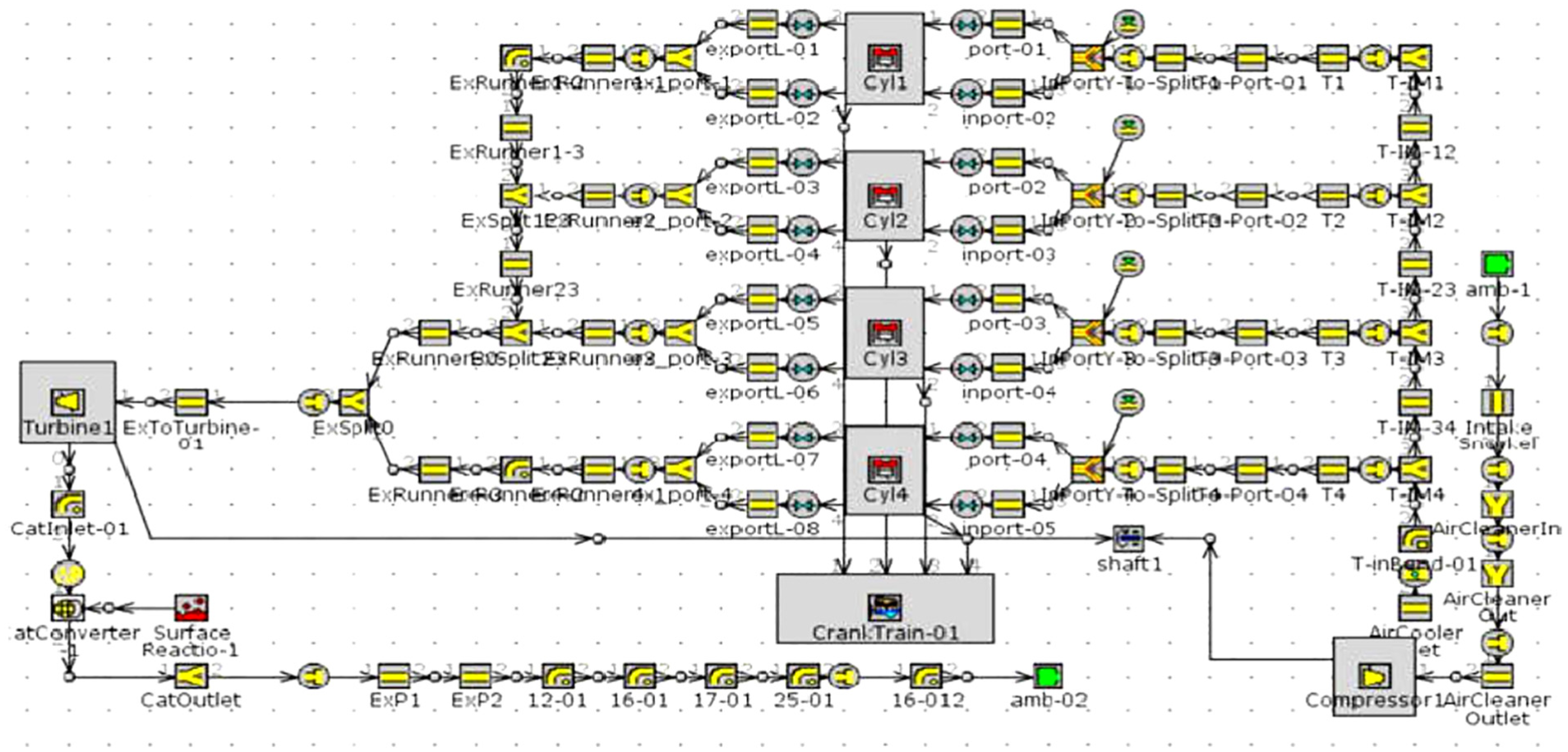
GT-Power engine model.

Figure 4 shows the dynamic and fuel economy performances of the 1.4-T gasoline engine operating with wide open throttle position at different altitudes. As shown in Figure 4(a), the maximum torques of the engine over the whole speed range decrease with the increase in the altitude. And, as depicted in Figure 4(b), with the increase in the power output, the engine fuel economy performances deteriorate with the increase in the altitude.

Figure 4.

Engine performances at wide open throttle position: (a) engine dynamic performance and (b) engine fuel economic performance.

By utilizing the GT-Power engine model of the 1.4-T gasoline engine, the engine fuel consumption maps at different altitudes were calculated, and showed in Figure 5.

Figure 5.

Engine BSFC maps at different altitudes: (a) at the altitude of 21 m, (b) at the altitude of 1000 m, (c) at the altitude of 2000 m, (d) at the altitude of 3000 m, and (e) at the altitude of 4000 m.

By comparing the engine fuel consumption maps over the whole engine operation areas at different altitudes, we can see that the engine maximum torque decreases significantly with the increase in the altitude. In the meantime, with the increase in the altitude, the engine fuel economy performance deteriorates, and the area of engine low-fuel-consumption regions decreases with the increase in the altitude.

All the engine fuel consumption maps at different altitudes were all embedded into the IC engine model and used for calculating vehicle fuel consumption.

Vehicle performance simulation method

There are two different methods to predict the fuel consumption over the selected driving cycle: “forward simulation approach” and “backward simulation approach.”^18,19 In this article, the backward simulation approach was adopted, as shown in Figure 2, the vehicle fuel economy model does not require a driver model. The backward simulation approach assumes that the vehicle speed can exactly match the selected driving cycle, so that the engine revolution speed can be directly calculated using vehicle speed, the tire rolling radius, the transmission gear ratio, and the differential gear ratio, and expressed as

n_{e} = \frac{i_{g} i_{0} V}{2 π R_{w}}

(2)

where $n_{e}$ is the engine revolution speed, $i_{g}$ is the transmission gear ratio, $i_{0}$ is the differential gear ratio, $V$ is the instantaneous vehicle speed, and $R_{w}$ is the tire rolling radius.

The motive force required to accelerate the vehicle is also calculated directly based on the vehicle speed sequence derived from the driving cycle. The required motive force is then transformed into a required torque by multiplying the motive force and drive tire rolling radius. The coast-down coefficients measured through coast-down test were used to calculate the vehicle road resistance at different altitudes.

When the vehicle drives on level road when the wind is negligible, the required engine torque can be calculated by

T_{e} = \frac{((1 + ε) m \frac{dV}{dt} + f_{0} + f_{1} V + f_{2} V^{2}) R_{w}}{i_{g} i_{0} η_{t}}

(3)

where $T_{e}$ is the required engine torque; $m$ is vehicle mass; $ε$ is “mass factor,” which is the equivalent ratio of translational mass of the rotating components (wheels, gears, shafts, etc.) of the powertrain; $f_{0}$ , $f_{1}$ , and $f_{2}$ are the coast-down coefficients; and $η_{t}$ is the efficiency of the driveline from the engine to the driven wheels.

During the simulation, the fuel consumption rate is calculated through the engine power and BSFC maps, and will be accumulated for the whole driving cycle. And then, the total amount of fuel consumption will be divided by the vehicle traveled distance to calculate the vehicle fuel consumption per 100 km travel distance.

In the vehicle fuel economy model, the vehicle dynamic model used altitude, engine revolution speed, and engine torque as key parameters to interpolate the engine BSFC maps to calculate the instant fuel consumption rate. Second by second, fuel consumption rate results are accumulated to calculate the total fuel consumption during the whole driving cycle

Q_{tot} = \sum \frac{k \cdot T_{e} \cdot n_{e} \cdot b_{e}}{D} \cdot Δ t

(4)

where $Q_{tot}$ is the total fuel consumption volume in Liter, $k$ is a constant, $b_{e}$ is the instant fuel consumption rate in g/kWh at time $t$ , $Δ t$ is the simulation time step, and $D$ is the density of the gasoline fuel.

In the same way, we calculate the vehicle total travel distance by

S_{tot} = \sum^{V_{t}} \cdot Δ t

(5)

where $S_{tot}$ is the accumulated vehicle travel distance in km, $V_{t}$ is the vehicle speed at time $t$ , and $Δ t$ is the simulation time step.

As a result, we can calculate the vehicle fuel consumption per 100 km travel distance by

Q_{s} = \frac{Q_{tot}}{100 \cdot S_{tot}}

(6)

The vehicle fuel economy simulation program was written in MATLAB. If a second-by-second velocity profile is defined, the instantaneous fuel consumption can be calculated. And, if the average vehicle driving characteristics such as average speed are given, this vehicle fuel economy model can also estimate vehicle fuel economy based on the average vehicle activity parameters. Therefore, the vehicle fuel economy model can be implemented into micro-simulation intelligent transport system (ITS) applications.

Model validation

The vehicle fuel economy model was validated by the vehicle real road fuel consumption test results measured at different altitude areas. The driving cycle used for model validation was chosen from the experimental data collected from the real road driving experiments.

At the previous mentioned four high-altitude places, the vehicle fuel consumption tests were performed at the speed of 50, 60, 80, 90, 100, and 120 km/h respectively, and compared with the vehicle model predicted fuel consumption data at the same speed. The reason why we tested the constant speed vehicle fuel consumption and compared with the predicted ones is to validate and evaluate the vehicle fuel economy model prediction capability at high altitudes and alleviate the affects of other factors.

It is necessary to warm the test vehicle to a hot stabilized state before test. In this research, the test vehicle was driven at a speed greater than 75 km/h for at least 30 min. And, the warming procedure was the same for all the tests.

The Flowtronic 206/207/4705 fuel flow meter was used to measure and record vehicle speed and fuel consumption data. The vehicle fuel consumption test was performed at least three times for each speed to ensure a fuel consumption difference of less than 2% in the three repetitions.

The tested fuel consumption data were compared with the model predicted fuel consumption results, as shown in Table 4, and Figure 6(a)–(d) shows the comparison of the model predicted fuel consumption and the tested raw data at the altitude of 842, 1520, 2676, and 3030 m, respectively. The results showed that vehicle fuel consumption per 100 km increases with vehicle speed due to the increased driving resistances, no matter how high the altitude of the test sites is. The model predicted fuel consumption data met well with the test results, and the model prediction errors are within 5%.

Table 4.

Comparison of predicted fuel consumption data and the tested raw data.

Altitude (m)	Speed (km/h)	Tested data (L/100 km)	Predicted data (L/100 km)	Error (%)
842	50	4.37	4.53	3.66
	60	5.41	5.52	2.03
	80	7.64	7.74	1.31
	90	9.85	9.98	1.32
	100	10.68	10.87	1.78
	120	11.64	11.96	2.75
1520	50	5.12	5.01	−2.05
	60	5.58	5.49	−1.57
	80	6.56	6.67	1.68
	90	7.63	7.61	−0.26
	100	8.56	8.72	1.87
	120	9.41	9.57	1.70
2676	50	4.69	4.75	1.28
	60	5.74	5.79	0.87
	80	6.56	6.71	2.29
	90	6.95	7.03	1.15
	100	7.74	7.89	1.94
	120	8.89	8.99	1.12
3030	50	6.3	6.39	1.50
	60	7.42	7.34	−1.02
	80	8.44	8.42	−0.28
	90	9.64	9.74	1.05
	100	10.38	10.48	0.98
	120	12.74	12.98	1.90

Figure 6.

Vehicle fuel consumption per 100 km as a function of vehicle speed: (a) at the altitude of 842 m, (b) at the altitude of 1520 m, (c) at the altitude of 2676 m, and (d) at the altitude of 3030 m.

Figure 7(a)–(f) showed the predicted fuel consumption data and the tested raw data as a function of the altitude under different vehicle speeds.

Figure 7.

Vehicle fuel consumption per 100 km as a function of altitude under different vehicle speeds: (a) under the speed of 50 km/h at fourth gear, (b) under the speed of 60 km/h at fourth gear, (c) under the speed of 80 km/h at fifth gear, (d) under the speed of 90 km/h at fifth gear, (e) under the speed of 100 km/h at fifth gear, and (f) under the speed of 120 km/h at fifth gear.

Figure 7 showed that at vehicle speed lower than 80 km/h, the vehicle fuel consumption at high altitude does not change significantly due to the cooperative effect of the degraded engine fuel economy and decreased driving resistance with the increase in the altitude. But when vehicle speed is higher than 80 km/h, the rapid decreased driving resistance plays a dominant role and the engine load decreased and totally compensates the degraded engine fuel economy, leading to decreased vehicle fuel consumption until the altitude of 2800 m. When the altitude is higher than 2800 m, the engine combustion and fuel economic performance become worse significantly and that leads to increased vehicle fuel consumption despite decreased driving resistance.

Conclusion

In this article, the coast-down tests for a light-duty gasoline vehicle were carried out at different altitudes, and the road load coefficients of the gasoline vehicle were calculated. The vehicle on-road resistive force at high altitude decreases due to the decreased air density and resistance, especially at high vehicle speed.

A light-duty vehicle fuel economy model adopting backward simulation method was developed, and it mainly consists of vehicle dynamic model, IC engine model, transmission model, and differential model. The IC engine model consists of BSFC maps as functions of the engine torque and engine speed, and the BSFC maps at different altitudes were calculated by GT-Power Modeling of the gasoline engine. The fuel consumption rate was calculated from the BSFC maps and brake power and used to calculate the vehicle fuel economy. The model predicted fuel consumption data met well with the test results, and the model prediction errors are within 5%.

Footnotes

Handling Editor: James Baldwin

Declaration of conflicting interests

The author(s) declared no potential conflicts of interest with respect to the research, authorship, and/or publication of this article.

Funding

The author(s) disclosed receipt of the following financial support for the research, authorship, and/or publication of this article: This work was supported by the National Natural Science Foundation of China (No. 51576016) and National Key R&D Plan (No. 2017YFF0211802).

ORCID iD

Lijun Hao

References

Zhang

Liu

, et al. Real-world fuel consumption and CO₂ (carbon dioxide) emissions by driving conditions for light-duty passenger vehicles in China. Energy 2014; 69: 247–257.

Palencia

JCG

Sakamaki

Araki

, et al. Impact of powertrain electrification, vehicle size reduction and lightweight materials substitution on energy use, CO₂ emissions and cost of a passenger light-duty vehicle fleet. Energy 2015; 93: 1489–1504.

Dennis

JW.

Turbocharged diesel engine performance at altitude. SAE technical paper 710822, 1971.

Human

Ullman

Baines

TM.

Simulation of high altitude effects on heavy-duty diesel emissions. SAE technical paper 900883, 1990.

Chemich

Jacobs

Kowalski

JD.

A comparison of heavy duty diesel truck engine smoke opacities at high altitude and at sea level. SAE technical paper 911671, 1991.

Benjumea

Agudelo

Effect of altitude and palm oil biodiesel fuelling on the performance and combustion characteristics of a HSDI diesel engine. Fuel 2009; 88: 725–731.

, et al. Emission characteristics of a heavy-duty diesel engine at simulated high altitudes. Sci Total Environ 2011; 409: 3138–3143.

Shen

Yan

, et al. Combustion process of diesel engines at regions with different altitude. SAE technical paper 950857, 1995.

Liu

Shen

, et al. Effects of altitude and fuel oxygen content on the performance of a high pressure common rail diesel engine. Fuel 2014; 118: 243–249.

10.

Perez

Boehman

AL.

Performance of a single-cylinder diesel engine using oxygen-enriched intake air at simulated high-altitude conditions. Aerosp Sci Technol 2010; 14: 83–94.

11.

Zervas

Impact of altitude on fuel consumption of a gasoline passenger car. Fuel 2011; 90: 2340–2342.

12.

Wang

Yin

, et al. On-vehicle emission measurement of a light-duty diesel van at various speeds at high altitude. Atmos Environ 2013; 81: 263–269.

13.

Ramos

Garcia-Contreras

Armas

Performance, combustion timing and emissions from a light duty vehicle at different altitudes fueled with animal fat biodiesel, GTL and diesel fuels. Appl Energ 2016; 182: 507–517.

14.

Ministry of Environmental Protection (MEP) of China. China vehicle emission control annual Report. Beijing, China: MEP, 2017 (in Chinese).

15.

SAE J1263:2009. Road load measurement and dynamometer simulation using coastdown techniques (revised).

16.

SAE J2263:2008. Road load measurement using onboard anemometry and coastdown techniques (revised).

17.

Emission and performance simulation of turbocharged gasoline engine at high altitude areas. Beijing Institute of Technology, 2016 (in Chinese).

18.

Montazeri-Gh

Varasteh

Naghizadeh

. Driving cycle simulation for heady duty engine emission evaluation and testing. SAE technical paper 2005-01-3796, 2005.

19.

Wipke

Cuddy

Burch

SD.

ADVISOR 2.1: a user-friendly advanced powertrain simulation using a combined backward/forward approach. IEEE T Veh Technol 1999; 48: 1751–1761.

Model-based estimation of light-duty vehicle fuel economy at high altitude

Abstract

Keywords

Introduction

Experimental section

Test vehicle

Testing equipments

Coast-down test

Vehicle fuel economy model

Vehicle fuel economy model

IC engine model

Vehicle performance simulation method

Model validation

Conclusion

Footnotes

Declaration of conflicting interests

Funding

ORCID iD

References