
Abstract
Two axisymmetric dimensional Eulerian/Eulerian simulation of two-phase (gas/liquid) transient flow was performed for both stationary and rotating columns under zero gravity. Multiphase flow simulation is modelled using flow algorithm based on the finite-volume method to simulate bubble population balance modelling. Two coalescence kernels, one for laminar flow and the other for laminar shear flow, are experimented under zero gravity using special user defined functions. Effects of rotation speed are investigated at angular velocities of 0, 0.25, 0.5, 0.75 and 1 rad/s, and effects of air inlet velocity are conducted at 1, 2, 3 and 4 cm/s. The numerical results show that the centrifugal force is pulling the bubbles towards the axis of rotation and shifts them away from the wall. Also, rotation could accelerate the moving bubbles throughout the column under zero-gravity conditions. Increasing the inlet air velocity accelerates the coalescence rate with a decrease in the inlet bubble diameter. Under zero gravity, the bubbles are formed with limited size distribution and may not be represented by an equivalent phase with Sauter mean diameter. Coalescence and break-up phenomena must be considered under normal gravity and coalescence phenomenon only under zero gravity.
Keywords
Introduction
The size distribution of the bubbles plays a critical role in mass transfer and reactions that may occur between any two phases. Detailed knowledge about the bubble–bubble interaction is of great importance for improving bubble contact and increasing efficiency of the bubble column. 1 The bubble–bubble interaction in bubble column reactors is affected by different operating parameters such as initial boundary conditions of the two phases (gas and liquid) as well as outside forces such as column rotation, vibration and pulsation. Hence, resolving the bubble size distribution is an important task in the analysis of bubble column reactors. Also, it is of great importance to model these phenomena in order to manage the dynamics of the bubble formation and enhance the performance of column reactors.
Population balance is a statistical model that is used for the coalescence and break-up of an immiscible fluid. It is one of the most frequently used modelling tools to investigate the large size distribution of the dispersed gas bubble and accounting for the break-up and coalescence effects in bubble column flows. The application of population balance technique started in 1984 and widely spread over the years. 2 Those authors stated over 30 review papers on the topic, between years 1979 and 2013, a variety of application fields. This reflects the wide range of applications of population balances technique to particulate systems, mainly in engineering. Additional review articles of the topic emerged in the recent years by a number of authors.3–7 Sarhan et al. 8 published a number of recent papers on computational fluid dynamics (CFD) modelling of population balance equation in various applications such as flotation cells and flotation columns.9–11 The authors also studied the effect of particle attachment and detachment 12 and the effect of particle size and concentration on bubble coalescence. 11 The population balance technique is also used for fluidized bed 13 and subcooled boiling. 14 It should be stated here that similar techniques to the population balance technique were reported.15,16 The discrete method was developed by Hounslow and colleagues17,18 and Ramkrishna. 19 It is based on representing the continuous particle size distribution (PSD) in terms of a set of discrete size classes or bins.
Swirling flows appear in spray drying towers, burners, cyclone separators and a wide variety of other process systems and are among the most common and most complex in the process industry. “Water droplets in petroleum lines and vapour bubbles in cryogenic fluids in microgravity conditions are some other applications in which the two phases need to be separated from the mixture.” 20 Despite the stated extensive literature on population balances technique for the bubble columns under normal gravity, little work was reported under microgravity environment;21,22 this work is related to medical field not to bubble columns. Previous studies have shown that there is much still to be understood about thermocapillary flow and interaction of bubbles, 23 and there is a lack of information available on the interaction of a group of bubbles/droplets.
However, under zero gravity, coalescence undergoing rotational force holds the key to control the bubble aggregation as seen in the earlier work reported.24,25 To date, the understanding of the low-gravity bubbles coalescence behaviour is limited mainly due to the unresolved physical mechanisms that lead to coalescence and the lack of information because of the difficulties in obtaining the experimental result in microgravity, especially for a rotating column. Up to the best of the authors’ knowledge, there has been no simulation study investigating bubble size distribution under both rotation and zero-gravity condition. In addition, collection kernels used for the population balance modelling are complex and have not yet been benchmarked for zero-gravity environments. Thus, the work reported in this article fills this gap of knowledge.
In the present work, bubble population balance equation (BPBE) in the Euler–Euler CFD representation is used to assess the effect of inlet gas velocity on the bubble collision and agglomeration in microgravity environment. The implemented population balance models (PBMs) will also be used to perform two-dimensional (2D) axisymmetric simulation of air bubbles flow in a rotational column to investigate the possibility of using a rotating cylinder for bubble population modelling under zero gravity. First, the implemented PBMs in a CFD Eulerian–Eulerian model of air-water bubble column flows will be validated with the experimental data of Degaleesan et al., 26 and the population balance simulations performed by Chen et al. 27 under normal gravity. The validated PBM code will also be subjected to grid dependency checks. Then, the investigation of air bubbles flow under zero gravity will be carried out based on the details of the bubble–bubble interaction for rotating cylinders given in the earlier works of Alhenda and colleagues.23,28,29 In this study, a purely coalescing mechanism for bubble growth will be considered and the extent to which coalescence occurs is discussed. A rotating bubble column with varying rotational speed of 0, 0.25, 0.5, 0.75 and 1 rad/s about its axis of symmetry is considered. In addition, the effect of air inlet velocity is investigated at various values of 1, 2, 3 and 4 cm/s.
Numerical methodology
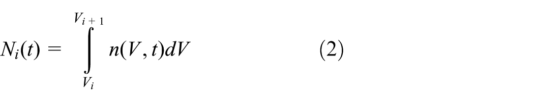
In the current solver, population balance modelling equations (PBME) are written in terms of volume fraction of bubble size i 30

where

where
and

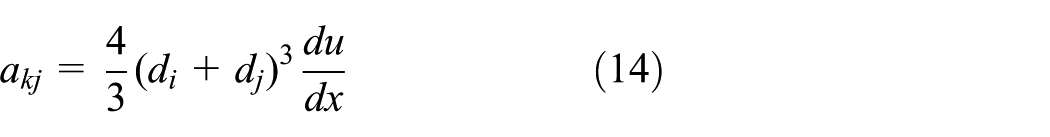
where

The volume coordinate is discretized as


here

where

If

Note that, in general, there is no breakage for the smallest bubble class. 30 For more details on the FLUENT PBM and its application in solving multiphase flows involving a secondary phase with a size distribution, the readers are encouraged to refer to the PBM Manual. 31
Computational settings and validation of the PBM model
The first part of this work is to combine a coalescence and break-up model with a complete flow numerical simulation under normal gravity. The flow equations are solved using a population balance approach coupled with the Eulerian multiphase model. The population balance module is provided as an add-on with the standard FLUENT solver. A two-phase air–water bubble column with a height of 200 cm and diameter of 14.5 cm is used for the simulation. The geometry and operating conditions are all based on the air–water experimental system of Degaleesan et al., 26 which have been validated by simulation from Chen et al. 27 and Law and Battaglia 32 The initial diameter of the injected air bubbles is 0.4 cm as specified by Degaleesan et al. 26 In accordance with Hounslow et al., 17 prescribed bubble classes are chosen in such a way that the bubble volume (or mass) in class i + 1 is twice the volume (or mass) of the antecedent class below i

where i refers to the bubbles size group and n = 2, that is, classes were assigned such that the volume of classi+1 is twice the volume of the antecedent class i (vi + 1 = 2vi). For the purpose of PBM validation, six bubble sizes from 0.159 to 1.62 cm diameter are considered as shown in Table 1, and bubble size of only the third class, that is, 0.4 cm enters the column; these settings are consistent with those of Degaleesan et al. 26
Assigned bubble sizes of n = 2 for the population balance simulation.

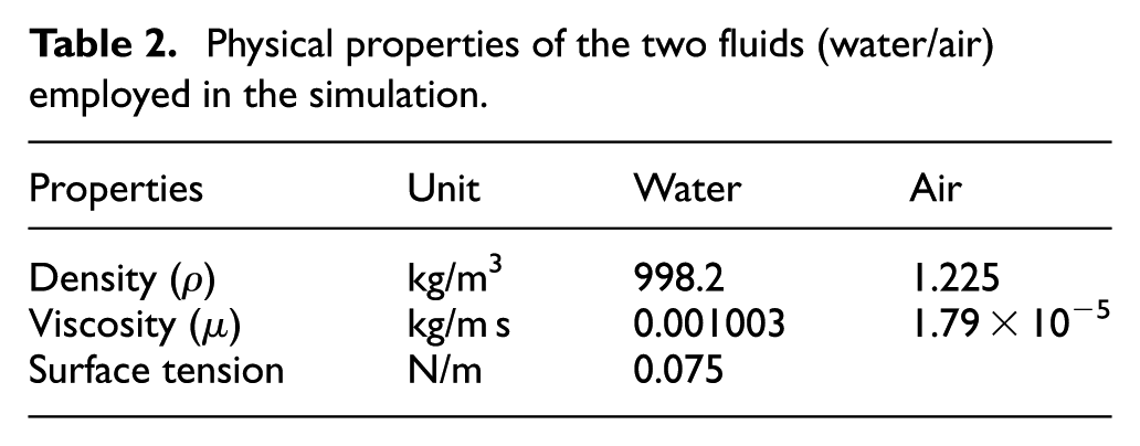
The properties for air and water used in the simulation were taken as pure substances without considering any surfactants from ANSYS Fluent 30 (see Table 2). It has to be stated that surfactants have influential effect on the column performance and may be used to replicate required surface phenomena. The air bubble is injected into a 14 cm diameter bubble column filled with 98 cm of water through an inlet at the bottom with a constant velocity of 9.6 cm/s, as shown in Figure 1. The geometry is modelled as 2D axisymmetric to reduce the computational time. The coalescence and breakage models proposed by Luo and colleagues33,34 are considered in the simulation to account for the breakage and agglomeration mechanism. Considerable attention was given to the calculation of the drag force that can be calculated via the bubble terminal velocity taking into account the effect of turbulence and of the other bubbles for very high hold-ups. Many drag models are available including Schiller–Naumann, Morsi–Alexander and Syamlal–O’Brien Symmetric. Karunarathne and Tokheim 35 compared those drag models against laboratory measurements of a rotating cylinder. The authors concluded that the predicted particle distribution patterns from applying the Schiller–Naumann and Morsi–Alexander drag models under rolling mode were in better agreement with the experimental results than those obtained by using the Syamlal–O’Brien Symmetric drag model. It was also found during the present work that the drag coefficient equations incorporating turbulent effects yield only a fair agreement with the experimental data due to the rolling effect. The gas holdup predicted by the Schiller and Naumann 36 correlation, however, matches the experiment very closely. Thus, it can be concluded that among the drag models implemented, the Schiller–Naumann model showed the best agreement for the highest particle concentrations at low, intermediate and high flow velocities. This is may be due to the influence of rotational forces on the flow in the case of zero-gravity environment. The Schiller–Naumann drag coefficient correlation considers bubbles as perfectly spherical, separate and moving in a stagnant fluid. Although Schiller–Naumann drag coefficient correlation was developed for the laminar flow, it matches our requirement in zero-gravity cases. The Schiller–Naumann model is the default method, and it is acceptable for general use for all fluid–fluid pairs of phases. 30 Therefore, the model of Schiller and Naumann 36 has been employed for the drag coefficient calculation.
Physical properties of the two fluids (water/air) employed in the simulation.

Problem schematic for normal gravity flow.
The settings given in Table 3 are used to compare the Fluent computations with the experimental data of Degaleesan et al. 26 For the present work, time-dependent simulations were run with time step of 0.01 s until a steady flow was established with acceptable mass balance for all fluid phases. Comparisons between the present results for six bubble sizes with previous experimental and numerical results at an air inlet velocity of 9.6 cm/s is presented in Figure 2. It should be stated that the tweaked results of Chen et al. 27 were based on a tweaked average bubble diameter of 8.5 mm and were not based on the use of population balance approach at all. This made those data overpredicted the results, particularly in the middle region of the column radius. Chen et al. 27 explained the observed difference between experimental data and predicted velocities to be due to the turbulence model (k–ε model) used in the simulation which assumes isotropic unbounded turbulence. However, the difference between the present results measured at column height of 10 and 15 cm is obvious. This is because for a lower height column, the axial water velocity is larger in the middle of the cylinder (up to a dimensionless radius of 0.7), whereas for higher height the axial water velocity is larger near the wall. In fact, results of axial water velocity agree better with the predictions of Law and Bataglia 34 and Chen et al. 29 for six different bubble sizes.
Fluent computations input employed in the simulation


Comparison and validation of 2D axis of average axial liquid velocity predictions at 10 and 15 cm heights with experiments at 9.6 cm/s superficial gas velocity.
Grid-size dependency
Further validation of the present PBM model was achieved by performing a series of refining grid densities. Grid independence was achieved by increasing the grid cells while plotting the convergence of certain parameters of interest, such as the radial profile of the axial velocity (cm/s) for water at a specific height. This was to ensure that the results remained independent of the grid size. It is very important to know which grid will produce the desired effect with the least computational cost. In this study, four different refined grid densities have been created for meshing the 2D axisymmetric cylinder with a structured grid approach. These cell numbers are listed in Table 4 and the grid sensitivity results are shown in Figure 3. Based on the results in Figure 4, the use of 4800 cells seems to be adequate to capture key features of flow inside the bubble column. Therefore, 4800 cells were used in all the subsequent simulations. The final domain is 2D axisymmetric where the mesh is rectangular, structured and uniform with the control size being 0.5 × 0.5 cm 2 .
Grid sensitivity check for the 2D axis models of air–water PBM.

PBM: population balance model.
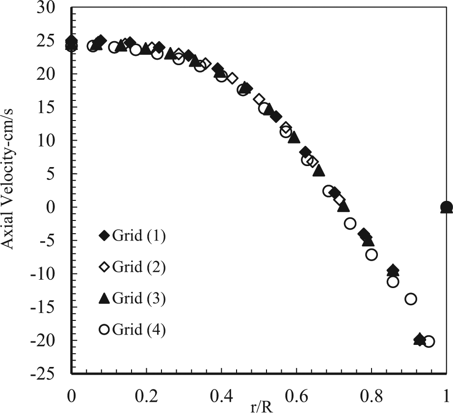
Grid sensitivity check for four different grid sizes.

Problem schematic for zero-gravity flow.
Bubble coalescence undergoing forced rotation in zero gravity
As discussed before, in the “Introduction” section, coalescence undergoing rotational force holds the key to control the bubble aggregation. Currently, the understanding of the low-gravity bubbles coalescence behaviour is limited. It is widely accepted that bubble break-up contributes to changes in the bubble size distribution, but this is considered to be negligible for either small bubbles or for Marangoni flow because of zero buoyancy force. Colin et al. 37 and Kamp et al. 38 among other workers 25 reported no bubble break-up for the whole range of operating conditions studied in the turbulent regime. Therefore, in the present work, a purely coalescing mechanism for bubble growth will be considered and the extent to which coalescence occurs is discussed. A rotating bubble column with varying rotational speed of 0.25, 0.5, 0.75 and 1 rad/s about its axis of symmetry is considered.
Figure 4 shows the schematic representation of the air–water bubble column of diameter 120 mm and height 120 mm. The properties of air and water used in the simulation were taken from ANSYS Fluent 30 (see Table 2). The geometry consists of air with a constant speed of 1 cm/s flowing through a 30 mm inlet from the bottom of the water column. The inlet velocity was chosen to be close to the velocity of gas in zero-gravity, thermocapillary flow. 23 The geometry was modelled as 2D axisymmetric to reduce the computational time. Part of the upper surface (top wall) of the domain was set to pressure outlet; the rest of top and bottom walls were defined as no-slip solid walls (see Figure 4 for details).
Coalescence occurs instantaneously after two bubbles collide forming a new sphere. Bubble collision and coagulation lead to a reduction in total number concentration. However, the total bubble volume remains unchanged. The coalescence rate can be expressed as the product of collision frequency and coalescence probability. Collection kernels used for the population balance modelling are complex and have not yet been benchmarked for zero-gravity environments. A number of applicable kernel models for the determination of bubble coalescence in thermocapillary flow are available. Two coalescence kernels suggested by a number of authors for small bubbles diameter and laminar shear collision mechanisms will be implemented in this investigation.
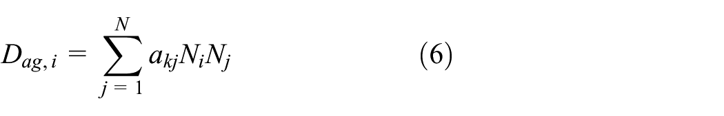
The aggregation kernel for laminar flow (model A)
The aggregation kernel

where
The aggregation kernel for Laminar shear flow (model B)
Bubbles in a uniform laminar shear flow collide because of their relative motion. In modelling the bubble motion, in laminar shear flow, its motion is assumed to be rectilinear. For this case, the collision frequency function
where
Results and discussions
Simulations are performed to study the influence of changing the column rotational speed on bubble coalescence in zero gravity where air is entering from the bottom of the rotating column. A thorough study of the effect of rotational speed on bubble size distribution using two coalescence kernels for laminar flow is reported. The study begins by investigating the dependence of the aggregation kernel. Classes were assigned such that n = 4, that is, the volume of class i + 1 is four times the volume of the previous class i (vi + 1 = n·vi). A six different bubble size groups used for the PBM simulation of the bubble column are given in Table 5. Both collection and aggregation kernels were implemented in the CFD using special UDFs.
Assigned bubble sizes of n = 4 for the population balance simulation.

Air phase development
Figure 5 shows the air phase development inside a column rotating at 0.5 rad/s and the inlet gas velocity was set equal to 1 cm/s (approximately close to the thermocapillary migration velocity of same bubble size diameter), at four time steps, namely 4, 14, 24 and 34 s. Based on the considered angular velocity, each turn requires about 12.566 s. Thus, those four time steps produce 0.32, 1.11, 1.91 and 2.71 turns. Vertical and horizontal axes represent the column height and diameter. Under the current operating conditions, a quasi-steady state was reached after 30–40 s (about three turns) of real-time simulations. A typical percentage of bubble diameter columns for the same case and time steps (used in Figure 5) are shown in Figure 6, which indicates a coalescing mechanism for bubble growth during the flow until it reaches the steady-state condition, that is, after 34 s. This is illustrated by a reduction in the small size (1.2 mm) diameter (from over 75% to less than 40%) and increase in the large-size (6 mm and above) diameter (from less than 25% to greater than 60%). Figure 6 shows that the bubbles are not formed a distribution with a range of sizes in the bubble column, but rather narrow range. Thus, it cannot be represented with Sauter mean diameter as this model considers that several bubble groups with different diameters to be represented by an equivalent phase.
Air phase (1 cm/s) development inside a rotating column (ω = 0.5 rad/s): (a) time = 4 s, (b) time = 14 s, (c) time = 24 s and (d) time = 34 s.

Percentage distribution of bubble diameter in a rotating column (ω = 0.5 rad/s) and air flowing at 1 cm/s in zero gravity.
Figure 7 presents the density distribution as a function of bubble sizes at time steps of 4, 14, 24 and 34 s, for the same stated case. The typical number density (ND) of bubble size inside the rotating column shows the development of number density with the time until steady state attainment after about three turns (Figure 7). That is as the time step increases, there is an increment in the number density of larger (right) and smaller (left) bubble sizes, which shows the bubble coalescence and creation, respectively. Also, as the time step is increased, bubbles undergo coalescence which results in a sharper (low variance) bell-shaped distribution. It should be noted that ND is a function of coalescence process only.

Number density at various time steps for ω = 0.5 rad/s.
Effect of rotational speed
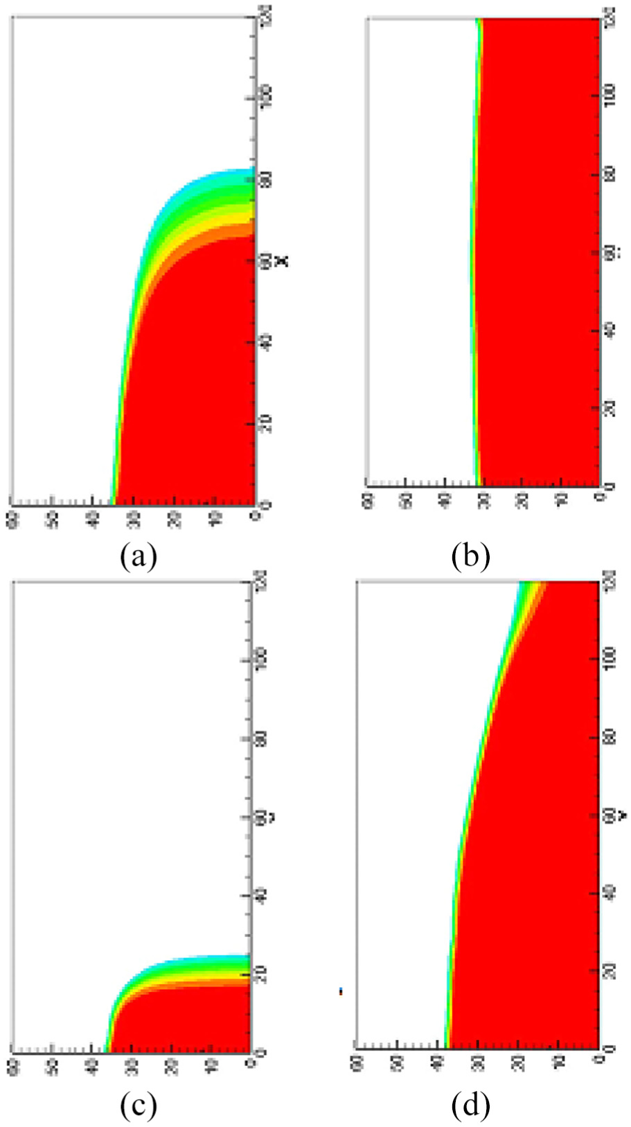
The simulation results shown in Figure 8 are presented for five different rotating speeds (0, 0.25, 0.5, 0.75 and 1 rad/s) at a fixed air inlet velocity equal to 1 cm/s. Comparison between cases in a vertical column indicates the effect of time step, at constant speed, and comparison between cases in horizontal row indicates the effect of rotational speed on the development of the air phase. These cases in Figure 8 reveal that there is a significant influence of the rotational speed on the migration of air phase, that is, rotating the column not only causes bubble collision but also accelerates the speed of moving bubbles throughout the column. It is clear that the centrifugal force (for rotating cylinder) is pulling the bubbles towards the axis of rotation and shifts them away from the wall (refer to Figure 8 for 0 and 1 rad/s). This is confirmed by narrower distribution along the column diameter and higher along the column height as the rotational speed increases, for all time steps. In Figure 8, it is observed that for 1 rad/s at t = 20 s, the column was in a complete fluidization state unlike at lower rotational speeds. However, the comparison in vertical column indicates the development of the air phase with time, as described in Figure 7.

Effect of different angular speed in zero gravity on the transient development of air flow at 1 cm/s.
A typical bubble number density column is shown in Figure 9 for both tested coalescence models. It is clear that both kernels for laminar flow (model A) and laminar shear flow (model B) produced equivalent number density at all rotational speeds. This is confirmed by the close agreement of symbol data points (model B) and the continuous lines (model A) at bubble diameter of 0.6 cm. Figure 9 shows developments in the parabolic shape around the centerline of the column due to centrifugal force effect in the air phase for different rotational speeds. The results indicate that rotation reduces the turbulence dissipation coming from the wall and could help in moving the gas phase as shown in the changes in the parabolic shapes. As the rotational speed is increased, bubbles undergo coalescence, which results in a sharper (low variance) bell-shaped distribution (Figure 9). In general, the number density decreases as the rotational speed increases. It should be noted that the number density is a function of axial position in the column owing to the coalescence process.
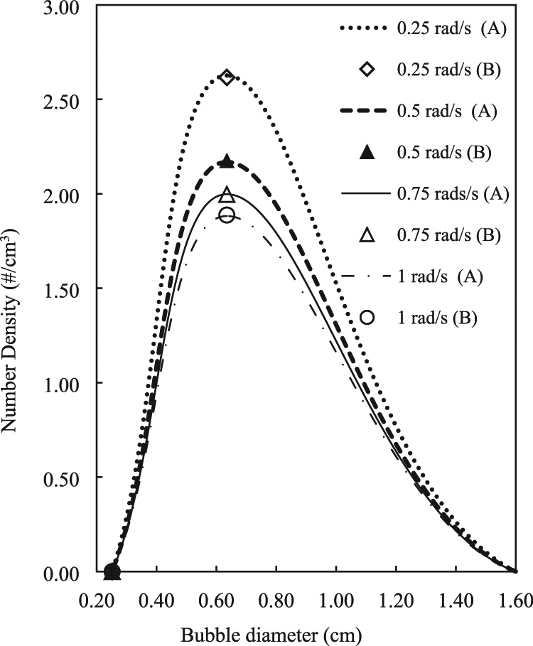
Comparison between the two kernels model for air inlet = 1 cm/s.
Another study has been conducted to investigate the size distribution of the bubbles due to change in the n classes of the PBMs. As mentioned earlier, the determination of bubble size is based upon the bubble volume interval where the index i refers to the bubble size group. The new value is assigned such that the volume of class i + 1 is related to the volume of the previous class i (vi + 1 = x·vi). Assigned bubble sizes of n = 2 and n = 4 for the population balance simulation is listed in Table 6. The bubble number density of air entering the column at 1 cm/s is presented in Figure 10 for bubble sizes of n = 2 (left side) and n = 4 (right side). Comparing the results in Figure 10 shows that the PBMs produced similar trends with different magnitude of bubble diameters and number density for different bubble size groups. In general, lower class (n = 2) has a smaller bubble diameter and a much larger number density than those obtained for the higher class (n = 4). It should be stated that the gas volume equals the number density multiplied by the volume of gas bubbles, that is, an inverse relation is existed between number density and bubble diameter for constant volume of gas.
Assigned bubble sizes of n = 2 and 4 for the population balance simulation.


Number density for bubble sizes of n = 2 (left) and n = 4 (right).
Effect of air inlet velocity
Simulations are performed for four different air superficial velocities of 1, 2, 3 and 4 cm/s, while the rotational speed was set constant at 1 rad/s. This is done to study the influence of changing air inlet velocity on bubble coalescence in zero gravity and to predict air inlet velocity effect on the particle size distribution. Figure 11 presents the density distribution as a function of particle sizes at the four stated air inlet velocities and for class n = 2 show increase in number density with increase in air inlet velocity. As the air inlet velocity is increased, bubbles undergo coalescence, which results in a large-variance bell-shaped distribution (Figure 11). This demonstrates that the bubble diameter depends on air velocity through the column inlet.
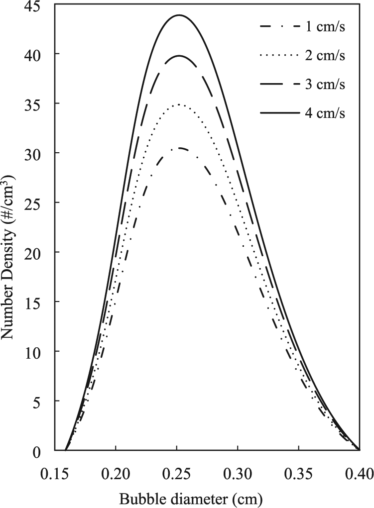
Number density for different air inlet velocity.
Figure 12 shows the effect of air inlet velocity on the air bubble size distribution. This was performed by comparing the number density (#/cm3) at the inlet velocities of 1, 2, 3 and 4 cm/s. Figure 12 shows a decrease in smaller and an increase in larger bubble with an increasing inlet air velocity, even though all simulations were started with the initial particle size equals to 1.2 mm and a constant growth rate. This is evident as the initial diameter decreases from about 43% at 1 cm/s to less than 28% at 4 cm/s and bubble agglomeration increases from about 54% at 1 cm/s to less than 68% at 4 cm/s. However, all simulations show that bubbles are formed with limited size distribution in the bubble column. Therefore, this model cannot be represented by an equivalent phase with the Sauter mean diameter dg.

Effect of different air inlet velocity on the bubble size distribution: (a) air inlet velocity = 1 cm/s, (b) air inlet velocity = 2 cm/s, (c) air inlet velocity = 3 cm/s and (d) air inlet velocity = 4 cm/s.
Conclusion
Euler–Euler simulation of air–liquid flow in a bubble column has been coupled with a population balance equation. Coalescence and break-up phenomena have been taken into account under normal gravity during validation of the model using bubbles distributed into six diameter classes. Only coalescence phenomenon has been considered under zero-gravity condition, for each class. Based on the reported results, the following conclusions may be drawn:
CFD can be used as a reliable tool to gain more knowledge and a detailed understanding of the hydrodynamics of bubble column under zero-gravity conditions.
The examined two kernel models (one for laminar flow and the other for laminar shear flow) show no difference in the obtained data. Thus, a constant value for Kernel in zero gravity could be obtained and assigned for population balance modelling for future work.
The population balance under rotational effect for turbulence and in normal gravity is different than that for zero gravity and laminar.
PBMs produced comparable results for different bubble size groups (similar trends with different magnitude).
Rotation has a significant impact as it enhances the bubble collision and helps in accelerating the speed of bubble motion throughout the column under zero gravity.
The centrifugal forces (for rotating cylinder) are pulling the bubbles towards the axis of rotation and shift them away from the wall (reduces the turbulence dissipation coming from the wall and help in moving the gas phase).
Increasing the inlet air velocity shows an increase in the coalescence rate with a decrease in the inlet bubble diameter.
Under zero gravity, the bubbles are formed with limited size distribution and may not be represented by an equivalent phase with Sauter mean diameter.
Footnotes
Appendix 1
Handling Editor: James Baldwin
Declaration of conflicting interests
The author(s) declared no potential conflicts of interest with respect to the research, authorship and/or publication of this article.
Funding
The author(s) received no financial support for the research, authorship and/or publication of this article.