
Abstract
To accurately determine the temperature-dependent parameters of composites, a thermo-elastic parameter identification approach using thermal modal data is proposed in this article. The investigation is based on two hypotheses: (1) the structure is at steady-state temperature field, which means the temperature distribution is time independent; (2) temperature distribution can be determined in advance of thermo-elastic parameter identification, and thermal-related large deformation is not considered. The thermal-dependent elastic constants and thermal expansion coefficients are expressed as intermediate functions with the independent variable of temperature, perturbation method is adapted to calculate the sensitivity of thermal modal frequencies with respect to the intermediate variables, and variables with high sensitivity are selected as the identifying parameters. By constructing the intermediate function and calculating the relative sensitivity, thermo-elastic parameters are identified by minimizing the residual between experimental and analytical natural frequencies under thermal circumstance. Two different types of composite models are employed to verify the strategies of parameter identification. Results show that on the basis of the intermediate function, the proposed approach can be applied to identify the thermo-elastic parameters effectively.
Keywords
Introduction
High temperature and temperature gradient have great influence on the dynamic performance of composite structures, 1 design of which is based on the mechanical property of composites. Elastic parameters of composites under thermal circumstance vary with temperature, and determination of these material parameters has drawn much interests.
Thermal structural dynamics has been widely investigated by theoretical analysis, numerical simulation, and experimental measurement. Savoia and Reddy 2 studied multilayer plate under heat and mechanical loads in the context of quasi-static hypothesis. Mukherjee and Sinha 3 analyzed the dynamic thermal response of thick laminated composites using finite element method. Matsunaga 4 presented a global high-order theory for solving the free vibration problem of the sandwich plates subjected to thermal loading. Meanwhile, heat will cause thermal expansion of the structure. The expansion will produce thermal stress inside the structure and affect the mechanical performance of the structure. 5 Therefore, it is of great theoretical and technical significance for the study on the thermo-elastic behavior of composites. Experimental measurement and theoretical analysis are the major approach for predicting thermo-elastic parameters. Gao et al. 6 referred to the test specification of E228-1 in ASTM, using dilatometer to measure the thermal expansion coefficient of two-dimensional (2D)-woven and three-dimensional (3D)-braided composites from 35°C to 800°C. Pan et al. 7 tested the longitudinal compression performance of 3D-braided composite materials using the separated Hopkins pressure rod combined with the heating device, material mechanical properties, and thermal physical properties were obtained in the range of 23°C–210°C. Schapery 8 deduced the bounds of the effective thermal expansion coefficient of isotropic and anisotropic composites using the principle of thermal elasticity.
The identification of composite material parameters belongs to the category of inverse problem.9,10 Sepahvand and Marburg 11 developed an inverse stochastic method based on the non-sampling generalized polynomial chaos method for identifying uncertain elastic parameters from experiment modal data. Multi-scale method is an important method to predict the cyclical composite parameters. However, the modeling of cells is complex, and the composites in the preparation will also lead to different shapes. Chen et al. 12 determined the thermoelastic parameters of braided composites and established the 2.5D cell model. Qin et al. 13 and Fei et al. 14 identified the thermal-related parameter of braided composites at high temperature. A large number of parametric modeling of different periodic composites are also carried out in previous studies.15–19
Model updating-based parameter identification has been widely applied in engineering. 20 Researchers have paid much attention in recent years to the field of structural parameter identification using experimental modal data.21–26 Experimental frequency response function combined with modal data were used to identify the damping matrix.27,28 The response surface model as a surrogate model for identifying the elastic parameter can be found in previous studies.29–31 Substructuring-based model updating has better performance in efficiency for complex structures. 32 However, there are few studies on the identification of mechanical behaviors of composites at high temperature.
Assuming that the structural dynamic performance is uncoupled with temperature, high temperature environment affects the structural vibration response non-reversing. According to the above hypothesis, the temperature distribution and structural dynamic characteristics of the structure at high temperature are separated. The accuracy of the structural dynamics model in high-temperature environment is composed of structural temperature distribution and structural dynamic characteristics.
In this article, thermo-elastic parameters are identified using finite element model updating.33,34 The elastic constants and thermal expansion coefficients are expressed as intermediate functions with the independent variable of temperature, perturbation method is adapted to calculate the sensitivity of thermal modal frequencies with respect to the intermediate variables, and variables with high sensitivity are selected as the identifying parameters. Minimizing the discrepancy between calculation and experimental thermal modal data is the objective function. The process of identifying thermo-elastic parameters is transformed into an iterative solution to the optimization problem.
Basic theory
Free vibration of thermal composite structures
Under thermal circumstance, the free vibration equation of the composite structures without considering damping is given as

and the generalized eigenvalue formula is

where

in which the first part
The generalized Hooke’s Law of orthotropic material under thermal circumstance is

where
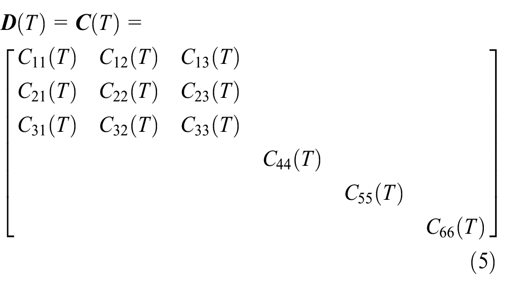
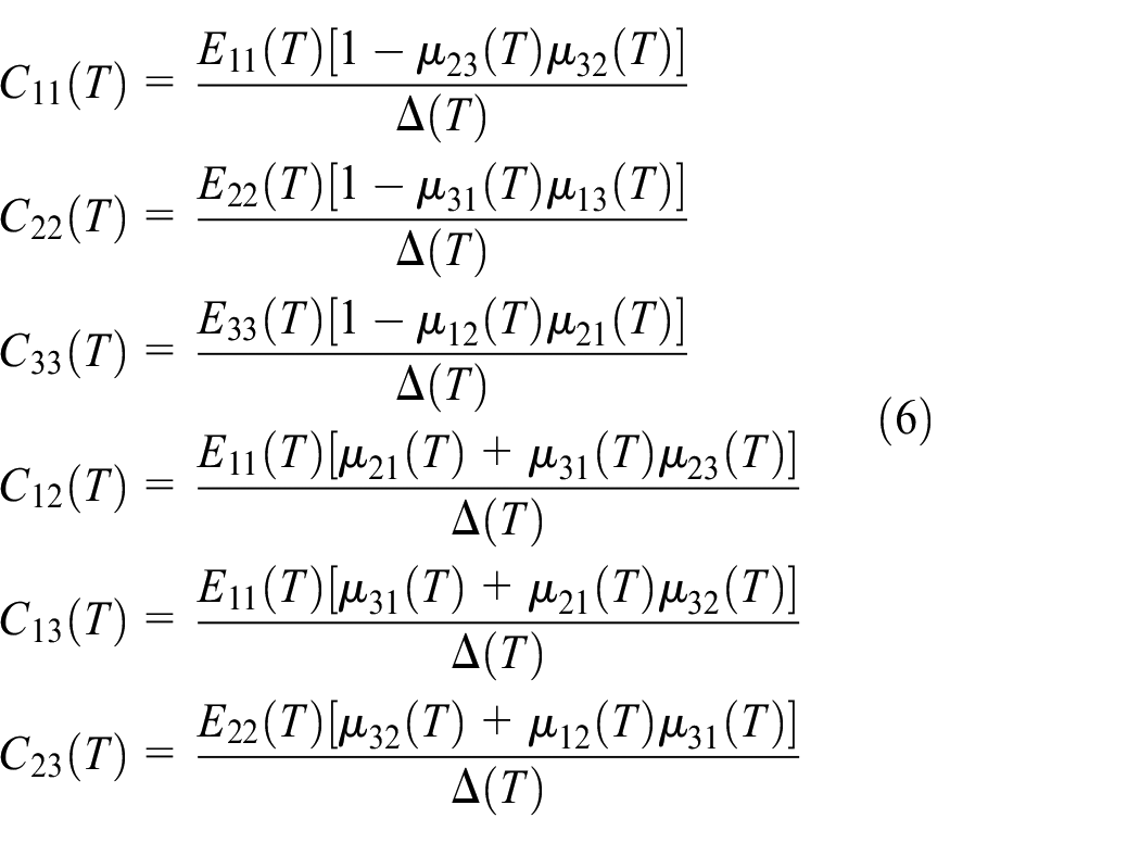
where

and the shearing stiffness are


in which ψ is the transient or the steady-state temperature field, ψ0 is the initial temperature field, and α1, α2, α3 is, respectively, the coefficient of thermal expansion in three different directions. Composite material properties such as the elastic parameters and the thermal expansivities are always varying with temperature, using letter P to represent the temperature-dependent parameter and which can be expressed as 35

where V0, V–1, V1, V2, and V3 are the coefficients of temperature, which is treated as an intermediate variable for parameter identification.
Using the principle of minimum potential energy to deduce the stiffness matrix

where Ω is the integration domain,
For the free vibration problem, the potential energy in domain Ω of the external force is zero because the structure is not loaded. The total potential energy in the volume is

According to the principle of minimum potential energy

Substituting equation (11) into equation (13)

in which the first part is the stiffness matrix

and the second part is the nodal force deduced by temperature and can be expressed as

Substituting equations (15) and (16) into equation (14), the equilibrium equation is obtained

By solving the thermal induced deformation problem (equation (17)), we can obtain the nodal displacement δe, and the deformation will cause additional stiffness effects on the structure, which is the so-called thermal stress stiffness matrix and can be expressed as

where

From the formula derivation, by substituting equations (15) and (18) into equation (3), the stiffness matrix

By substituting equation (20) into equation (2) and solving the eigenvalue problem Peig(λ,

It is shown that λ and
Identification of thermo-elastic parameter
Parameter identification
Using structural response to identify the material parameters is an inverse procedure, and an optimization problem is formulated with the objective function of minimizing the discrepancies between the numerical and the experimental modal data and is defined as

where J(

When only taking temperature-dependent composite material parameters into account and neglecting other effects, assuming the mass distribution is accurate, modal parameters can be presented as function of the coefficients

where

The parameter identification problem (equation (22)) is transformed as

Using the sensitivity analysis method to solve the optimization problem (equation (26)), the jth iteration step can be described as

in which the superscript (j) indicates the jth step in the iteration. For parameter identification,

in which
For solving the linear algebra equations (equation (27)), the identified parameters at the jth iteration step are obtained as

in which

After the convergence of
Sensitivity analysis
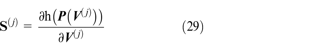
Calculating the sensitivity matrix

where
Modal frequencies and mode shapes are two parts contained in the selected structural responses
The coefficient vector of temperature-dependent parameter is represented by equation (25), and according to equation (10), and different material parameters are always with different coefficients, the identifying coefficients vector is

in which

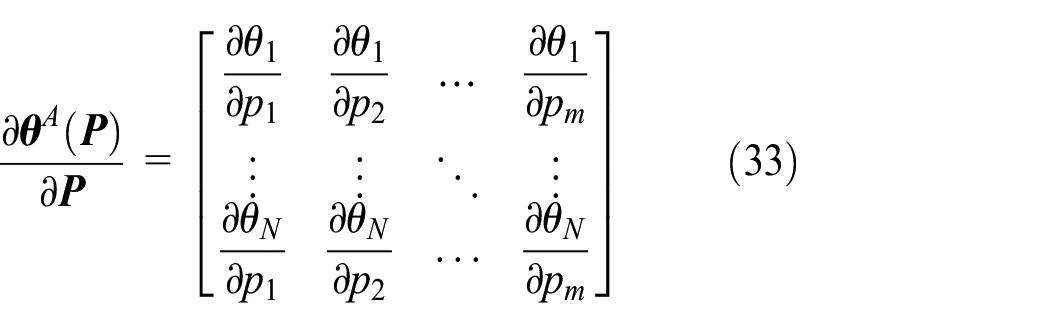
The sensitivity matrix of the modal parameters with respect to the coefficients is

in which
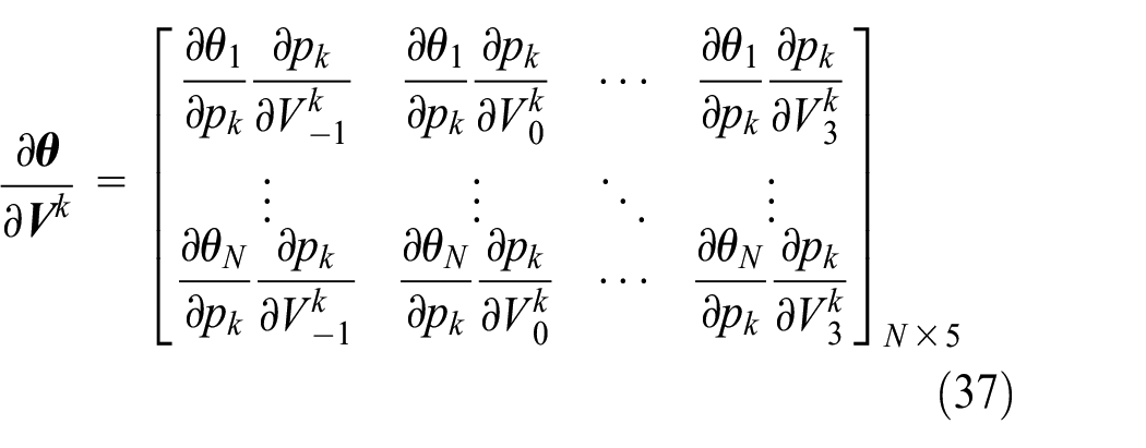
Therefore, the dimension of the sensitivity matrix is N row, 5×m column. If the relationship between material parameters and temperature is not complicated, the dimension can be reduced. Due to the structural responses,
In the process of finite element analysis, the local stiffness matrix and local mass matrix of a single element are generated by the physical parameters such as geometry, material and properties of each element, and then assembled into the global stiffness matrix and mass matrix of the structure. According to equation (2), the differential equation for the parameter
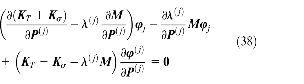
The sensitivity matrix of eigenvalues with respect to material parameters can be obtained

Similarly, sensitivity matrix of mode shapes with respect to material parameters in the structure can also be obtained. The advantage of intermediate variable method is that it can effectively characterize the relationship between composite material parameters and temperature, and the temperature-dependent thermo-elastic parameter identification is transformed to identify the coefficients of the intermediate variables.
Implementation procedure
This article presents a parameter identification method of structural dynamics model at high temperature. Because the material parameters (coefficient of thermal expansion and other parameters) are temperature-dependent, the relationship between the parameter and the temperature is expressed as the intermediate function at different temperature conditions. Then, the coefficients of the intermediate function reduce the number of parameters to be updated. Main steps are as follows:
According to the geometric parameters and the initial material parameters, the initial finite element model is established to calculate the thermal mode parameters at high temperature.
The relationship between the material parameters and the temperature is assumed to be an intermediate function, the coefficient of which is determined as the intermediate variable.
The relative sensitivity of the intermediate variables is calculated by the difference method, and the parameters to be updated are selected according to the sensitivity analysis results.
The residuals of mode frequency between simulation and experiment are constructed as objective functions, and the model are optimized by the iterative optimization until the parameters converge to obtain the structural of dynamic model at the high temperature (Figure 1).

Flow chart for the thermo-elastic parameter identification.
Case studies
Parameter identification of a homogenized composite panel
The material parameters of the C/SiC composite panel is shown in Table 1, and the elastic modulus, shear modulus, and thermal expansion coefficient of composites are varying with temperature. And the geometrical size of the panel is 400 mm × 200 mm × 4 mm, and the boundary condition and the temperature field are shown in Figure 2.
Material parameters of the composite.


Composite plate model with heat conduction direction (unit: mm).
Assuming that the temperature is evenly distributed along the length of the composite panel, regardless of the effect of air convection, the ambient temperature and the initial temperature of the composite plate are Tamb = Tinit = 20°C. The heat transfer finite element model is established using solid element in NASTRAN, which is a commercial finite element software, and the steady-state temperature field of composite panel is calculated by SOL106 solver. The temperature field was applied at 800°C on the upper side of the panel and the temperature on the lower side was 300°C. The non-uniform temperature field was shown in Figure 3. This temperature field calculates the thermal mode as a temperature load.

The steady-state temperature field under the temperature load of 300°C–800°C.
Determination of intermediate function
Since the structural stiffness coefficient is affected by the temperature in the thermal environment that the structural thermal mode are changed. The stiffness coefficients C11, C22, C33, C44 and the thermal expansivity coefficients αx, αy are chosen. The intermediate function describes the relationship between parameters and temperature.
The parameter values of the thermal expansivity αx, αy and the stiffness coefficients C11, C22, C33, C44 between 300°C and 800°C are linearly fitted by the least square method. The abscissa of the fitting curve is the temperature value, the coordinate is the parameter value, and the fitting equation is as follows

which indicates that the material parameters approximate linear distribution in the range of 300°C–800°C, t is the parameter of temperature, the equations can be written uniformly as P = kt + b, k and b is respectively the variable of the first order and the zero order of temperature.
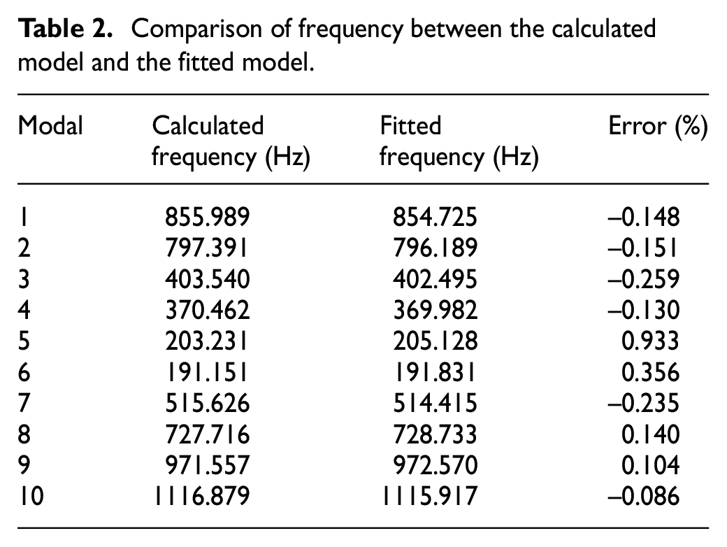
Figure 4 shows the six parameters of the linear fitting curves. The material parameters and stiffness coefficients after fitting are substituted into the recalculated thermal mode analysis. Comparison of frequency between the calculated model and the fitted model is shown in Table 2, it is found that the modes are not shifted, and the modal frequency values of the first 10 orders are with high accuracy.

The fitting curve of thermo-elastic parameters: (a) C11, (b) C22, (c) C33, (d) C44, and (e) αx, αy.
Comparison of frequency between the calculated model and the fitted model.
Parameter identification
Five parameters are selected: C11-b, C22-b, C44-b, αx-k, and αy-k, and the relative sensitivity values of which are slightly larger than the other parameters. Simulation study is conducted to verify the parameter identification procedure. Assuming the real value of C44-b is 1.2 times the initial value, and C11-b C22-b, αx-k, and αy-k are 1.08 times each of the initial value, the experimental thermal modal data are obtained by assigning the perturbed values to the corresponding parameters. The first 10 order of modes exactly match before and after the perturbation. The comparison of modal frequency between initial and experimental model is shown in Table 3, the fifth mode and the sixth mode are switched. Figure 5 shows the variation of parameters in the convergence procedure. As can been seen from the figure, after parameter convergence, the parameter variation of C44-b, C11-b C22-b, αx-k, and αy-k is 20%, 8%, 8%, and 7.8% of the initial value, respectively; comparing with this result, the perturbed value of the initial parameter is 120% of the initial value of C44-b, 108% of the initial value of C11-b C22-b, αx-k, and αy-k, the parameters are identified with high accuracy.
Comparison of modal frequency between initial and experimental model.

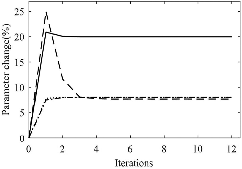
Parameters convergence (—C44-b, --- αx, y -k, -·-C11-b, ···C22-b).
In order to further testify the identification procedure, the initial parameters and its fitting curve, the perturbed parameters, the fitting equation of modified parameter are plotted together to compared. The initial fitting curves of the five material parameters C11, C22, C44, αx-k, and αy-k and the perturbation and the updated curves are shown in Figure 6. Comparison of experimental and updated modal frequency is shown in Table 4. It can be seen from the figures that the updating parameter curves are almost coincident to the curves of experimental parameters, indicating the effectiveness of parameter identification method.

The fitting curves of thermo-elastic parameters: (a) C11, (b) C22, (c) C44, and (d) αx, αy.
Comparison of experimental and updated modal frequency.

Parameter identification of a 2.5D-braided composite panel
Investigation on a 2.5D-braided composite panel is conducted, and the geometrical parameters, the temperature field, and boundary conditions are shown in Figure 7. Simulated experimental thermal modal data can be obtained using the mesoscale model, which is constructed according to the geometric model of 2.5D-braided composites and the following four assumptions: (1) the warp weft axis is a straight line, (2) weft yarns have the same cross sections, (3) no gap exists between the substrate and the yarn, and (4) the knitting angle of the yarns is the same. The volume fraction of fiber is 40%, and the weaving inclination of the warp yarns is 15°. The unit cell of the composite is shown in Figure 8, which is constructed using solid element. Based on the model of unit cell of the braided composite, the adopted model for simulation study is six times of the unit cell model which is shown in Figure 9.

2.5D-braided equivalent model with heat conduction direction (unit: mm).

Finite element model of unit cell of 2.5D-braided composites.
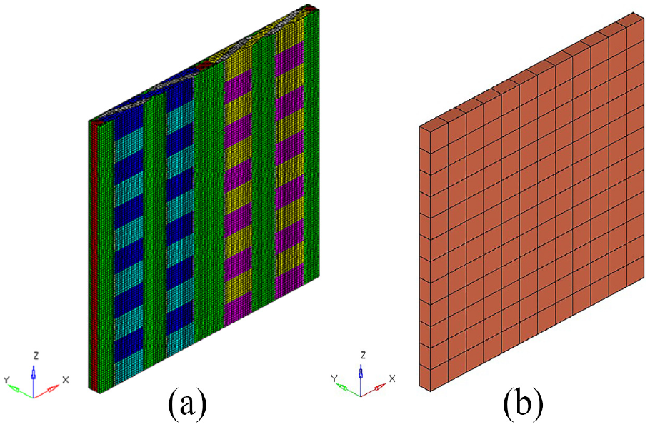
Finite element model of 2.5D-braided composites: (a) mesoscale model and (b) equivalent model.
Equivalent modeling is widely employed for composite structural analysis, and the thermo-elastic parameters and the expansion coefficient of the equivalent model are shown in Table 5.
Material parameters of the 2.5D-braided equivalent model.

Similar to the previous example, the heat transfer finite element model is established in NASTRAN. The steady-state temperature field of the composite panel is calculated. The temperature is 300°C on the lower side of the panel and the temperature on the upper side is 800°C. The non-uniform temperature field is shown in Figures 10 and 11. The thermal mode is obtained under the temperature field, and the parameters of composite in the range of 300°C–800°C are identified.

The temperature field of refine model under 300°C–800°C.

The temperature field of equivalent model under 300°C–800°C.
Determination of intermediate function
The least square method is used to fit the composite parameters, the intermediate function is constructed, and the intermediate variables are chosen as the parameters to be updated. The thermal expansivity αx and the stiffness coefficients C11, C33, and C66 between 300°C and 800°C are linearly fitted by the least squares method in which the fitting equation is as follows

Figure 12 shows the four parameters of the linear fitting curve. The initial parameter points are almost distributed in the fitting line, because the material parameter field of the yarn changes linearly with the temperature. The material parameters and stiffness coefficients after fitting are substituted into the recalculated thermal mode analysis. The thermal modal frequency of equivalent model is obtained from the initial parameters, and the equivalent results still have considerable errors.
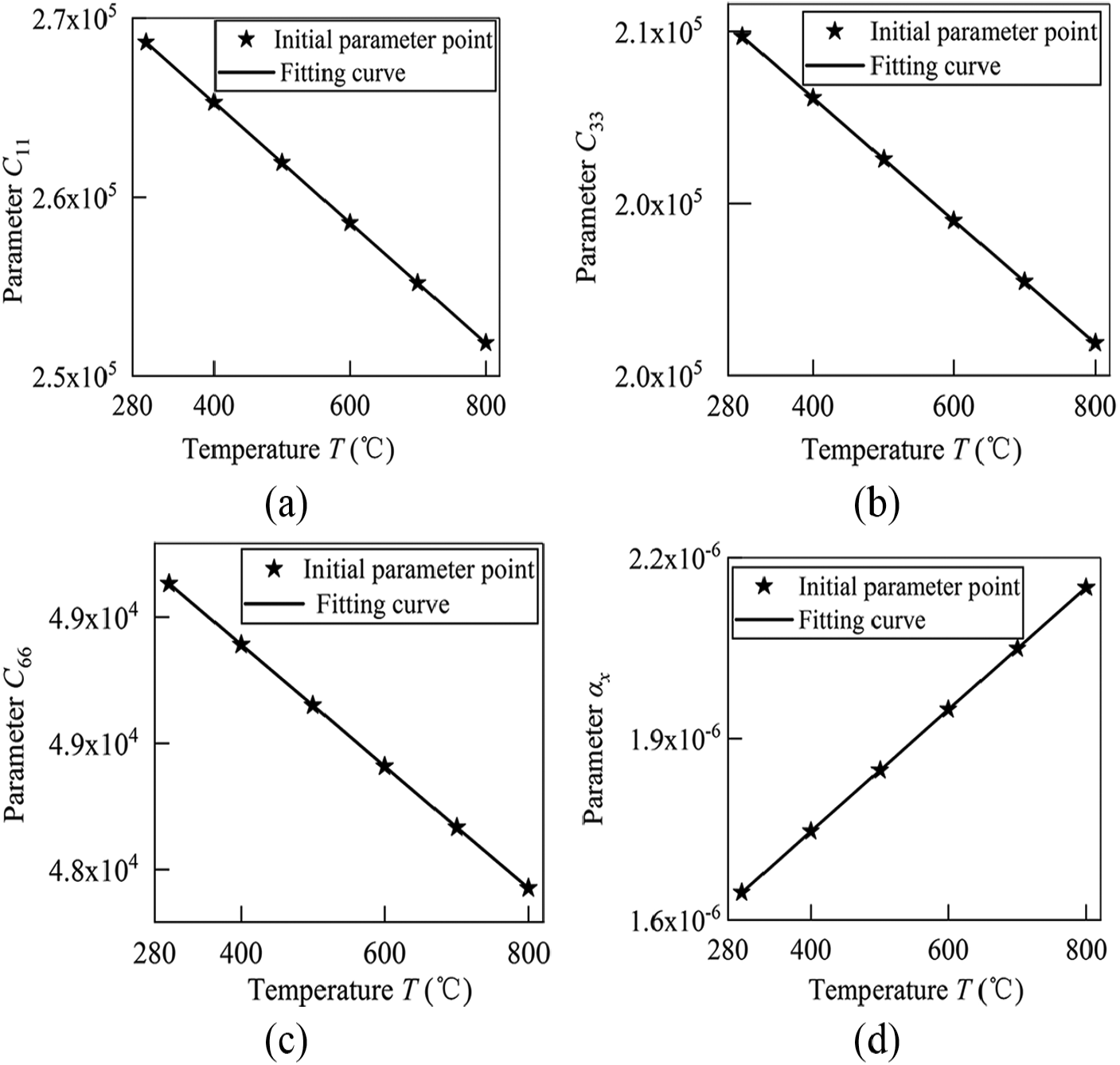
The fitting curve of thermo-elastic parameters: (a) C11, (b) C33, (c) C66, and (d) αx.
Updating parameters selection
The least squares fitting equation is assumed to be a linear relationship P = kt + b. Assuming that the slope coefficient of each parameter fitting equation is k, the intercept coefficient is b. The 24 parameters obtained by fitting the thermal expansivity coefficients and stiffness matrix coefficients are calculated by the difference method. Selecting the four parameters: C11-b, C33-b, C66-b, and the thermal expansivity coefficient αx-b, which are slightly more sensitive than the other parameters. The absolute value of the relative sensitivity result is shown in Figure 13.

Relative sensitivity absolute value.
Parameter identification
The thermal modal frequencies calculated from the refined model are treated as the experimental modal frequency. Then, the calculation and experiment of the first seven-order modal frequency as well as error is shown in Table 6, and the maximum error is 10.44%. The iterative convergence of parameters C11-b, C33-b, C66-b, and αx-b is shown in Figure 14.
Comparison of frequency between finite element model and experimental model.


Parameters convergence curve (—C66-b, --- αx-b,-·-C11-b, C33-b).
After parameter identification, the parameter variation of C11-b, C33-b, C66-b, and αx-b is, respectively, –13.66%, 9.62%, 32.22%, and 44.46% of the initial value.
Table 7 shows comparison of modal frequency between the updated and the experimental model, the maximum error of the modal frequency between the initial and the experimental model is 10.44%, and the error between the updated frequency and experimental frequency is less than 0.568%. For testing the robustness of the parameter identification method, 3% noise is added to the test data, and the error of the identified model is less than 1.34%, indicating that the parameter identification based on thermal modal frequency is effective and robust.
Comparison of modal frequency between the updated and the experimental model.
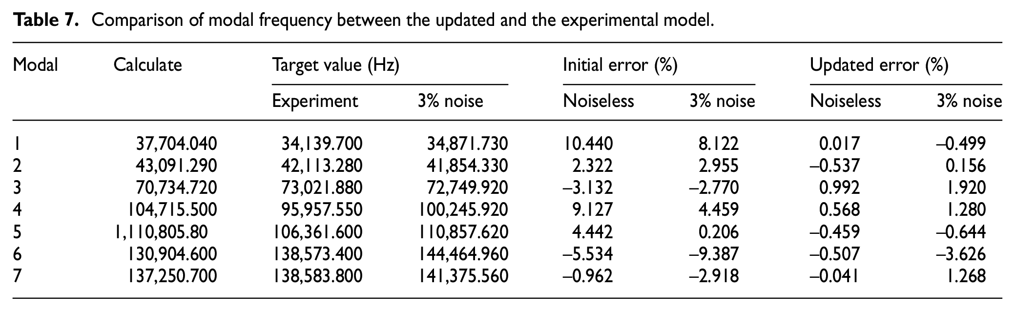
According to the case studies of the parameter identification of composites, the effectiveness of the proposed method has been testified. After parameter identification, the error of the modal data of the composite model is greatly reduced and the thermo-elastic parameter can be accurately determined, and the robustness of the proposed method is illustrated by adopting the noised experimental data.
Conclusion
An approach for composite thermo-elastic parameters identification is proposed in this article. Constructing the intermediate function for thermo-elastic parameters with respect to the temperature, the updating of undetermined coefficient will improve the calculation efficiencies. Parameter sensitivity analysis is conducted using the finite difference method. The intermediate function coefficients can be identified by minimizing the residual between the analytical and experimental thermal frequencies. The major advantage is that the proposed method will determine the thermo-elastic parameters by considering the effect of non-uniform temperature and provide a convenient method to accurately predict elastic parameters and thermal expansion coefficients of composites. The composite parameters always vary nonlinearly depending on the temperature, which will introduce difficulties into parameter identification and should be investigated in the future.
Footnotes
Appendix 1
Handling Editor: S Sfarra
Declaration of conflicting interests
The author(s) declared no potential conflicts of interest with respect to the research, authorship, and/or publication of this article.
Funding
The author(s) disclosed receipt of the following financial support for the research, authorship, and/or publication of this article: The work was supported by the National Natural Science Foundation of China (No. 11602112).