Sage Journals: Discover world-class research

Abstract

Due to the increasing number of vehicles in urban areas and the degradation of pavement performance, the failure rate of polyethylene pipeline, across roads, has increased rapidly. Based on relevant data, the traffic loads are regarded as a random variable; also its distribution is determined. First, the nonlinear contact interaction model was established, among traffic loads, soil and buried polyethylene pipeline, using finite element analysis software. Second, considering the decline of the pavement performance, the mechanical characteristics of buried gas pipeline suffering from different traffic loads were analyzed. Based on statistics of vehicle load, the distribution law of its maximum equivalent stress was determined by numerical simulation. Particularly, the strength distribution law of polyethylene pipeline was obtained through experiments. The reliability index of polyethylene pipeline was calculated using central point method and Monte Carlo method. Finally, based on the degradation curve of pavement performance, the remaining life of buried polyethylene pipeline was assessed.

Keywords

Polyethylene pipeline reliability index central point method Monte Carlo traffic loads

Introduction

As an important transportation method, the pipeline is widely used in lifeline projects, such as water supply, drainage, and gas delivery. Due to the convenient installation and maintenance, polyethylene (PE) pipeline is widely used in the transportation of urban gas. As we know, pipeline transportation uses buried form generally. There are two types of pipeline loading forms. One is internal loads (internal pressure) and the other is external load divided into natural loads and artificial loads. Buried pipelines were attacked by natural loads frequently, such as ground settlement, landslide, and debris flow.^1–3 The common artificial loads include the repeated load (traffic load),⁴ static load (surface load),⁵ impact load,⁶ and so on. Apparently, the buried pipeline in cities or towns is mainly affected by artificial loads.⁷ Especially, in recent years, with the increasing number of vehicles in urban areas and the degradation of pavement performance, the rate of failure accidents has increased rapidly. Therefore, the influence of traffic load on buried pipelines gradually becomes the research focus. The relative research on the loads, applied to pipes, has been developing since the Marston theory was put forward. At present, most researches on traffic load are focused on the response of buried pipelines or the failure of pipelines. These studies involve different types of pipes, such as concrete pipes,^8–10 steel pipes,¹¹ or flexible pipes.^12,13 In addition, these studies can also be roughly divided into experimental studies,^14–17 numerical simulation study,^18,19 and their combination.²⁰

However, the traditional design of the pipeline employs the method based on strength design criterion, such as the allowable stress. Due to the improvement of the public’s awareness of risk, more frequent natural disasters as well as the improvement of economic competitiveness, in order to meet social expectations of pipeline safety, the design and evaluation method based on the reliability must be developed.²¹ At present, the design and evaluation method based on the reliability has received a great deal of attention even if the acquisition of target reliability and relevant variables exist many problems. Many scholars have studied the reliability of pipelines, such as the study on the reliability of corroded metal pipelines,^22–24 PE pipelines with pressure²⁵ as well as buried pipelines under the external load of landslide or longitudinal ground movement.^26,27

Since the complexity in studying special material characteristics and the mechanical response of buried pipe suffering from external load, the reliability analysis of buried PE pipeline under traffic loads has not been reported. Moreover, the probabilistic assessment of an engineering system performance might contain a substantial number of uncertainties in system behavior due to its functioning mode,²⁵ which makes the reliability analysis more difficult. For buried PE pipeline under traffic loads, this uncertainty is affected by many factors, such as vehicle axle speed, coupling between vehicle, and underground pavement structure. Partial difficulties are also reflected as follows: (1) relationship assessment among the random variables of the traffic load–soil–pipeline system, (2) finding methods (or relationships) to reduce number of involved random variables, and (3) difficulty in collecting relevant data.²⁸

The aim of this work is to conduct the reliability analysis for a gas PE pipeline subject to traffic loads. Actually, once the pipeline is buried, the layered pavement structure and the form of pipe–soil contact are determined. Thus, the reliability of the pipeline is only related to external loads.^29,30 Based on the stress–strength interference model and the idea of reducing random variables, the reliability calculation of pipeline is simplified to the problem for finding the maximum stress distribution of pipeline and the strength distribution of material. Using tensile test, the characteristics of PE materials were analyzed and the probability distribution of yield strength was calculated. Numerical simulations using finite element method are performed to determine pipe–soil system response under traffic loads and obtain the relationship between traffic load and pipeline stress. Based on the statistical data of traffic loads, the probability distribution rule of pipeline stress was obtained. Based on the von Mises yield criterion, the ultimate state equation was established. Then the reliability index of pipeline was calculated using the center point method and Monte Carlo method. Finally, a graphical method of remaining life prediction based on the degradation of pavement performance is proposed to estimate the remaining life of buried PE pipeline subject to traffic loads.

Uniaxial tensile test

The real stress–strain curves of most PE pipeline are shown in Figure 1. The curve is divided into (a), (b), and (c) stages:¹ (a) the stage shows an elastic stage similar to steel; (b) this stage is the plastic softening stage or necking stage, at which the stress decreases gradually with the increase of strain; (c) this stage is the rising stage. At the end of stable necking, the stress will increase for a short time, and then, the specimen will snap. This article focuses on the change of the pipeline in the elastic stage only. Once the pipe yields, irreversible plastic deformation will occur and the pipeline will be damaged.

Figure 1.

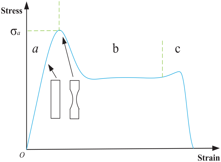
Stress–strain relationship of polyethylene material.

For the sake of uniaxial tensile test of PE pipeline materials, the sample was produced according to ISO 6259-3:2015.³¹ The tensile rate has been set as 1, 3, 10, 30, 100, and 300 mm/min, respectively. The test apparatus is shown in Figure 2. The test data are shown in Figure 3. This article only cares the data near yield. The yield strength of PE pipeline at different tensile rates (v) was calculated, as shown in Figure 4. It can be seen from the figure that the yield strength of PE pipeline has obvious rate correlation. The greater the tensile rate or strain rate, the greater the yield strength. When the strain reaches a certain degree, the greater the tensile rate, the faster the stress drops in the contraction stage. In conclusion, the relationship between yield strength and tensile rate was obtained.

Figure 2.

Uniaxial tensile test apparatus.

Figure 3.

Engineering stress–strain relationship of uniaxial tensile tests at different velocities.

Figure 4.

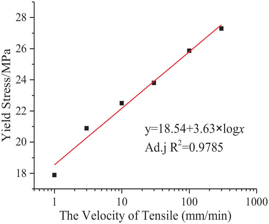
Yield stress at different velocities of tensile.

Polyethylene material is a special kind of material. Its material characteristics vary with temperature and time. Suleiman and Coree³² established a hyperbola constitutive model considering the strain rate by a more systematic method, and the curves obtained are in good agreement with the curves in Figure 3. Since this article only considers its stage before yield, this model is chosen as the constitutive model of PE pipeline materials. The general formula of hyperbola constitutive model is as follows

σ = \frac{ε}{a + b ε}

(1)

\frac{ε}{σ} = a + b ε

(2)

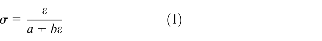
where $σ$ is the stress; $ε$ is the corresponding strain. Using equations (1) and (2), the relationship between constants a, b as well as the tensile rate v is obtained as shown in Figure 5

a = - 2.32 \times 10^{- 4} \times \log v + 6.43 \times 10^{- 4}

(3)

b = - 0.311 \times \log v + 4.26

(4)

Figure 5.

The relationship between constants a, b and the velocity of tensile.

The initial elastic modulus of PE pipeline is inversely proportional to its constant a. The relationship between them is shown as follows

E_{0} = \frac{1}{a}

(5)

Calculation of maximum pipeline stress under traffic load

Conditional hypothesis

Pipe fittings and joints of pipeline were not considered in this work.

Drucker–Prager yield criterion was used to deal with the plastic deformation of soils.

The interaction behavior between soil and pipe was a limited sliding contact.

The material properties of PE were assumed to not change over temperature and time. In other words, the creep and relaxation properties of PE would not be considered.

Material parameters

The PE80 grade pipeline was used in this work, the standard size is standard size ratio (SDR), D/t = 17.6), and the pipe diameter was 400 mm. Drucker–Prager model was adopted for soil and rigid basement soil, which can simulate the elastic–plastic state of soil under impact loads well and avoid instability in the calculation of large deformation.²¹ Because the purpose of this article is not the mechanical response of pavement structure, the cement stabilized macadam layer and asphalt concrete surface layer are regarded as homogeneous linear elastic materials. The material parameters of each layer of soil are shown in Tables 1 –3.^33,34 The density of PE pipeline was 950 kg/m³ and its Poisson’s ratio was 0.4.

Table 1.

Material parameters.

Structure	Materials	Elasticity modulus E (MPa)	Poisson’s ratio	Density $(ρ)$	Cohesive force C	Expansion angle
Rigid basement	Rock	8 × 10⁴	0.25	2600	2100	45
Filling soil layer	Compacted earth	8.5	0.35	1600	30	20
Cement-stabilized macadam layer	Cement-stabilized macadam	1000	0.3	2000	–	–
Asphalt concrete layer	Asphalt concrete	1200	0.3	2400	–	–

Table 2.

Soil modeling parameters (D-P model).

Name	Elasticity modulus (MPa)	Poisson’s ratio	Density (kg/m³)	Frictional angle	Expansion angle	Flow stress ratio
Soil	20	0.4	1867	36.5°	0°	1

Table 3.

Hardening parameters of Drucker–Prager soil.

$σ_{1} - σ_{3}$ (kPa)	$ε_{p}$
170.1	0
649.9	0.035
740.3	0.050
801.4	0.073
848.0	0.091

The failure criterion is the basis for judging the failure, which depends on the failure mode. In this article, the criterion of the von Mises yield criterion was adopted, that is, when the equivalent stress of pipeline reaches the yield stress of pipe material, the pipeline failure is considered. The equivalent stress is von Mises equivalent stress,³⁵ and its expression is

σ_{eq 4} = \sqrt{\frac{{(σ_{1} - σ_{2})}^{2} + {(σ_{2} - σ_{3})}^{2} + {(σ_{1} - σ_{3})}^{2}}{2}}

(6)

where $σ_{1}$ , $σ_{2}$ , and $σ_{3}$ are three principal stresses of a unit body, and $σ_{eq 4}$ is equivalent stress. The equivalent stress of von Mises should be less than the yield stress $σ_{y}$ .

Model establishment

The whole road model was simplified into four layers, including rigid basement, filling soil layer, cement stabilized macadam layer, and asphalt concrete layer. The pipeline was away from the pipeline side boundary more than six times the pipe diameter. The length and depth of the foundation of the model were set large enough to minimize the impact of boundary conditions. The calculation model is shown in Figure 6.

Figure 6.

Model sketch.

The entire model was a cuboid with a scale of 8 m × 6.5 m × 3.5 m, which simulates a common single lane with a width of 3.5 m.³³ Due to the symmetry of loads, semi-model was adopted for modeling. The bottom of the soil remained fixed in all direction (Ux = Uy = Uz = 0). The upper surface of the soil was free surface without any constraints. Symmetrical boundary was imposed on the other surfaces of the soil and the both ends of the pipeline, as shown in Figure 7. At the moment, the pipeline–soil contact model is the most accurate method for evaluating the interaction of the pipeline–soil at the large deformation segment and can explain the friction and separation of the pipeline–soil interface. The contact between the outer surface of the PE pipeline and the surrounding soil was set as a limited-slip contact. A contact algorithm was employed to simulate the interface between the outer surface of the pipeline and the surrounding soil. Interface friction had been taken into account in the contact algorithm in the form of defining an appropriate friction coefficient. The friction coefficient equals to 0.18.²⁶ Eight-node and hexahedron linear shrinkage integral unit (C3D8R) were employed for modeling both pipeline and surrounding soil. The mesh of the soil around the pipeline was a local mesh refinement, as shown in Figure 7.

Figure 7.

Finite element model of (a) the refined mesh around pipeline, (b) the boundary conditions, and (c) the meshing of pipeline.

Numerical calculation

Relevant regulations stipulate that the buried depth of PE pipeline under the road should not be less than 0.9 m.^36,37 When the buried depth is set as 1 m and the change range of vehicle loads (T) is 0.4–1.8 MPa, the mechanical characteristics of PE pipeline under traffic loads are analyzed; also the distribution law of its maximum equivalent stress is determined.

It can be seen from Figure 8(a) and (b) that the road is obviously deformed under the action of vehicle. By comparing to all the results, corresponding stress concentrations appear in the middle of the model, and meanwhile, the deeper the dent is, the greater the equivalent stress value it will be as the loads increase. As shown in Figure 8(c), a large deformation and stress concentration emerge in the middle of the PE pipeline, and the maximum equivalent stress appears at the lower side of the inner surface of the middle pipeline. By comparing all the calculated results, it can be found that as the action increases, the deformation of pipeline grows and the stress values strengthen and concentrated.

Figure 8.

Stress nephogram of model and pipeline (traffic load = 1.8 MPa, E₁ = 120 MPa, E₂ = 100 MPa): (a) whole model, (b) soil and pavement, and (c) pipe.

It is notable that the complex change of pavement performance is simplified into the reduction of the elastic modulus of road material in this article. As for obtaining the relationship between the stress or strain of PE pipeline and traffic loads, the calculated results are plotted into Figure 9, of which E₁ and E₂ represent the elastic modulus of asphalt concrete layer and cement stabilized macadam layer, respectively. Figure 9 shows that the maximum equivalent stress of the pipeline increases along with the raise of the vehicle loads and the aging of the pavement materials. However, due to the pipeline internal pressure, the maximum equivalent stress will not be lower than a certain value.

Figure 9.

Stress versus vehicle load.

The curve of buried pipe stress and load under traffic load was fitted to obtain the mathematical expression of the relationship between traffic load and stress. The curve was fitted with the following function, and the relevant fitting parameters were listed in Table 4

S_{T} = a + b \times T^{c}

(7)

where S_T is pipe stress (MPa); T are traffic loads (MPa); a, b, and c are coefficients.

Table 4.

Fitting of the relationship between pipe stress and traffic loads.

Elastic modulus of pavement structure (MPa)	a	b	c	Adj. R²
E ₁ = 12, E₂ = 10	6.15594	9.53034	1.51268	0.9993
E ₁ = 60, E₂ = 50	6.14192	6.81208	1.51572	0.99787
E ₁ = 120, E₂ = 100	6.5521	4.79898	1.82252	0.99713
E ₁ = 240, E₂ = 200	6.58443	3.3225	2.14823	0.99596
E ₁ = 480, E₂ = 400	6.47642	2.41642	2.41255	0.99505
E ₁ = 720, E₂ = 600	6.41911	2.08512	2.52987	0.99477
E ₁ = 960, E₂ = 800	6.38547	1.91862	2.59198	0.99468
E ₁ = 1200, E₂ = 1000	6.36479	1.81785	2.63202	0.99458

Calculation of pipeline reliability

Distribution law of vehicle loads

In terms of probability distribution characteristics of vehicles, a lot of studies on vehicle loads have been made domestically, including normal, exponential, and lognormal distribution. The multi-peak model can be simplified into a combination of normal distribution for different types of vehicle loads.³⁸ The characteristic parameters of traffic loads distribution, which obtained by Wang based on actual measured data, are used in this article.³⁹ Specifically, China’s freight cars at present mainly use tires of 9.00-20 (about 15%), 10.00-20 (about 25%), 11.00-20 (about 40%), and 12.00-20 (about 15%). These four types of tires are selected as vehicles; their specific statistical data are shown in Table 5, and the statistical data of wheel pressure of large- and medium-sized buses are shown in Table 6.

Table 5.

Statistical table of freight car load.

The front wheel of 11.00-20	Measured value	0.77	0.78	0.98	1.02	1.04	1.12	1.16	1.17	1.2	1.22	1.24
	Count	1	1	1	4	3	8	7	5	2	1	1
The rear wheel of 11.00-20	Measured value	1.20	1.22	1.24	1.27	1.29	1.31	1.32	1.33	1.35	1.36
	Count	1	2	5	7	10	8	7	5	1	1

Table 6.

Statistical table of bus load.

Large bus	Measured value	0.72	0.78	0.83	0.88	0.92	0.94	0.96	0.98	1.00	1.05	1.07	1.12
	Count	1	1	1	3	6	9	7	9	4	7	2	1
Medium bus	Measured value	0.66	0.69	0.71	0.76	0.78	0.80	0.82	0.86	0.90	0.93	0.94	0.96
	Count	1	1	4	3	5	9	7	8	6	3	5	2

The data in Tables 5 and 6 are calculated by the numerical calculation tool MATLAB. The t-test method is used to determine whether the tire pressure is normally distributed. If it is normally distributed, its characteristic parameters are given, as shown in Table 7.

Table 7.

Characteristic parameters of tire pressure distribution.

Vehicle type	Mean	Square deviation	s
The front wheel of 11.00-20	1.10	0.0114	0.9981
The rear wheel of 11.00-20	1.29	0.0011	0.9973
Large bus	0.94	0.0145	0.9790
Medium bus	0.82	0.0101	0.9996

The judgment parameter of normal distribution is h. When h = 0, it means that the original hypothesis cannot be rejected at the set significant level—the sample is subject to normal distribution. When h = 1, it means that the original hypothesis can be rejected at the set significance level—the sample is not subject to normal distribution. s is the probability when the hypothesis is true in the test. When it is small, the original hypothesis could be problematic. Therefore, the front wheel of 11.00-20 is subject to N∼ (1.10, 0.112), the rear wheel of 11.00-20 is subject to N∼ (1.29, 0.032), a large bus is subject to N∼ (0.94, 0.122), and a medium bus is subject to the normal distribution of N∼ (0.82, 0.12).

Yield strength distribution

Considering the rate correlation of PE material, when at a temperature of 23°, stretch rate is 50 mm/min and sample size is 214; pipeline tensile tests are conducted according to ISO 6259-3:2015; also the yield strength of PE80 pipeline material is obtained by statistics, as shown in Figure 10. According to the final experimental data, its yield strength follows the normal distribution of N∼ (21.13, 2.172).

Figure 10.

Histogram of yield stress frequency distribution of PE pipeline materials.

Reliability calculation

The reliability of PE pipeline can be defined as the probability that the pipeline meets demands for gas supply under specified environmental conditions. The stress–strength interference model insists that if the stress interferes with the allowable strength of the system, the system might fail.⁴⁰ As for fracture failure, the system reliability R is the probability that the strength is greater than the stress, which can be expressed as

R (t) = 1 - P = 1 - P (S - R \geq 0) = P (R - S > 0)

(8)

In the formula, P stands for the failure probability; S and R represent stress and strength distribution, respectively, and all of them are random variables with certain statistical distribution laws. The central point method in the first-order second-moment method (FOSM) was used to calculate the reliability index to establish the function of buried PE pipeline structure under traffic loads

Z = g (X_{1}, \dots, X_{i})

(9)

where $X_{i} (1, 2, 3, \dots, n)$ stands for independent random variable. Pipe strength H and traffic load P are selected as variables. The limit state function can be obtained according to the relationship between stress and traffic loads

Z = H - b \times T^{c} - a = 0

(10)

Using the linearization rule of random variables, the function was expanded to Taylor series at the mean point $u_{X_{i}} (i = 1, 2, 3, \dots, n)$ corresponding to $X_{i} (i = 1, 2, 3, \dots, n)$ . Finally, the linear term was retained only

Z \approx g (μ_{X_{1}}, \dots, μ_{X_{i}}) + \sum_{i = 1}^{n} {\frac{\partial g}{\partial X_{i}} |}_{μ X} (X_{i} - μ_{X_{i}})

(11)

The linearized limit equation of state was as follows

Z = H - b \times c \times {μ_{T}}^{c - 1} \times T + (c - 1) \times b \times {μ_{T}}^{c} - a = 0

(12)

Final reliability index was as follows

β = \frac{μ_{H} - b \times {μ_{T}}^{c} - a}{\sqrt{{(σ_{H})}^{2} + {(b \times c \times {μ_{T}}^{c - 1} \times σ_{T})}^{2}}}

(13)

where $μ_{H}$ and $μ_{T}$ stand for the mean of pipeline strength and traffic loads, respectively. $σ_{H}$ and $σ_{T}$ stand for the standard deviation of pipeline strength and traffic loads, respectively. Then, the reliability indexes were calculated using Monte Carlo simulation method. By comparison, it is found that the two calculated results are basically consistent. One group of the calculated results is listed in Table 8, and all the calculated results are shown in Figure 11. Due to the limited computer memory, the Monte Carlo sample number was selected as 10,000. Although the reliability index is large and the corresponding reliability is high, the reliability does not mean complete safety, when considering the actual traffic flow of hundred thousand or millions of vehicles on the road every year.

Table 8.

The reliability index $β$ of PE pipeline subject to different traffic loads (E₁ = 60 MPa, E₂ = 50 MPa)

Vehicle type	The rear wheel of 11.00-20	The front wheel of 11.00-20	Large bus	Medium bus
FORM	2.6810	3.1563	3.6599	4.1605
Monte Carlo	2.6805	3.1495	3.6487	4.1449

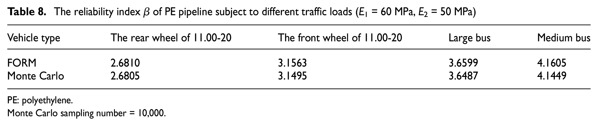
PE: polyethylene.

Monte Carlo sampling number = 10,000.

Figure 11.

The reliability index $β$ of PE pipeline versus material properties with the road surface.

It can be seen from Table 8 that under the different actions of vehicles, the reliability of PE pipeline also performs differently. The larger the vehicle load, the smaller is the value of reliability index. The reliability index of PE pipeline is about 3.15 under the action of 11.00-20 front wheel, 2.68 under the action of 11.00-20 rear wheel, 3.65 under the action of large bus, and 4.15 under the action of medium bus. With the decline of pavement performance, the reliability index of the pipeline shows a sharply downward trend in Figure 11. In other words, the reliability decreases accordingly.

It is assumed that the degradation curve of road performance is shown in the green curve in Figure 12. The life of PE pipeline can be obtained by combining the degradation curve of road performance (E–n curve) and the changing curve of PE pipeline reliability with road performance (r–E curve). For example, when the target reliability index of PE pipeline is r_limit, the pavement performance E_limt can be obtained from the r–E curve. Then, the limit service life n_limit can be obtained from the E–n curve. In addition, when service time n of PE pipeline is known, the corresponding residual life of PE pipeline is n_limit– n years.

Figure 12.

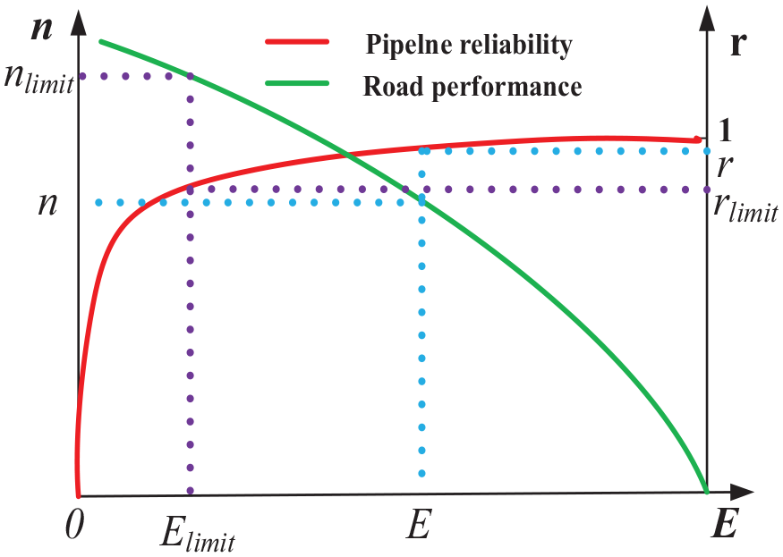
Life prediction diagram of PE pipeline.

Conclusion

In this article, pipeline mechanical model is established and a simple analysis carried out. Stress and stress distribution of pipeline are calculated by single random variables of traffic load. According to von Mises yield criterion, the limit state equation is set up. The reliability index of PE pipeline which under the action of traffic was calculated using central point method and Monte Carlo method.

After the actual tensile test, the yield strength of PE pipeline material at the tensile rate of 50 mm/min is generally in accordance with the normal distribution of N∼ (21.13, 2.172).

The maximum equivalent stress of the PE pipeline increases along with the raise of traffic loads and the aging of pavement materials. There is an exponential relationship between stress and traffic loads.

The limit state equation of buried PE pipeline under traffic load is established, and the reliability index of pipeline is calculated using the central point method and Monte Carlo method. The larger the vehicle load, the smaller is the value of reliability index. With the decline of pavement performance, the reliability index of the pipeline shows a sharply downward trend.

Based on the studies about the aging performance of pavement materials, the remaining service life of the PE pipeline, under a certain target reliability index, can be calculated, which provides a new prospect for the life assessment of PE pipeline crossing the road.

The stress environment of the buried PE pipeline under traffic load is simplified in the current work, considering the more independent random variables. Future work should focus on forming an entire pipeline life assessment method through a comprehensive analysis of these factors: the aging of actual pavement materials, the number of vehicles, and the reliability of pipelines.

Footnotes

Appendix 1 Acknowledgements

This work was supported by the China Scholarship Council and Science & Technology Program of Sichuan Province, China (No.2019YFS0075).

Handling Editor: Vesna Spasojevic Brkic

Declaration of conflicting interests

The author(s) declared no potential conflicts of interest with respect to the research, authorship, and/or publication of this article.

Funding

The author(s) received the following financial support for the research, authorship, and/or publication of this article: This project was supported by the China Scholarship Council and Science & Technology Program of Sichuan Province, China (No.2019YFS0075).

ORCID iDs

Wu Ying

Zha Si Xi

References

Luo

Zheng

, et al. Finite element analysis of buried polyethylene pipe subjected to seismic landslide. J Press Vess 2014; 136: 031801.

Ying

Sixi

Pengwei

Finite element method simulations to study factors affecting buried pipeline subjected to debris flow. J Press Vess 2019; 141: 021701.

Luo

Shi

, et al. Numerical simulation of strength failure of buried polyethylene pipe under foundation settlement. Eng Fail Anal 2015; 48: 144–152.

Cao

Han

, et al. Road surface permanent deformations with a shallowly buried steel-reinforced high-density polyethylene pipe under cyclic loading. Geotext Geomembranes 2016; 44: 28–38.

Zhang

Branam

Zand

, et al. A new approach to determine the stresses in buried pipes under surface loading. In: Proceedings of the ASME international pipeline conference, volume 2: pipeline safety management systems; project management, design, construction and environmental issues; strain based design; risk and reliability; northern offshore and production pipelines, Calgary, AB, Canada, 26–30 September 2016. New York: American Society of Mechanical Engineers.

Wang

Zhong

Long

, et al. Study on dynamic strain regularity and influencing factors of shallow buried metal pipe under collapse impact load. Shock Vib 2018; 2018: 8792564.

Alzabeebee

Chapman

Faramarzi

Economical design of buried concrete pipes subjected to UK standard traffic loading. P I Civil Eng: Str B 2019; 172: 141–156.

Kang

Parker

Yoo

CH.

Soil-structure interaction and imperfect trench installations for deeply buried concrete pipes. J Geotech Geoenviron 2007; 133: 277–285.

Alzabeebee

Chapman

Jefferson

, et al. The response of buried pipes to UK standard traffic loading. Geotech Eng 2017; 170: 38–50.

10.

Ban

Park

S-W

Kim

Y-R.

Performance evaluation of buried concrete pipe under heavy traffic load. J Korean Geotech Soc 2013; 29: 69–75.

11.

Chou

Wittenberg

Adeeb

, et al. Buried steel pipeline design: external load methodologies and strain limits. In: Proceedings of the international pipeline conference, Calgary, AB, Canada, 29 September–3 October 2014. New York: American Society of Mechanical Engineers.

12.

Wang

Sun

Zhang

, et al. Mechanical behaviors of the thin-walled SHCC pipes under compression. In: Proceedings of the 2015 international conference on transportation information & safety, Wuhan, China, 25–28 June 2015, pp.797–798. New York: IEEE.

13.

Fang

Wang

, et al. The mechanical behaviour of drainage pipeline under traffic load before and after polymer grouting trenchless repairing. Tunn Undergr Sp Tech 2018; 74: 185–194.

14.

Wang

, et al. Full-scale experimental study of the dynamic performance of buried drainage pipes under polymer grouting trenchless rehabilitation. Ocean Eng 2019; 181: 121–133.

15.

Rakitin

. Full-scale field test of large diameter reinforced concrete pipes under heavy traffic loads. In: Proceedings of the 5th international young geotechnical engineers conference, Paris, 31 August–1 September 2013, pp.353–356. Delft:Delft University Press.

16.

Arockiasamy

Chaallal

Limpeteeprakarn

Full-scale field tests on flexible pipes under live load application. J Perform Constr Fac 2006; 20: 21–27.

17.

Rakitin

Centrifuge testing to simulate buried reinforced concrete pipe joints subjected to traffic loading. Can Geotech J 2015; 52: 1762–1774.

18.

Meesawasd

Boonyasiriwat

Kongnuan

, et al. Finite element modeling for stress analysis of a buried pipeline under soil and traffic loads. In: Proceedings of the 2016 IEEE international conference on industrial engineering & engineering management, Bali, Indonesia, 4–7 December 2016. New York: IEEE.

19.

Khademi-Zahedi

Alimouri

Finite element analysis to the effect of thermo-mechanical loads on stress distribution in buried polyethylene gas pipes jointed by electrofusion sockets, repaired by PE patches. Energies 2018; 11: 2818.

20.

Fang

, et al. Numerical simulation and full-scale test on dynamic response of corroded concrete pipelines under multi-field coupling. Constr Build Mater 2019; 200: 368–386.

21.

Zhou

Nessim

Rothwell

, et al. Development of reliability-based design and assessment standards for onshore natural gas transmission pipelines. J Press Vess 2006; 131: 965–972.

22.

Teixeira

Soares

Netto

, et al. Reliability of pipelines with corrosion defects. Int J Pres Ves Pip 2008; 85: 228–237.

23.

Zhou

System reliability of corroding pipelines. Int J Pres Ves Pip 2010; 87: 587–595.

24.

Lee

Kim

Choi

SS.

Reliability of buried pipeline using a theory of probability of failure. Solid State Phenom 2006; 110: 221–230.

25.

Alimi

Chaoui

Amirat

, et al. Study of reliability index for high-density polyethylene based on pipe standard dimension ratio and fracture toughness limits. Int J Adv Manuf Tech 2018; 96: 123–136.

26.

Yun

Kang

Reliability analysis of high pressure buried pipeline under landslide. Appl Mech Mater 2014; 501–504: 1081–1086.

27.

Zhou

Reliability of pressurised pipelines subjected to longitudinal ground movement. Struct Infrastruct Eng 2012; 8: 1123–1135.

28.

Tee

Khan

HS.

Reliability analysis of underground pipelines using subset simulation. Int J Civil Environ Struct Constr Archit Eng 2013; 7: 843–849.

29.

Zhang

Song

, et al. Method on damage probability of pipelines under random traffic loads. Water Resour Hydropower Eng 2004; 35(10): 64–66. (in Chinese)

30.

Zhang

, et al. Reliability analysis method for remaining life of pipelines under traffic loads based on damage cumulative model. Water Resour Hydropower Eng 2004; 35(2): 66-67. (in Chinese)

31.

GB/T8804.3:2003. Thermoplastic pipes—determination of tensile properties—part 3: polyolefin pipes.

32.

Suleiman

Coree

BJ.

Constitutive model for high density polyethylene material: systematic approach. J Mater Civil Eng 2004; 16: 511–515.

33.

Gou

WJ.

Study on mechanical characteristics of buried pipelines under the roadway. Master’s Thesis, Chongqing University, Chongqing, China, 2016. (in Chinese)

34.

Liao

Huang

XM.

Application of ABAQUS finite element software in road engineering. Nanjing, China: Southeast University Press, 2008. (in Chinese)

35.

Hill

On discontinuous plastic states, with special reference to localized necking in thin sheets. J Mech Phys Solids 1952; 1: 19–30.

36.

CJJ63:2008. Technical specifications for polyethylene (PE) fuel gas pipeline engineering.

37.

GB50028:2006. Code for design of city gas engineering.

38.

Yuan

Guo

Pei

, et al. Truck load probabilistic characteristics of G104 highway. J Beijing Univ Tech 2017; 43: 1697–1705. (in Chinese)

39.

Wang

Chang

PM.

Analysis of tire inflating pressure of road transport vehicle. Tire Ind 2008; 3: 131–134. (in Chinese)

40.

Kapur

KC.

Reliability bounds in probabilistic design. IEEE T Reliab 1975; R–24: 193–195.

Reliability analysis of buried polyethylene pipeline subject to traffic loads

Abstract

Keywords

Introduction

Uniaxial tensile test

Calculation of maximum pipeline stress under traffic load

Conditional hypothesis

Material parameters

Model establishment

Numerical calculation

Calculation of pipeline reliability

Distribution law of vehicle loads

Yield strength distribution

Reliability calculation

Conclusion

Footnotes

Appendix 1

Acknowledgements

Declaration of conflicting interests

Funding

ORCID iDs

References