Sage Journals: Discover world-class research

Abstract

Bolted joints are elements used to create resistant assemblies in the mechanical system, whose overall performance is greatly affected by joints’ contact stiffness. Most of the researches on contact stiffness are based on certainty theory whereas in real applications the uncertainty characterizes the parameters such as fractal dimension D and fractal roughness parameter G. This article presents an interval estimation theory to obtain the stiffness of bolted joints affected by uncertain parameters. Topography of the contact surface is fractal featured and determined by fractal parameters. Joint stiffness model is built based on the fractal geometry theory and contact mechanics. Topography of the contact surface of bolted joints is measured to obtain the interval of uncertain fractal parameters. Equations with interval parameters are solved to acquire the interval of contact stiffness using the Chebyshev interval method. The relationship between the interval of contact stiffness and the uncertain parameters, that is, fractal dimension D, fractal roughness parameter G, and normal pressure, can be obtained. The presented model can be used to estimate the interval of stiffness for bolted joints in the mechanical systems. The results can provide theoretical reference for the reliability design of bolted joints.

Keywords

Bolted joint fractal theory Chebyshev interval method stiffness estimation uncertain parameters

Introduction

Accounting for up to 50% of the total stiffness of the mechanical system, the stiffness of bolted joint can affect the overall performance of systems.¹ Some models of bolted joint based on the certainty theory have been presented to study the characteristics of joints.^2–4 However, uncertainty exists in parameters such as the fractal dimension, fractal roughness parameters, and bolt pre-tightening force. Machining error and measurements make fractal dimension and fractal roughness uncertain. The certainty theory may result in a bigger error when the number of uncertain parameters is raised or the uncertainty range increased. Therefore, establishing a consistent theoretical background and modeling is necessary for predicting the stiffness of the bolted joints accurately.

Fractal contact theory has been widely applied to the analysis of the joint surface problems for the self-similarity and self-affinity of machined surfaces. A Majumdar and CL Tien⁵ gave a fractal representation of the roughness surface using the Weierstrass–Mandelbrot (W-M) function⁶ which defined a roughness surface through fractal parameters, that is, fractal dimension D and fractal roughness parameter G. A Majumdar and B Bhushan⁷ first presented a fractal contact model (Majumdar–Bhushan (M-B) model) of elastic and plastic contact of rough surface with scale independence. Through the model, the total real contact area and the normal load based on the two-dimensional W-M function and Hertz theory are calculated. Further research, based on the Hertz contact theory and capacity dissipation theory, improved this method for calculating the contact stiffness and damping. S Wang and K Komvopoulos⁸ presented an improved size-distribution function of the micro-contact spot with a domain extension factor ψ and divided the contact deformation of the asperity into three stages, that is, the totally elastic stage, the elastic–plastic stage, and the totally plastic stage. W Yan and K Komvopoulos⁹ presented a more accurate model about the contact of the three-dimensional anisotropic fractal surface for calculating the real contact area and the total normal load. In addition, the stiffness of the bolted joint can be obtained by testing of static loading deformation,¹⁰ and Daisuke et al.¹¹ introduced this method to approximately solve the contact stiffness by the fitting method. They applied the stiffness parameter to finite element model (FEM) analysis of a machine tool, in which the results show that the FEM with the contact stiffness is considered to be closed for the machine–foundation interface. You and Chen¹² presented that the simulation of the joint surface with the detailed division is closer to the practical surface. Zhao et al.¹³ presented a nonlinear virtual material method based on surface contact stress to describe the bolted joint for accurate dynamic performance analysis of the bolted assembly. R Grzejda¹⁴ put forward a thesis that modeling dissymmetric nonlinear multi-bolted connections as a system is possible. The model which can be applied to determine the changes in bolt forces, as well as in the normal contact pressure between the joined elements during the tightening of the system and at its end, was presented. In the traditional stiffness model based on fractal contact theory, the researchers assumed that the fractal dimension, fractal roughness parameters, and bolt pre-tightening force are considered as the certainty parameters. Actually, many uncertainties are inherent in loads, geometry, and manufacturing tolerance.

In recent years, more and more attention has been paid to the uncertainty of engineering problem.^15,16 Many uncertain parameters such as external load, material characteristics, and machining error in the actual bolted joint exist. All these external uncertainties can vary micro-fractal parameters, and the uncertain parameters lead to the change of system’s characteristics.¹⁷ Bifurcation will takes place in nonlinear systems even the effect parameters small and slow variation, thus the uncertainty of stiffness of bolted joints needs to be investigated.

The numerical algorithm of the uncertainty problem mainly contains the probability method, the fuzzy algorithm, and the interval algorithm. Probability algorithm has been widely used to deal with many uncertainty problems.^18,19 The probability method assumes that the distribution information of uncertain parameters is known; however, in practical problems, the distribution function of the parameters is difficult to obtain and the application of the method is thus limited. Fuzzy algorithm²⁰ is another kind of uncertainty analysis method that studies the phenomenon of uncertainty arising from the fuzziness of the concept, using the membership degree to describe the nature of this kind of uncertainty. Fuzzy mathematics is mainly used in pattern recognition, clustering analysis, comprehensive evaluation, mathematical logic, and decision-making. Recently, the fuzzy theory has been used to solve the fuzzy differential equations.^21,22

Interval method based on the set theory belongs to the non-probabilistic methods. In recent years, this method has drawn much attention in the field of uncertainty analysis and design.^23,24 Interval variables are used to represent upper and lower bounds of the uncertain-but-bounded parameters. The interval model makes it possible to measure uncertainties for bounded parameters being the complete information of the system unknown. The determination of lower and upper bounds for uncertain parameters is much easier than the identification of a precise probability distribution. However, the main shortcoming of this method is the relatively overestimation caused by the wrapping effect.²⁵ Therefore, how to effectively control the overestimation is the key to the interval arithmetic. Several interval methods have been applied to solve wrapping effect;^26,27 interval Taylor series and Taylor model^28,29 methods are the two typical methods. This method uses the high-order Taylor series expansion to approximate the true solution, but it is limited to the problem with a lower level of uncertainties. Compared with the Taylor method, the Chebyshev series method³⁰ can approximate the true solution, through which higher numerical accuracy can be achieved. Moreover, the Chebyshev inclusion function can effectively control the overestimation effect.

Studies of bolted joints concerning the uncertainty are still only a few. M Hanss et al.³¹ considered the eigenfrequency and the damping ratio as fuzzy numbers and used the transformation method to get the uncertain stiffness and damping. QT Guo and LM Zhang³² implied that joint parameters of some structures have normal or nearly normal distributions, and linear FEM with probabilistic variable could illustrate the dynamic characteristics of joints. N Norrick³³ focuses on the bolted joints between the main drive train gears and cylinders and shows how the statistical consideration of uncertainties enables us to design these joints. A failure probability for a specific gear-cylinder connection is calculated by considering statistical information gained from experimental data and using the Monte Carlo method. In the study by D Jiang et al.,³⁴ based on the theory of thin layer element, a parameter identification method for the uncertainty of bolted contact surface is proposed. The uncertainty FEM correction theory–based perturbation is used to identify the contact surface parameters. Seibel et al.³⁵ introduced closed-form symbolic expressions for the possibility distributions of the coefficients of friction during the tightening process of bolted joints. This relieves the engineer from the burden of propagating the uncertainties through the computations to obtain the uncertain output. N Imamovic and M Hanafi³⁶ investigated the uncertainty quantification of bolted joint beams, and the frequency response functions (FRFs) were measured in high-frequency range for all beams under varying conditions of torque applied to bolts in the structural joints. Roughness of surfaces that are in contact at structural joints is measured and considered as a source of uncertainty, with a discussion of characterization of bolted joint as a deterministic or stochastic model. The model is validated by comparing predicted and measured FRFs. However, these studies only focused on the uncertainty of macroscopic stiffness and damping and could not establish the relationship between microscopic uncertainty and macroscopic characteristic of the bolted joints.

This article combines the fractal theory and the Chebyshev interval method to estimate the contact stiffness of bolted joint with uncertain parameters. The fractal dimension and fractal roughness parameter are considered as the uncertain parameters. These fractal uncertain characteristic parameters are determined by the power spectrum method. Interval models of uncertain parameters are introduced to the fractal model and the equations are solved through the Chebyshev interval method. Normal and tangential stiffness are calculated based on the fractal model in microscale, whereas the upper and lower boundaries of the normal and tangential stiffness are determined through the Chebyshev interval method. The relationship between stiffness interval, fractal dimension, fractal roughness parameter, and the normal pressure can be obtained. The presented method can be used to determine the upper and lower boundaries of the stiffness affected by uncertain parameters. The result can provide a theoretical basis for improving the reliability of the systems with bolted joints.

Mechanism of the three-dimensional fractal contact model

Fractal theory is used to describe the geometric features of contact surfaces, which provides a method of describing asperities with a wide range of size. The fractal rough surface profile is expressed by W-M function

\begin{array}{l} z (x) = L {(\frac{G}{L})}^{(D - 1)} {(\ln γ)}^{1 / 2} \sum_{n = 0}^{n_{\max}} γ^{(D - 2) n} \\ [\cos ϕ_{1 n} - \cos (\frac{2 π γ^{n} x}{L} - ϕ_{1 n})] \end{array}

(1)

where z is the surface height, x denotes the transverse distance, L is the length of a fractal sample, G is the fractal roughness parameter, D is the fractal dimension (1 < D < 2), γ = 1.5 is the scaling parameter, and ϕ_1n is the random phase.

It is assumed that the rough surfaces are isotropic, and the fractal dimension D and roughness parameter G remain unchanged during the contact process. For microscale, the asperities of two rough surfaces are actually squeezed each other, as shown in Figure 1. The two rough surfaces in contact can be simplified as a rigid smooth surface and an equivalent rough surface. The equivalent roughness surface is characterized by an equivalent elastic.

Figure 1.

Contact deformation of the single micro-convex body.

The contact surface is formed of micro-convex bodies whose deformation is divided into elastic deformation and plastic deformation stages. The deformation stage is determined from critical deformation and critical cross-sectional area. For a single micro-convex body, the radius of curvature of R and normal deformation can be expressed by combining the surface fractal parameters, that is, fractal dimension D and surface roughness parameter G

R = \frac{a^{(D - 1) / 2}}{2^{5 - D} π^{(D - 1) / 2} G^{D - 2} {(\ln γ)}^{1 / 2}}

(2)

δ = 2 G^{D - 2} {(\ln γ)}^{\frac{1}{2}} {(2 r)}^{3 - D}

(3)

where a is the cross-sectional area of a single micro-convex body; r is the cross-sectional area of the micro-convex body, $r^{2} = 2 R δ (R >> r)$ ; γ is the scale parameter.

The critical deformation δ_c and the critical truncated area a_c of the single asperity for demarcating the elastic and elastic–plastic regimes are given by

δ_{c} = {(\frac{π kH}{2 E})}^{2} R

(4)

a_{c} = {[\frac{2^{11 - 2 D} G^{2 (D - 2)} (\ln γ) E^{2}}{π^{4 - D} {(kH)}^{2}}]}^{\frac{1}{D - 2}}

(5)

where H is the hardness of the soft material which can be obtained from the relationship with yield stress Y as H = 2.8Y; ν₁, ν₂, E₁, and E₂ are the Poisson ratio and elastic modulus of two contacting surfaces, respectively, and k = 0.454 + 0.41ν is the coefficient related with the Poisson ratio.

The three-dimensional size-distribution function can be written as

n (a) = \frac{D - 1}{2} {a_{l}}^{(D - 1) / 2} a^{(- D - 1) / 2}

(6)

Total real contact area and load

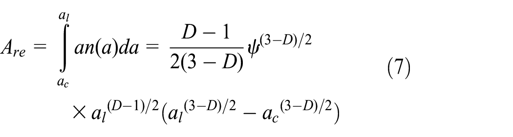
According to the fractal theory, when a_c < a < a_l, the contact surface micro-convex bodies are in the elastic deformation stage, and the total real elastic contact area A_re can be obtained by integrating the distribution function of micro-convex cross-sectional area in the elastic deformation area

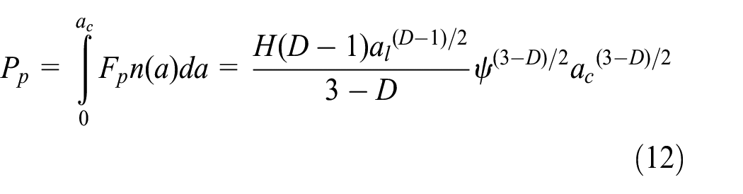
\begin{matrix} A_{re} = \int_{a_{c}}^{a_{l}} an (a) da = \frac{D - 1}{2 (3 - D)} ψ^{(3 - D) / 2} \\ \times {a_{l}}^{(D - 1) / 2} ({a_{l}}^{(3 - D) / 2} - {a_{c}}^{(3 - D) / 2}) \end{matrix}

(7)

When 0 < a < a_c, the contact surface micro-convex bodies are in the plastic deformation stage, and the total real plastic contact area A_rp can be obtained by integrating the distribution function of micro-convex cross-sectional area in the plastic deformation area

A_{rp} = \int_{0}^{a_{c}} an (a) da = \frac{D - 1}{3 - D} ψ^{(3 - D) / 2} {a_{l}}^{(D - 1) / 2} {a_{c}}^{(3 - D) / 2}

(8)

According to the above equations, the total real contact area is

A_{r} = {\begin{matrix} A_{re} + A_{rp} a_{l} > a_{c} \\ A_{rp} 0 < a_{l} < a_{c} \end{matrix}

(9)

The normal load of the joint surface is the connection point between macroscopic mechanical properties and microscopic fractal theory model. The three-dimensional fractal theory and the micro-convex body size-distribution function are combined to establish the total normal load of the elastic and plastic deformation stage.

The elastic and plastic loads of a single micro-convex body are obtained based on the Hertz theory

F_{e} = \frac{4 E r^{3}}{3 R}, F_{p} = Ha

(10)

where F_e is the elastic load and F_p is the plastic load of a micro-convex body.

The total elastic contact load and plastic contact load of the joint surface can be expressed as

\begin{matrix} P_{e} = \int_{a_{c}}^{a_{l}} F_{e} n (a) da \\ = {\begin{matrix} \frac{2^{(11 - 2 D) / 2}}{3 π^{(4 - D) / 2}} \cdot \frac{D - 1}{5 - 2 D} ψ^{(3 - D) / 2} (\ln γ)^{1 / 2} G^{(V - 2)} E {a_{l}}^{(D - 1) / 2} \\ ({a_{l}}^{(5 - 2 D) / 2} - {a_{c}}^{(5 - 2 D) / 2}) (D \neq 2.5) \\ 2 π^{- 3 / 4} ψ^{(3 - D) / 2} (\ln γ)^{1 / 2} G^{1 / 2} E {a_{l}}^{3 / 4} \ln (\frac{a_{l}}{a_{c}}) (D = 2.5) \end{matrix} \end{matrix}

(11)

P_{p} = \int_{0}^{a_{c}} F_{p} n (a) da = \frac{H (D - 1) {a_{l}}^{(D - 1) / 2}}{3 - D} ψ^{(3 - D) / 2} {a_{c}}^{(3 - D) / 2}

(12)

Then the total normal load P is

P = {\begin{matrix} P_{e} + P_{p} a_{l} > a_{c} \\ P_{p} 0 < a_{l} < a_{c} \end{matrix}

(13)

Assuming the pressure distribution is uniform, the equivalent pressure of joint surface can be expressed as

\bar{P} = \frac{P}{A_{a}}

(14)

Normal and tangential stiffness model of joint surface

Normal stiffness of joint surface

Based on the Hertz theory, the normal stiffness of a single micro-convex body can be expressed as

k_{n} = \frac{d F_{e}}{d δ}

(15)

The normal stiffness of joint surface can be obtained by integrating k_n in the elastic deformation region

\begin{matrix} K_{ne} = \int_{a_{c}}^{a_{l}} k_{n} n (a) da = \frac{2 \sqrt{2} E (4 - D) (D - 1)}{3 \sqrt{π} (3 - D) (2 - D)} \\ \times {a_{l}}^{(D - 1) / 2} ({a_{l}}^{(2 - D) / 2} - {a_{c}}^{(2 - D) / 2}) \end{matrix}

(16)

When the stiffness of plastic deformation is zero, the total stiffness model is described as

K_{n} = {\begin{matrix} K_{ne} a_{l} > a_{c} \\ 0 0 < a_{l} < a_{c} \end{matrix}

(17)

Tangential stiffness of joint surface

According to the former research,⁹ the tangential deformation of a single micro-convex body can be written as

δ_{t} = \frac{3 μ p}{16 G' r} [1 - {(1 - \frac{t}{μ p})}^{2 / 3}]

(18)

where p is the normal load of the single convex body; when the micro-convex body is in the elastic deformation stage, p = F_e; when the micro-convex body is in the plastic deformation stage, p = F_p; t is the tangential load of a single convex body, G′ is the equivalent shear modulus of the contacting material, 1/G′ = (2 – ν₁)/G₁ + (2 – ν₂)/G₂. μ is the contact surface friction factor and r is the radius of real contact area.

The tangential stiffness of single convex body can be expressed as k_t = dt/dδ_t, and the tangential stiffness can be obtained by the integration of k_t in the elastic deformation region

\begin{matrix} K_{te} = \int_{a_{c}}^{a_{l}} k_{t} n (a) da = \frac{8 G' (D - 1) ψ^{(3 - D) / 2}}{\sqrt{2 π} (2 - D)} \\ \times {(1 - \frac{t}{μ p})}^{1 / 3} {a_{l}}^{(D - 1) / 2} ({a_{l}}^{(2 - D) / 2} - {a_{c}}^{(2 - D) / 2}) \end{matrix}

(19)

The ratio of normal load and tangential load to a single micro-convex body t/p = T/P is satisfied, where T is total tangential stiffness of joint surface and T = τ_bA_r; τ_b is the shear strength of soft material.

To sum up, the total tangential stiffness of joint surface K_t can be expressed as follows

K_{t} = {\begin{matrix} K_{te} a_{l} > a_{c} \\ 0 0 < a_{l} < a_{c} \end{matrix}

(20)

Uncertainty parameters of the bolted joints

In traditional fractal contact theory, the researchers assume the fractal dimension, fractal roughness parameter, and bolt pre-tightening force as certain parameters. However, all of these parameters are uncertain due to machining error, finishing, measurements, and external load. In this section, the fractal uncertainty parameters will be discussed and determined by experimental measurements and the power spectrum method.

The uncertain parameters D and G

Based on the derivation above (section “Mechanism of the three-dimensional fractal contact model”), the fractal dimension D and surface roughness parameter G significantly affect the stiffness of bolted joints. Most of the scholars studied the characteristics of a joint surface based on the certainty theory, where D and G are considered to be determined values. However, D and G are uncertain due to the above reasons so, in this section, the uncertainty of D and G is quantified.

To obtain the uncertainty of parameters D and G, three specimens were taken as an example and measured, and all the values of roughness are 1.6 when they are finished. The specimens were machined and treated according to these three methods: milling only, grinding only, and heat-treatment grinding . Each surface was measured at three different locations, as shown in Figure 2. And the two-dimensional surface profile of the three specimens which processed with different processing methods is shown in Figure 3. Based on the power spectrum density method, the fractal dimension and fractal roughness parameter of contact surface can be obtained for each sample. The power spectrum of the contact surface is shown in Figure 4.

Figure 2.

Sample and measuring positions.

Figure 3.

The surface profile.

Figure 4.

The power spectrum of the contact surface.

Based on the power spectrum density method, the fractal dimension and fractal roughness parameter of contact surface are obtained, and their values are listed in Table 1. Different processing techniques lead to different values of the parameters, even though roughness was set to the same value before processing.

Table 1.

Parameters’ value of the contact surface processed by different methods.

	Ra(1.6)	D	G
Milling	1.6078	1.1594	3.1683e–17
Grinding	1.1857	1.1478	6.9200e–17
Heat-treatmentgrinding	1.1376	1.1497	1.5529e–17
Mean value	1.3104	1.1523	3.8804e–17
Variance ratio	0.226	0.006	0.783

The variation ratio of D is 0.6%, big enough to be regarded as an interval containing all the possible values instead of considering it as a determined value. Fractal roughness parameter G changes in a rather big field with a variation ratio of 78.3%, which means that regarding it as a certain number can lead to big errors in the estimation of contact stiffness.

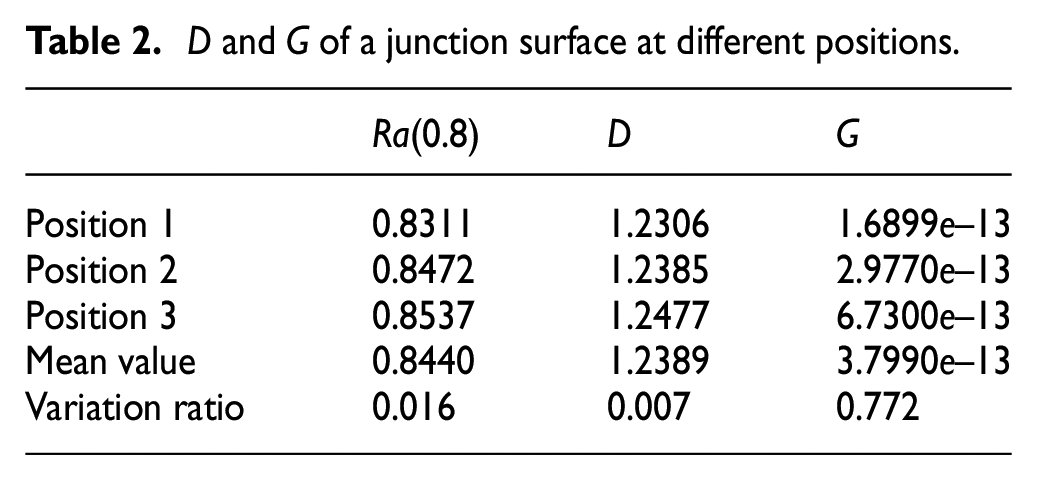
For the same junction surface whose roughness is 0.8, the surface profile (see Figure 2) was tested at different positions. Also, in this case, the parameters listed in Table 2 change within a certain range. From Table 2, it is observed that the variation ratio of D is 0.7%, and fractal roughness parameter G changes in a rather big field with a variation ratio of 77.2%, which means that regarding them as certain numbers can lead to big errors in the estimation of contact stiffness. Even if the measurements are taken at different locations for the same surface, the resulting D and G are not deterministic, and fluctuation ranges cannot be ignored.

Table 2.

D and G of a junction surface at different positions.

	Ra(0.8)	D	G
Position 1	0.8311	1.2306	1.6899e–13
Position 2	0.8472	1.2385	2.9770e–13
Position 3	0.8537	1.2477	6.7300e–13
Mean value	0.8440	1.2389	3.7990e–13
Variation ratio	0.016	0.007	0.772

Uncertainty of bolted joints using interval parameters

Due to the high number of uncertain parameters in bolted joints, traditional probabilistic models for the distribution information are not suitable to describe the uncertainty whereas the bound of the parameters can be easily obtained based on the above analysis. It proved that parameter uncertainties of bolted joints can be mathematically described through interval variables. Interval variables are used to represent upper and lower bounds of the uncertain-but-bounded parameters. In the fractal model of bolted joint, the upper and lower bounds of the uncertain parameters are obtained in the following.

The basic definitions of interval arithmetic

The uncertain parameter can be expressed by a real interval set $[x]$ containing all its possible values, and it is written as

[x] = [\underline{x}, \bar{x}] = {x \in R : \underline{x} \leq x \leq \bar{x}}

(21)

where $\underline{x}$ is the lower bound of $[x]$ representing the smallest number of all possible values; $\bar{x}$ is the upper bound of $[x]$ representing the biggest number of all possible values.

Define the midpoint of $[x]$ by

x_{c} = mid ([x]) = \frac{\bar{x} + \underline{x}}{2}

(22)

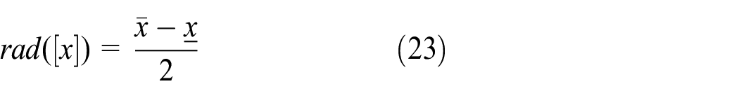
Define the radius of $[x]$ by

rad ([x]) = \frac{\bar{x} - \underline{x}}{2}

(23)

Express the width of $[x]$ as

w ([x]) = 2 \times rad ([x])

(24)

Therefore, the interval can also be written as

[x] = x_{c} + [Δ x]

(25)

Δ x = [- \frac{w ([x])}{2}, \frac{w ([x])}{2}]

(26)

where $Δ x$ is the symmetric interval of $[x]$ .

Interval arithmetic operation is defined on the real set R. Therefore, the four classic algorithms (add, subtract, multiply, and divide) also suit for the interval variables, so it is called interval algorithm. Taken two real intervals $[x]$ and $[y]$ as an example, the four arithmetic operations are

\begin{matrix} [x] * [y] = {x * y \in R : x \in [x], y \in [y]} \\ * \in {\pm, \times, \div} \end{matrix}

(27)

If there is a real function $f$ defined in the field of real numbers whose independent variable is the interval $[x]$ , the interval function $[f]$ of the real function $f$ is defined as

[f] ([x]) \supset f ([x])

(28)

The interval function $[f]$ of $f$ is called inclusion function. Only by the inclusion function $[f]$ , the interval analysis can be achieved, so the main goal is to find the proper inclusion function $[f]$ .

To this end, this article selects the Chebyshev inclusion function due to the characteristics of uncertain parameters in bolted joints, having Chebyshev higher numerical accuracy than other inclusion functions.

Chebyshev inclusion function

If function $f (x)$ is continuous in the interval $[a, b]$ , there must exist an polynomial p(x) which uniformly approximates to the function $f (x)$ in $[a, b]$ . This approximate relationship can be expressed as

‖ f (x) - p (x) ‖ \leq ε, x \in [a, b]

(29)

which states that every continuous function can be approximated by any order polynomials to obtain any precision.

Using p_k(x) to stand for a set of polynomials whose degree is not bigger than k, then

p_{k} (x) = a_{0} + a_{1} x + a_{2} x^{2} + \dots + a_{k} x^{k}, x \in [a, b]

(30)

where a₀, a₁,…, a_k can be any real number.

For every single nonnegative integer k, there must be a unique polynomial $p_{k}^{*} (x)$ in $p_{k} (x)$ which satisfies the following expression

‖ f (x) - p_{k} (x) ‖_{\infty} \geq ‖ f (x) - p_{k}^{*} (x) ‖_{\infty}, x \in [a, b]

(31)

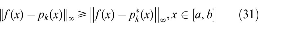
Equation (31) shows that $p_{k}^{*} (x)$ approximates $f (x)$ better than any other polynomials. However, $p_{k}^{*} (x)$ is difficult to obtain because of the too high computational load when k > 2.

This article selects the truncated Chebyshev polynomial to get the best uniform approximation polynomial with lower order. Considering a one-dimensional problem first, the one-dimensional Chebyshev series of degree k in $x \in [- 1, 1]$ is given by the explicit formula

C_{k} (x) = \cos (k θ)

(32)

where $θ = \arccos (x) \in [0, π]$ and k is the nonnegative integer.

The Chebyshev polynomial can also be defined in $x \in [a, b]$ , but then

θ = \arccos (\frac{2 x - (b + a)}{b - a}) \in [0, π]

(33)

The Chebyshev polynomials are orthogonal in the interval $x \in [- 1, 1]$ over a weight function $ρ (x) = 1 / \sqrt{1 - x^{2}}$ . In particular

\int_{- 1}^{1} \frac{C_{k} (x) C_{p} (x)}{\sqrt{1 - x^{2}}} d x = \int_{0}^{π} \cos k θ \cos p θ d θ = {\begin{matrix} π, k = p = 0 \\ π / 2, k = p \neq 0 \\ 0, k \neq p \end{matrix}

(34)

Assume a function $f (x)$ defined in an interval $x \in [a, b]$ , it can be approximated by the truncated Chebyshev series

f (x) \approx p_{k} (x) = \frac{1}{2} f_{0} + \sum_{i = 0}^{k} f_{i} C_{i} (x)

(35)

where $f_{i}$ are the coefficients, k is the degree of the series, and $C_{i} (x)$ is the Chebyshev polynomials of degree i.

The error between the Chebyshev series and the original function can be given as

e_{k} (f) = | f (x) - p_{k} (x) | \leq \frac{2^{- k}}{(k + 1)!} ‖ f^{(k + 1)} ‖_{\infty}

(36)

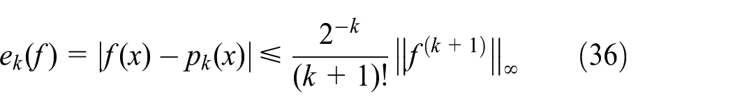
When k is big enough, the error can be neglected, meaning that high accuracy can be obtained.

The constant coefficients $f_{i}$ are the key to construct the Chebyshev series. Considering the integration of the original function $f (x)$ and $C_{p} (x)$ over the weight function $ρ (x)$

\begin{array}{l} \int_{- 1}^{1} \frac{1}{\sqrt{1 - x^{2}}} f (x) C_{p} (x) d x \approx \int_{- 1}^{1} \frac{1}{\sqrt{1 - x^{2}}} (\frac{1}{2} f_{0} + \sum_{i = 1}^{k} f_{i} C_{i} (x)) \\ C_{p} (x) d x \\ = \int_{- 1}^{1} \frac{1}{\sqrt{1 - x^{2}}} \frac{1}{2} f_{0} C_{p} (x) d x + \sum_{i = 1}^{k} \int_{- 1}^{1} \frac{1}{\sqrt{1 - x^{2}}} f_{i} C_{i} (x) C_{p} (x) d x \end{array}

(37)

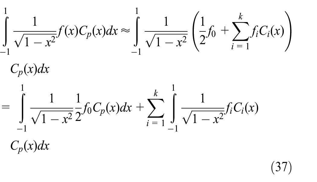
Considering the orthogonality of the Chebyshev series with respect to the weighting function, only when i = p ≠ 0

\int_{- 1}^{1} \frac{1}{\sqrt{1 - x^{2}}} C_{p} (x) \sum_{i = 1}^{k} f_{i} C_{i} (x) dx = \frac{π}{2} f_{p}

(38)

It is obtained that

\begin{matrix} \int_{- 1}^{1} \frac{1}{\sqrt{1 - x^{2}}} f (x) C_{p} (x) dx \approx \frac{π}{2} f_{p} \\ f_{p} = \frac{2}{π} \int_{- 1}^{1} \frac{1}{\sqrt{1 - x^{2}}} f (x) C_{p} (x) dx \end{matrix}

(39)

That is

f_{i} = \frac{2}{π} \int_{- 1}^{1} \frac{1}{\sqrt{1 - x^{2}}} f (x) C_{i} (x) dx = \frac{2}{π} \int_{0}^{π} f (\cos θ) \cos i θ d θ

(40)

where i = 1, 2,…, k.

The upper integral can be calculated by the interpolation integral method. The interpolation quadrature can be expressed as

\int_{a}^{b} ρ (x) f (x) dx = \sum_{j = 1}^{m} A_{j} f (x_{j})

(41)

where ρ(x) is the weighting function, x_j are the interpolation points, A_j are the integral coefficients, and m is the number of the interpolation points.

If the weighting function is ρ(x) = 1/(1 – x²)^1/2, the corresponding orthogonal polynomials are the Chebyshev polynomials. Then the interpolation points are the zeros of the Chebyshev polynomials of degree m given by

x_{j} = \cos θ_{j}, θ_{j} = \frac{2 j - 1}{p} * \frac{π}{2}

(42)

where j = 1, 2,…, m.

In this situation, all the integral coefficients are A_j = π/p. Then the next expression can be obtained as follows

\int_{- 1}^{1} \frac{1}{\sqrt{1 - x^{2}}} f (x) dx = \frac{π}{p} \sum_{j = 1}^{p} f (\cos θ_{j})

(43)

Concerning equations (40) and (43), the following can be obtained

\begin{matrix} f_{i} = \frac{2}{π} \int_{- 1}^{1} \frac{f (x) C_{i} (x)}{\sqrt{1 - x^{2}}} dx \approx \frac{2}{π} \frac{π}{p} \sum_{j = 1}^{m} f (x_{j}) C_{i} (x_{j}) \\ = \frac{2}{p} \sum_{j = 1}^{m} f (\cos θ_{j}) \cos i θ_{j} \end{matrix}

(44)

Concerning equations (34), since the coefficient is solved, the approximate Chebyshev series p_k(x) can be obtained. Then the Chebyshev inclusion function is expressed as

\begin{matrix} f (x) \in [f_{c}] ([x]) = \frac{1}{2} f_{0} + \sum_{i = 1}^{k} f_{i} C_{i} (x) = \frac{1}{2} f_{0} \\ + \sum_{i = 1}^{k} f_{i} \cos i [θ] = \frac{1}{2} f_{0} + [- 1, 1] \sum_{i = 1}^{k} [f_{i}] \end{matrix}

(45)

where f(x) is the original function and [f_c]([x]) is the Chebyshev inclusion function.

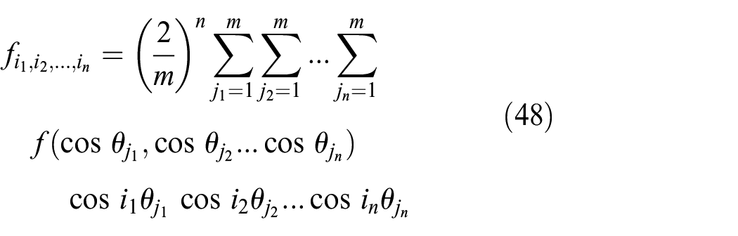
Now the multidimensional function is studied; assume a function f(x) defined in [–1, 1]ⁿ, then the Chebyshev polynomials are

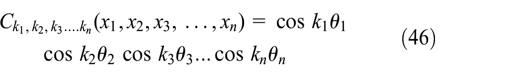
\begin{matrix} C_{k_{1}, k_{2}, k_{3} . . . . k_{n}} (x_{1}, x_{2}, x_{3}, \dots, x_{n}) = \cos k_{1} θ_{1} \\ \cos k_{2} θ_{2} \cos k_{3} θ_{3} . . . \cos k_{n} θ_{n} \end{matrix}

(46)

The approximate Chebyshev series can be expressed as

f (x) = \sum_{i_{1} = 0}^{k} {\sum_{i_{2} = 0}^{k} . . . \sum_{i_{n} = 0}^{k} (\frac{1}{2})}^{q} f_{i_{1}, i_{2}, \dots, i_{n}} C_{i_{1}, i_{2}, \dots, i_{n}} (x)

(47)

where n is the dimension of the problem, k is the order of the Chebyshev series, and q is the number of zeros between i₁, i₂,…, i_n. Concerning equation (43), the coefficients $f_{i_{1}, i_{2}, \dots, i_{n}}$ can be obtained by

\begin{matrix} f_{i_{1}, i_{2}, \dots, i_{n}} = {(\frac{2}{m})}^{n} \sum_{j_{1} = 1}^{m} \sum_{j_{2} = 1}^{m} . . . \sum_{j_{n} = 1}^{m} \\ f (\cos θ_{j_{1}}, \cos θ_{j_{2}} . . . \cos θ_{j_{n}}) \\ \cos i_{1} θ_{j_{1}} \cos i_{2} θ_{j_{2}} . . . \cos i_{n} θ_{j_{n}} \end{matrix}

(48)

The effect of interval parameters on the stiffness of bolted joints

Based on the analysis in Tables 1 and 3, the mean value of the uncertain parameter D is 1.2389, and the variation ratio is determined to be 0.005. According to equations (23)–(25), D can be written as

\begin{matrix} D_{c} = 1.2389 \\ rad [D] = 0.005 \times D_{c} = 6.1945 e - 3 \\ [D] = D_{c} + rad [D] \times δ = [1.2327, 1.2451] \end{matrix}

(49)

where $δ \in [- 1, 1]$ .

Table 3.

Values of parameters of the friction model.

Parameters	Value	Dimension
$γ$	1.5	–
$E_{1}, E_{2}$	2.1e11	Pa
$H$	1.96e9	Pa
$μ$	0.28	–
$P$	5e6	Pa

The mean value of uncertain parameter G is set to 3.7990e–13, and the variation ratio is set to 0.5. According to equations (23)–(25), G can be expressed as

\begin{matrix} G_{c} = 3.7990 e - 13 \\ rad [G] = 1.8995 e - 13 \\ [G] = G_{c} + rad [G] \times ξ = [1.8995 e - 13, 5.6985 e - 12] \end{matrix}

(50)

where $ξ = \in [- 1, 1]$ .

The bolted assembly is composed of two specimens and the pre-tightening force is provided by two M12 bolts. The material of specimens 1 and 2 is 45# steel with the roughness of 1.6 (Figure 5). For analyzing the characteristics of contact of bolted joints, the parameters’ values of $γ$ , E₁, E₂, H, μ, and P are listed in Table 3.

Figure 5.

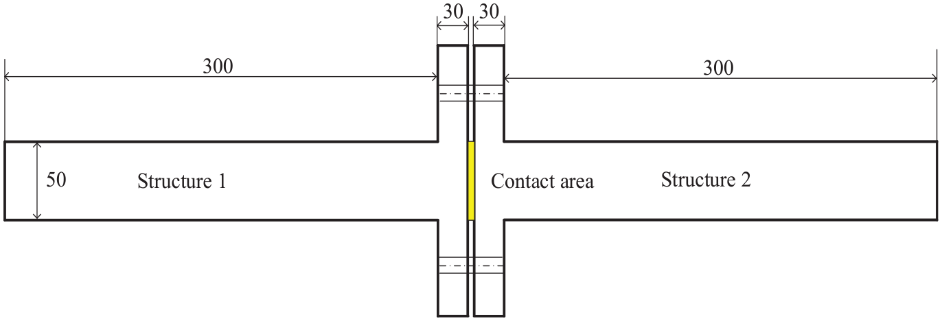
Schematic diagram of bolting structure.

Effects of D and G on A_c and A_l

According to equations (16) and (19), a_l and a_c influence the final total normal stiffness K_n and total tangential stiffness directly. Moreover, from equations (5), (10), and (11), the uncertain parameters D and G determine a_l and a_c, respectively. Therefore, the effects of D and G on a_l and a_c need to be discussed.

Effects of D and G on A_c

According to equation (5) and based on the Chebyshev interval method (equations (32)–(34) and (48)), a_c can be calculated by the interval number [D]; furthermore, [D] can be expressed by the non-dimensional angle θ. Therefore, a_c can finally be expressed by θ

θ = \arccos (δ) \in [0, π]

When $θ = 0, δ = \cos (θ) = 1, D = D_{c} + r a d [D] \times δ = 1.2327$ . When $θ = π, δ = \cos (θ) = - 1, D = D_{c} + r a d [D] \times δ = 1.2451$ .

The critical truncated area a_c of the joint surface increases with the increase of $θ$ from 0 to π (see Figure 6). In other words, a_c decreases with the increase of the uncertain parameter fractal dimension D from 1.2327 to 1.2451. The maximum value is a_c = 7.5376e–32 and the minimum value is a_c = 5.9684e–32. According to equations (21)–(24), a_c can be expressed as

\begin{matrix} [a_{c}] = [5.9684 e - 32, 7.5376 e - 32] \\ a_{cc} = (max a_{c} + min a_{c}) / 2 = 6.7530 e - 32 \\ rad [a_{c}] = (max a_{c} - min a_{c}) / 2 = 0.7846 e - 32 \end{matrix}

(51)

Figure 6.

The effect of D on $A_{c}$ .

It is concluded that the range ratio is 11.62%; compared with the range ratio 0.005 of D, even a slight change of D can lead to bigger fluctuations of a_c. This phenomenon often occurs in nonlinear problems.

Similarly, as it has been done for D, according to equations (5), (32)–(34), and (49), a_c can also be calculated by G, and it can finally be expressed by an angle α, where $α = \arccos (ξ) \in [0, π]$ .

In Figure 7, a_c decreases from 1.5106e–31 to 0.1678e–31 with the increase of α from 0 to π. Moreover, a_c increases with the increase of uncertain parameter G from 1.8995e–13 to 5.6958e–12. Like equation (50), it is obtained that [a_c] = [0.1678e–31, 1.5106e–31], a_cc=0.8392e–31, and rad[a_c]=0.6741e–31. The range ratio is 80% bigger than that of G of 0.5 and it cannot be neglected.

Figure 7.

The effect of G on $A_{c}$ .

In addition to the analysis of the effect of D and G on a_c separately, their comprehensive effects on a_c are analyzed to obtain the exact range interval of a_c. The two-dimensional and six-order Chebyshev interval methods were applied to this problem and the result is shown in Figure 8. The minimum value of a_c is 1.492e–32 and the maximum value of a_c is 1.6960e–31. Finally, it is obtained that [a_c] = [0.1492e–31, 1.6960e–31], a_cc = 0.9226e–31, rad[a_c] = 0.7734e–31, and the range ratio is 83.82%

Figure 8.

The effect of D and G on a_c.

Effect of D and G on A_l

Similar to the above analysis of the $A_{c}$ , according to equations (10)–(13), the effect of D and G on $A_{l}$ can be obtained by numerical approximation method. In this section, the Newton iteration and the Chebyshev interval method are combined to obtain the interval of $A_{l}$ . Moreover, the uncertain number (D, G) is represented by θ and α.

According to Figure 9, the interval varies with the iteration number and the order of the Chebyshev method; when the iteration number is bigger than 25, the interval tends to be constant and the interval iteration converges fast. When the order is bigger than 3, the interval tends to be constant too; thus, the order and iteration number are determined.

Figure 9.

The effect of order and iteration number on the interval.

When analyzing the effect of D, G is considered as a certain number. Finally, D and G are represented by θ and α, respectively, as shown in Figures 10 –12.

Figure 10.

The effect of D on $A_{l}$ .

Figure 11.

The effect of G on $A_{l}$ .

Figure 12.

The effect of D and G on $A_{l}$ .

The result of the above analysis on $A_{l}$ is summarized in Table 4. The interval of $A_{l}$ affected by D separately is [5.9088, 6.6476] and it is narrow compared with [4.2469, 7.1814] which affected by G separately. Furthermore, the comparison of variation ratios of 0.0588 and 0.2938 leads to a conclusion that the effect of G on $A_{l}$ is even greater than that of D. However, the effect of D and G at the same time needs to be considered to get the exact range interval. Choosing the two-dimensional Chebyshev interval method, the final interval is [3.9885, 8.2312]. The stiffness of the bolted joints is then computed using this final interval.

Table 4.

The result of the analysis about $A_{l}$ .

Influencefactor	Interval of $A_{l}$	Central value	Rad	Variationratio
D(E-10)	[5.9088, 6.6476]	6.2782	0.3694	0.0588
G(E-10)	[4.2469, 7.7814]	6.0142	1.7673	0.2938
D andG(E-10)	[3.9885, 8.2312]	6.1098	2.1213	0.3472

The effect of uncertain parameters on the stiffness of bolted joints

In section “Uncertainty parameters of the bolted joints,” the uncertain fractal parameters D and G were analyzed and the interval of D and G was calculated; in section “Effects of D and G on A_c and A_l,” the interval of A_l and A_c affected by uncertain parameters was obtained through the Chebyshev interval method. Concerning equations (16) and (19), K_n and K_t were determined by D, A_l, and A_c directly. In this section, the relationship between K_n, K_t and D, A_l, and A_c will be discussed.

Like the above analysis about D and G, A_l and A_c can also be expressed by the non-dimensional angle $θ$ and $α$ . Figure 13(a) shows that when the angle increases from 0 to π, which means the interval parameters decrease from the maximum value to the minimum value, K_n tends to decrease. Moreover, A_l greatly influences K_n whereas the impact of A_c is small because A_c is much smaller than A_l. Figure 13(b) shows the simultaneous effect of D and A_l on K_n; K_n reaches the maximum only when D and A_l assume the maximum value at the same time. The results are summarized in Table 5.

Figure 13.

The effect of D, A_l, A_c on $K_{n}$ : (a) separate effect of D, A_l, A_c on $K_{n}$ and (b) simultaneous effect of D and A_l on K_n.

Table 5.

The interval of $K_{n}$ effected by uncertain parameters.

Influence factor	Interval of K_n	Central value	Rad	Variation ratio
D	[7.1138, 7.6349]	7.3744	0.2485	0.0337
A_l	[5.9627, 8.5524]	7.2576	1.2949	0.1784
A_c	[7.3719, 7.3719]	7.3719	0	0
D-A_l-A_c	[5.7539, 8.8574]	7.3057	1.5518	0.2124

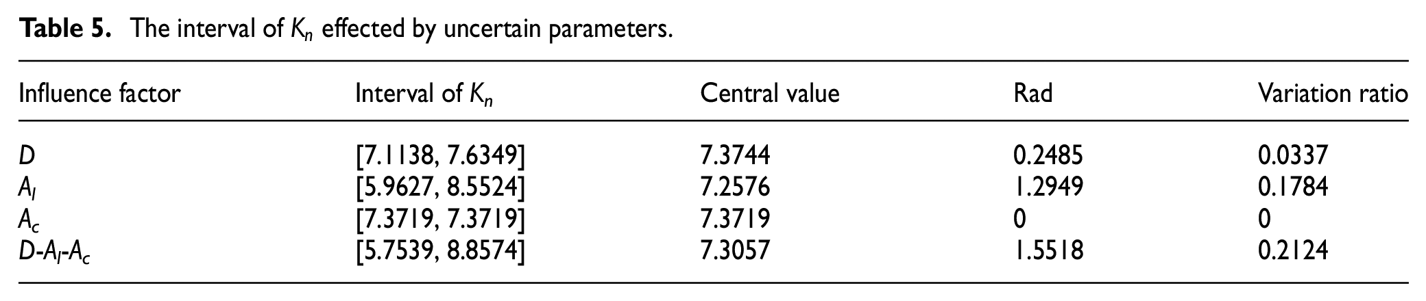
The normal stiffness calculated by the certain method is K_n = 7.433e5 and it is included in the interval. From Table 5, a variation ratio up to 0.2124 is big enough to change the dynamic behavior of bolted joints. In the design, manufacturing, and assembly processes, the variation ratio must be considered to enhance reliability and reduce the system failure probability.

Figure 14(a) shows the relationship between the normal pressure and normal stiffness. The normal stiffness tends to increase with the increase of normal pressure because of the increase of total real contact area A_l with the increase of normal pressure, and similarly, this result is reported in the studies of Majumdar and Bhushan⁷ and Wang and Komvopoulos.⁸ Normal stiffness increases slowly when the normal pressure is higher than 4e7 Pa, for the contact state of the surface will enter full plastic deformation stage. Besides, the stiffness interval widens with the increase of normal pressure, and the variation ratio changed from 0.2078 to 0.2439. It can be concluded that the effect of the uncertainty enlarges due to the increase of normal pressure.

Figure 14.

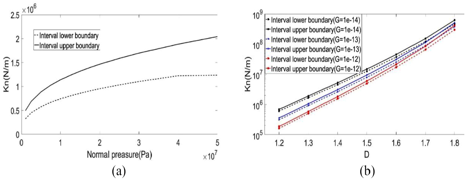
Relationship between normal pressure, fractal dimension, and interval of normal stiffness: (a) interval of normal stiffness versus P and (b) interval of normal stiffness versus D.

The variation ratio of every single D is determined to be 0.005 based on the above analysis. Then the relationship between the interval of K_n and fractal dimension D can be obtained. Figure 14(b) shows the interval of normal stiffness K_n increases with the increase of fractal dimension D, whereas it decreases with the increase of fractal roughness parameter G. The value of K_n calculated through the certain method proved to be included in the interval, meaning the roughness of the surface increases when D decreases, whereas the roughness increases when G increases, and the smaller the surface roughness, the bigger the stiffness. The conclusion is in agreement with the studies of Majumdar and Bhushan⁷ and Wang and Komvopoulos.⁸ Considering the variation ratio increases from 0.0647 to 0.1604, the uncertainty of D greatly influences K_n, especially for big values of D.

Figure 15(a) shows K_t tends to decrease when the interval parameters decrease from the maximum value to the minimum. $A_{l}$ greatly affects K_n whereas the effect of A_c is little due to that A_c is much smaller than $A_{l}$ . Figure 15(b) shows the simultaneous effect of D and A_l on K_t; it reaches the maximum value only when D and A_l take the maximum at the same time. The exact results are summarized in Table 6. The total tangential stiffness calculated by the certain method proved to be included in the interval, and the variation ratio is 0.2112.

Figure 15.

The effect of D, A_l, A_c on K_t: (a) separate effect of D, A_l, A_c on K_t and (b) simultaneous effect of D, A_l, A_c on K_t.

Table 6.

The interval of $K_{t}$ affected by uncertain parameters.

Influence factor	Interval	Central value	Rad	Variation ratio
D	[5.7053, 6.1077]	5.9065	0.2012	0.0341
A_l	[4.7761, 6.8504]	5.8133	1.0372	0.1784
A_c	[5.9048, 5.9048]	5.9048	0	0
D-A_l-A_c	[4.6147, 7.0857]	5.8502	1.2355	0.2112

Figure 16(a) shows the relationship between total tangential stiffness and normal pressure. Tangential stiffness tends to increase with the increase of normal pressure because the total real contact area A_l increases with the increase of normal pressure. Moreover, K_t increases slowly when the normal pressure is bigger than 4e7 Pa, and the stiffness interval widens with the increase of normal pressure for the variation ratio increases from 0.2071 to 0.2115. Figure 16(b) shows the interval of tangential stiffness K_t increases with the increase of fractal dimension D whereas it decreases with the increase of fractal roughness parameter G. The value of K_t calculated through the certain method can be proved to be included in the interval. Considering the variation ratio increases from 0.0630 to 0.1568, the uncertainty of D greatly affects K_t especially for big values of D. The reason agrees well with the analysis of K_n and the result is consistent with that in the studies of Majumdar and Bhushan⁷ and Wang and Komvopoulos.⁸

Figure 16.

Relationship between normal pressure, fractal dimension, and interval of $K_{t}$ : (a) interval of tangential stiffness versus P and (b) interval of tangential stiffness versus D.

Conclusion

In this article, the Chebyshev interval method is presented to estimate the contact stiffness of bolted joint with uncertain parameters. The fractal dimension D and fractal roughness parameter G are considered as the uncertain parameters. Interval models of the uncertain parameters are introduced to the fractal model and the equations are solved through the Chebyshev interval method. Normal and tangential stiffnesses are calculated based on the fractal model in microscale, and the upper and lower boundaries of the normal and tangential stiffness are determined using the Chebyshev interval method. The results show that the interval of the stiffness increases with the increase of fractal dimension D, whereas it decreases with the fractal roughness parameter G. The results are in good agreement with the referenced papers. Moreover, the variation ratio of the normal stiffness is 0.1604, the variation ratio of tangential stiffness is 0.1568, and thus, it is big enough to change the dynamic behavior of bolted joints. For the bolted joint systems, the variation ratio must be considered to enhance the reliability and reduce the system failure probability in design, manufacturing, and assembly processes.

Footnotes

Handling Editor: Zuzana Murčinková

Declaration of conflicting interests

The author(s) declared no potential conflicts of interest with respect to the research, authorship, and/or publication of this article.

Funding

The author(s) disclosed receipt of the following financial support for the research, authorship, and/or publication of this article: This research is supported by National Science and Technology Major Project of China (2018ZX04032002-002), Beijing major science and technology projects (Z181100003118001), Beijing Municipal Education Commission Science and Technology Project (KM201710005016).

ORCID iDs

Yongsheng Zhao

Zhifeng Liu

References

Ibrahim

Pettit

. Uncertainties and dynamics of bolted joints and other fasteners. J Sound Vib 2005; 279(35): 857–936.

Ren

Beards

. Identification of joint properties of a structure using FRF data. J Sound Vib 1995; 186(4): 567–587.

Jiang

Zheng

. A contact stiffness model of machined plane joint based on fractal theory. J Tribol 2010; 132: 011401.

Wang

Zheng

. Joint dynamic properties identification with partially measured frequency response function. Mech Syst Signal Pr 2012; 27: 499–512.

Majumdar

Tien

. Fractal characterization and simulation of rough surfaces. Wear 1990; 136(2): 313–327.

Ausloos

Berman

. A multivariate Weierstrass-Mandelbrot function. P Roy Soc Lond A Mat 1985; 400(1819): 331–350.

Majumdar

Bhushan

. Fractal model of elastic-plastic contact between rough surfaces. J Tribol 1991; 113(1): 1–11.

Wang

Komvopoulos

. A fractal theory of the interracial temperature distribution in the slow sliding regime: part II—multiple domains, elastoplastic contacts and applications. J Tribol: T ASME 1994; 116(4): 824–832.

Yan

Komvopoulos

. Contact analysis of elastic–plastic fractal surfaces. J Appl Phys 1998; 84(7): 3617–3624.

10.

Gonzalez-Valadez

Baltazar

Dwyer-Joyce

. Study of interfacial stiffness ratio of a rough surface in contact using a spring model. Wear 2010; 268(3/4): 373–379.

11.

Daisuke

Takahiro

Atsushi

, et al. Stiffness model of machine tool supports using contact stiffness. Precis Eng 2013; 37(3): 650–657.

12.

You

Chen

. A static friction model for the contact of fractal surfaces. Proc IMechE, Part J: J Engineering Tribology 2010; 224(5): 513–518.

13.

Zhao

Yang

Cai

, et al. Surface contact stress-based nonlinear virtual material method for dynamic analysis of bolted joint of machine tool. Precis Eng 2016; 43: 230–240.

14.

Grzejda

. Determination of bolt forces and normal contact pressure between elements in the system with many bolts for its assembly conditions. Adv Sci Technol Res J 2019; 13(1): 116–121.

15.

Wang

Qiu

. Modified perturbation method for eigenvalues of structure with interval parameters. Sci China Phys Mech Astron 2015; 58(1): 1–9.

16.

Wang

, et al. Reliability-based design optimization under mixture of random, interval and convex uncertainties. Arch Appl Mech 2016; 86(7): 1341–1367.

17.

Bickford

. An introduction to the design and behavior of bolted joints. 2nd ed. New York: Marcel Dekker, 1990.

18.

Xiu

Karniadakis

. The Wiener–Askey polynomial chaos for stochastic differential equations. SIAM J Sci Comput 2002; 24: 619–644.

19.

Yin

Lee

Chen

, et al. Efficient random field uncertainty propagation in design using multiscale analysis. J Mech Design 2009; 131(2): 021006.

20.

Kaufmann

Gupta

. Introduction to fuzzy arithmetic: theory and applications. J Franklin Inst 1986; 321(3): 189–190.

21.

Buckley

Feuring

. Fuzzy differential equations. Fuzzy Set Syst 2002; 110: 43–54.

22.

Mikaeilvand

Khakrangin

. Solving fuzzy partial differential equations by fuzzy two-dimensional differential transform method. Neural Comput Appl 2012; 21(1): 307–312.

23.

Lin

Stadtherr

. Deterministic global optimization for dynamic systems using interval analysis. In: Proceedings of the 12th GAMM—IMACS international symposium on scientific computing, computer arithmetic and validated numerics (SCAN 2006), Duisburg, 26–29 September 2006. New York: IEEE.

24.

Luo

Sun

, et al. An uncertain multidisciplinary design optimization method using interval convex models. Eng Optim 2012; 45: 1–23.

25.

Lü

. Stability analysis and improvement of automotive disc brake based on interval analysis. Automot Eng 2016; 38: 317–312.

26.

Moore

. Interval analysis. Englewood Cliffs, NJ: Prentice Hall, 1996.

27.

Nedialkov

Jackson

. A new perspective on the wrapping effect in interval methods for initial value problems for ordinary differential equations. In: Kulisch

Lohner

Facius

(eds) Perspectives on enclosure methods. New York: Springer, 2001, pp. 219–263.

28.

Berz

Makino

. Suppression of the wrapping effect by Taylor model-based verified integrators: long-term stabilization by shrink wrapping. Int J Diff Eq Appl 2006(4): 385–403.

29.

Han

Jiang

Gong

, et al. Transient waves in composite-laminated plates with uncertain load and material property. Int J Numer Method Eng 2008; 75(3): 253–274.

30.

Luo

Zhang

, et al. Interval uncertain method for multibody mechanical systems using Chebyshev inclusion functions. Int J Numer Method Eng 2013; 95(7): 608–630.

31.

Hanss

Oexl

Gaul

. Identification of a bolted-joint model with fuzzy parameters loaded normal to the contact interface. Mech Res Commun 2002; 29(2): 177–187.

32.

Guo

Zhang

. Identification of the mechanical joint parameters with model uncertainty. Chin J Aeronaut 2005; 18(1): 47–52.

33.

Norrick

. Statistical consideration of uncertainties in bolted joints of the drive train of sheet-fed offset printing presses. Appl Mech Mater 2015; 807: 3–12.

34.

Jiang

Shao-Qing

Shi

, et al. Contact interface parameter identification of bolted joint structure with uncertainty using thin layer element method. Eng Mech 2015; 32(4): 220–227.

35.

Seibel

Japing

Schlattmann

. Uncertainty analysis of the coefficients of friction during the tightening process of bolted joints. J Uncertain Anal Appl 2014; 2(1): 21.

36.

Imamovic

Hanafi

. Assessment of uncertainty quantification of bolted joint performance. In: Barthorpe

Platz

Lopez

(eds) Model validation and uncertainty quantification, vol. 3. New York: Springer, 2017.

Interval estimation for contact stiffness of bolted joint with uncertain parameters

Abstract

Keywords

Introduction

Mechanism of the three-dimensional fractal contact model

Total real contact area and load

Normal and tangential stiffness model of joint surface

Normal stiffness of joint surface

Tangential stiffness of joint surface

Uncertainty parameters of the bolted joints

The uncertain parameters D and G

Uncertainty of bolted joints using interval parameters

The basic definitions of interval arithmetic

Chebyshev inclusion function

The effect of interval parameters on the stiffness of bolted joints

Effects of D and G on Ac and Al

Effects of D and G on Ac

Effect of D and G on Al

The effect of uncertain parameters on the stiffness of bolted joints

Conclusion

Footnotes

Declaration of conflicting interests

Funding

ORCID iDs

References

Effects of D and G on A_c and A_l

Effects of D and G on A_c

Effect of D and G on A_l