Sage Journals: Discover world-class research

Abstract

The analysis of fluid flow near the wellbore region of a hydrocarbon reservoir is a complex phenomenon. The pressure drop and flow rates change in the near wellbore with time, and the understanding of this system is important. Besides existing theoretical and experimental approaches, computational fluid dynamics studies can help understanding the nature of fluid flow from a reservoir into the wellbore. In this research, a near wellbore model using three-dimensional Navier–Stokes equations is presented for analyzing the flow around the wellbore. Pressure and velocity are coupled into a single system which is solved by an algebraic multigrid method for the optimal computational cost. The computational fluid dynamics model is verified against the analytical solution of the Darcy model for reservoir flow, as well as against the analytical solution of pressure diffusivity equation. The streamlines indicate that the flow is radially symmetric with respect to the vertical plane as expected. The present computational fluid dynamics investigation observes that the motion of reservoir fluid becomes nonlinear at the region of near wellbore. Moreover, this nonlinear behavior has an influence on the hydrocarbon recovery. The flow performance through wellbore is analyzed using the inflow performance relations curve for the steady-state and time-dependent solution. Finally, the investigation suggests that the Navier–Stokes equations along with a near-optimal solver provide an efficient computational fluid dynamics framework for analyzing fluid flow in a wellbore and its surrounding region.

Keywords

Three-dimensional Navier–Stokes equations multigrid technique hydrocarbon reservoir nonlinear flow near wellbore reservoir inflow performance relation

Introduction

In the petroleum industry, the fluid flow phenomena at the vicinity of a wellbore are very important since most of the important quantities such as pressure drop, flow rate, formation damage, and so on are expected in this region.¹ In fact, the flow near a wellbore is more complex than the reservoir region far away from wellbore and could be nonlinear since sudden pressure drop can occur due to natural or artificial fractures or high permeable formation or perforation tunnels.^2,3 Darcy’s equation describes reservoir fluid flow in the regions where the flow phenomena are linear. In contrast, Forchheimer equation describes nonlinear fluid flow through porous media.^4–7 Nonlinear flow behavior in the near wellbore regions may have a significant influence on oil and gas production of the hydrocarbon reservoir.^7–9 Holditch and Morse¹⁰ investigated the near wellbore fluid flow using a model of fractured porous media, and concluded that over prediction of the flow rates happened when the linear equation was considered. Their study also showed that the hydrocarbon production had a 50% decline over the life of the well when the nonlinearity of the flow was neglected. Therefore, further research can be performed using three-dimensional (3D) Navier–Stokes equations (NSE) toward the study of near wellbore fluid flow.

Most of the existing models assume steady-state flow in the study of oil and gas flows of a reservoir.^11,12 In fact, during the production stage, the flow behavior becomes complex and pressure changes with time which has an influence on the productivity index.^11,13,14 Note that the productivity index is the relation among the flow rates of a well and pressures of wellbore and reservoir. Moreover, time-dependent nonlinear flow has significant influence on the inflow performance which affects the productivity index. Thus, the time-dependent models based on the NSE are more reliable since they cover the detailed physics of the flow, including linear and nonlinear flow properties.^11,15 A brief literature review shows that there is a growing interest to use the NSE in the field of petroleum industry. Narsilio et al.¹⁶ investigated various reservoir properties using the NSE. Ahammad et al.¹⁷ studied fluid flows through porous media using the NSE. Ahammad and Alam¹⁸ investigated miscible fluid flow through porous media using the NSE. Therefore, the NSE can be used to study reservoir flow in order to optimize the hydrocarbon production.¹⁶ Appropriate techniques and algorithms help to accurately solve this model to study flow in hydrocarbon reservoir.¹¹

Recently, computational fluid dynamics (CFD) has attracted researchers to study the fluid flow in a hydrocarbon reservoir. The availability of high performance multicore computing resources has made it possible to utilize the NSE for CFD investigations of some technological aspects of hydrocarbon reservoirs. Byrne et al.¹⁹ studied the fluid flow through a perforated open-hole tunnel of a vertical well using CFD methodology. The formation damage of asymmetric distribution around a well was simulated with CFD by Byrne et al.¹⁴ Molina and Tyagi³ performed a CFD investigation to study the fluid flow for the different formation layers and Frac-Paking zone. Szanyi et al.²⁰ studied a near wellbore of a horizontal well for steady-state flow using a pressure-based (segregated) on control volume technique with NSE.

The present investigation explores the benefits of using 3D NSE to study pressure drop and fluid flow phenomena at the near well-bore. The aim of this research is further advancement of the application of the 3D NSE with CFD methodology in the field of petroleum industry. In this regard, the results based on NSE will be compared with Darcy and Forchheimer equations.

In section “CFD model for near wellbore simulation,” we present the important techniques for investigating fluid flow in the vicinity of a vertical wellbore. Notably, the CFD analysis of near wellbore region requires appropriate mathematical formulations. We briefly outline the mathematical equations for the flow through porous media which represent the near wellbore flow with necessary boundary conditions in sections “Governing equation for flow through porous media” and “Boundary conditions.” Sections “Pressure calculation using Darcy model” and “Pressure calculation using pressure diffusivity equation” describe the analytical solution to calculate pressure for steady-state and time-dependent conditions, respectively. In section “Solution technique of NSE for flow in porous media for linear and nonlinear flow,” the potential solution technique to solve the model equation for the flow through porous media based on NSE in the is described. The numerical simulations are analyzed in section “Numerical results and discussions.” The model is verified with existing analytical solutions. Finally, the performance of the model is investigated and analyzed with pressure drop and inflow performance relationship (IPR) curves studies, and flow direction is studied with streamline behavior and discussed in the numerical results section.

Methodology

CFD model for near wellbore simulation

The diagram of a commonly used computational design for a near wellbore simulation is shown in Figure 1. The average length, height, and wells depth of a hydrocarbon reservoir are $3000, 100$ , and $477 m$ , respectively.¹² To design a near wellbore model, one needs to consider the reasonable scale of the reservoir, for example, Chupin et al.¹² assumed length $350 m$ , thickness $26.7 m$ , and wells depth $477 m$ to model a near wellbore reservoir simulation. Chupin et al.¹² also considered 153 lateral gird blocks for the reservoir of size $3000 m \times 3000 m \times 30 m$ , and 100 grid blocks for a near wellbore reservoir of size $350 m \times 350 m \times 26.7 m$ . Thus, a single grid block has the average lateral size of $20 m$ for the full scale reservoir and $3.5 m$ for near wellbore reservoir model. In fact, to capture the real flow, this size is not sufficient enough as the typical length and diameter of a perforation tunnel is less than $3.5 m$ . Therefore, we need to choose a near wellbore dimension and grid size so that the near wellbore flow can be captured. Furthermore, Chupin et al.¹² mentioned that the sufficient distance of a wellbore from a reservoir is $10 to 100 m$ to simulate a near wellbore reservoir model. We consider a near wellbore reservoir with a reasonable scale in this research so that computational cost can be optimized with sufficient smaller grid size. Here, we also assume a hydrocarbon reservoir which is enclosed by the impermeable geological formation at the top and bottom. In Figure 1(b), $r_{w}$ and $r_{e}$ represent wellbore and near wellbore reservoir radius, respectively. The present computational domain can be extended as desired size and shape as convenient; moreover, the formation damage zone around wellbore can be included as well.

Figure 1.

(a) A computational design of reservoir along with a vertical wellbore and (b) the near wellbore region of a reservoir which is similar to the rest of the simulation in this research.

Governing equation for flow through porous media

We consider the volume averaged NSE for slightly compressible flow to investigate the flow behavior in the near wellbore region of a reservoir as (see Szanyi et al.,²⁰ ANSYS,²¹ Azadi et al.,²² Ahammad and Alam¹⁸)

\frac{\partial ρ}{\partial t} + \frac{\partial (ρ u_{j})}{\partial x_{j}} = 0

(1)

\begin{matrix} ρ (\frac{\partial u_{i}}{\partial t} + u_{j} \frac{\partial u_{i}}{\partial x_{j}}) = - \frac{\partial P}{\partial x_{i}} + \frac{\partial τ_{ij}}{\partial x_{i}} + ρ g_{i} + F_{i}, \\ (i, j = 1, 2, 3) \end{matrix}

(2)

where $τ_{ij} = μ ((\partial u_{i} / \partial x_{j}) + (\partial u_{j} / \partial x_{i}))$ and $F_{i}$ are the momentum sink which is a combination of a viscous loss and an inertia loss due to porous media. Note that the inertial force (i.e. nonlinear flow) may have a significant effect on the near wellbore fluid flows. The total momentum sink is defined as

F_{i} = - \frac{μ}{K} u_{i} - β \frac{ρ}{2} | u | u_{i}

(3)

in the expression for $F_{i}$ , $β$ is known an inertia resistance factor that has a unit of inverse of the length. In the study by Khaniaminjan and Goudarzi,²³ several formulations of $β$ were studied. All of the models mentioned in the study by Khaniaminjan and Goudarzi²³ are considered the unit of $β$ as $m^{- 1}$ or $f t^{- 1}$ whereas the unit of $K$ is $mD$ . In the present investigation, we choose the following $β$ factor

β = \frac{17.2 \times 10^{10}}{K^{1.76}}

(4)

Here, the unit of $K$ is $mD$ and the exponent of 1.76 is applied to the magnitude of the unit of $K$ so that $β$ has an unit of $m^{- 1}$ (see details in Khaniaminjan and Goudarzi²³).

Boundary conditions

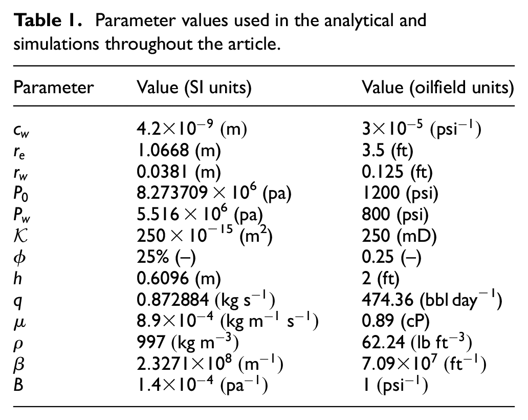
As shown in Figure 1(a), we consider a near wellbore region for the present CFD simulations. The dimension of the near wellbore reservoir and other parameters are listed in Table 1. We assume inlet at the outer boundary of the near wellbore region and outlet at the wellbore surface as described in section “CFD model for near wellbore simulation.” The boundary condition at the inlet of the present CFD simulations is

P (r_{e}, t) = P_{0}, t \geq 0

(5)

The boundary condition at the outlet is

r \frac{\partial P}{\partial r} = \frac{q μ}{2 π K h}, t > 0 and r = r_{w}

(6)

where a constant flow rate is presented.

Table 1.

Parameter values used in the analytical and simulations throughout the article.

Parameter	Value (SI units)	Value (oilfield units)
$c_{w}$	$4.2 \times 10^{- 9} (m)$	$3 \times 10^{- 5} (ps i^{- 1})$
$r_{e}$	1.0668 (m)	3.5 (ft)
$r_{w}$	0.0381 (m)	0.125 (ft)
$P_{0}$	8.273709 × 10⁶ (pa)	1200 (psi)
$P_{w}$	5.516 × 10⁶ (pa)	800 (psi)
$K$	250 × 10⁻¹⁵ (m²)	250 (mD)
$ϕ$	25% (–)	0.25 (–)
$h$	0.6096 (m)	2 (ft)
$q$	$0.872884 (kg s^{- 1})$	474.36 (bbl day⁻¹)
$μ$	$8.9 \times 10^{- 4} (kg m^{- 1} s^{- 1})$	0.89 (cP)
$ρ$	$997 (kg m^{- 3})$	$62.24 (lb f t^{- 3})$
$β$	$2.3271 \times 10^{8} (m^{- 1})$	$7.09 \times 10^{7} (f t^{- 1})$
$B$	$1.4 \times 10^{- 4} (p a^{- 1})$	$1 (ps i^{- 1})$

Initial pressure in the reservoir is assumed to be uniform, thus

P (r, 0) = P_{0}, r_{w} \leq r \leq r_{e}

(7)

Top and bottom layers of the computational domain are considered as wall, so no flow boundary condition is used here.

Pressure calculation using Darcy model

Assuming the flow is steady-state, and linear from reservoir end to wellbore surface, then classical Darcy model has the form

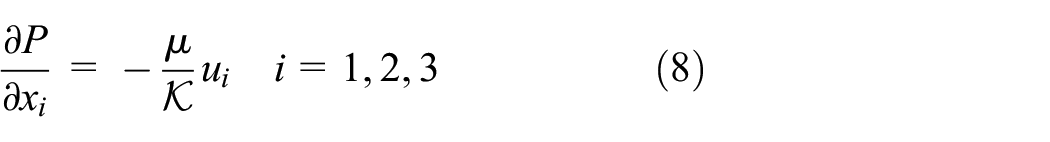
\frac{\partial P}{\partial x_{i}} = - \frac{μ}{K} u_{i} i = 1, 2, 3

(8)

For the isotropic reservoir, equation (8) can be written polar coordinate as

\frac{\partial P}{\partial r} = - \frac{q μ}{2 π r K h}, r ϵ [r_{w}, r_{e}]

(9)

Integration of equation (9) leads to the analytical solution of Darcy equation for a steady-state condition as²⁴

P = P_{w} + \frac{q μ}{h K} \ln (\frac{r}{r_{w}})

(10)

where $r, r_{w}, P_{w}, P$ , and $h$ are the reservoir radius, wellbore radius of the reservoir, wellbore pressure, reservoir pressure, and height of the reservoir, respectively. Converting to oilfield units, where $P$ and $P_{w}$ are in psi, $q$ is in STB/d, $μ$ is in cP, $K$ is in mD, $h$ is in ft, and $B$ is the formation volume factor to convert STB into bbl, in that case equation (10) becomes²⁴

P = P_{w} + 141.22 \frac{Bq μ}{h K} \ln (\frac{r}{r_{w}})

(11)

Pressure calculation using pressure diffusivity PD equation

As we assume that flow occurs in radial direction, the mass conservation equation for radial flow with true velocity is

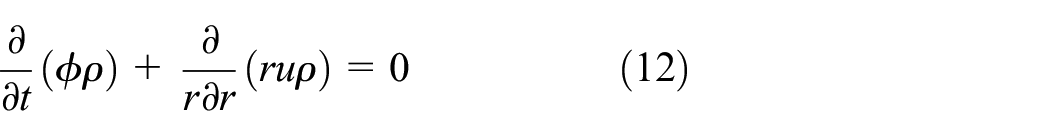
\frac{\partial}{\partial t} (ϕ ρ) + \frac{\partial}{r \partial r} (ru ρ) = 0

(12)

Darcy equation can be combined with mass conservation equation to obtain PD equation. Thus, combining Darcy equation, for example, equation (8) with the mass conservation equation (12), one-dimensional diffusivity equation for slightly compressible fluid takes the form as^8,25

\frac{\partial^{2} P}{\partial r^{2}} + \frac{1}{r} \frac{\partial P}{\partial r} + c_{r} {(\frac{\partial P}{\partial r})}^{2} = \frac{ϕ μ c_{t}}{K} \frac{\partial P}{\partial t}

(13)

where total compressibility $c_{t}$ is the sum of rock and fluid compressibility $c_{r} = (1 / ϕ) (\partial ϕ / \partial P)$ and $c_{f} = (1 / ρ) (\partial ρ / \partial P)$ , respectively. The solution of this equation describes pressure at any location, $r$ , at any time, $t$ , within the domain. This is a nonlinear partial differential equation and difficult to solve for an analytical solution. For simplification, one can neglect the nonlinear term in equation (13) by considering pressure variation is small,²⁶ then the equation (13) becomes

\frac{\partial^{2} P}{\partial r^{2}} + \frac{1}{r} \frac{\partial P}{\partial r} = \frac{1}{χ} \frac{\partial P}{\partial t}

(14)

which is known as the PD equation in reservoir studies, where $χ = K / ϕ μ c_{t}$ . Under the following assumptions, pressure can be calculated analytically from PD. The reservoir is isotropic and homogeneous in all directions, well produces at constant flow rate, the radius of the well is negligible compared to reservoir, the reservoir has uniform initial pressure, and the well drains an infinite area (i.e. $P \to P_{0}$ as $r \to \infty$ ). Under these conditions, pressure can be calculated from the equation (14) as

P (r, t) = P_{0} - \frac{q (t) μ}{4 π K h} \ln (\frac{2.25 t χ}{r^{2}})

(15)

Now converting the variables in oilfield units, the above equation becomes (see for details, chapter 2, p. 25, of Economides²⁴)

P (r, t) = P_{0} - \frac{162.6 Bq (t) μ}{K h} (lo g_{10} (\frac{t χ}{r^{2}}) - 3.23)

(16)

Solution technique of NSE for flow in porous media for linear and nonlinear flow

In the element-based finite volume method, the first discretization involves the spatial domain using a mesh. The generated mesh is used to construct finite volumes. The relevant quantities such as mass, momentum, and energy are expected to conserve on the mesh. Mesh generation is important in CFD simulations since capturing the physics of flow, accuracy, and convergence depends on mesh size and time step.²⁷ The meshing tools in ANSYS CFX v17.2 are used to generate the mesh in this research.

The discretization of the governing equation on a complex geometry is tricky. The higher resolution scheme based on the upwind method is used for the spatial discretization.²⁷ For the time integration, implicit backward Euler scheme is used since it is unconditionally stable.²⁷

ANSYS CFX uses the collocated grid where the values of all variables are calculated at the cell centers. This grid has the advantage of converting the mesh to other coordinate systems easily considering the complexity of the domain.²¹ Moreover, collocated grid arrangement stores the vector and scalar variables at the same locations, so it requires less computer memory.²⁸ However, this technique arises the pressure–velocity decoupling issue, and Rhie and Chow²⁹ interpolation method is used to handle the issue.^28,30 The velocity–pressure coupling solver is used in this research where the system of linear equations is solved using an algebraic multigrid technique. Algebraic multigrid technique transforms a system of discrete equations for a coarse mesh by summing the finer mesh equations. The process is performed on virtual grid cells during the iterations and re-refined the mesh to obtain an accurate solution. This technique is less expensive with higher convergence rates since the discretization of the nonlinear equations is solved only once on finer mesh.²⁷ The algorithm is implemented in ANSYS CFX and the advantage of this algorithm is utilized in this research. Here the algorithm is summarized as follows:

Step 1. Initialize with $Δ t$ and other parameter values.

Step 2. Take latest value of $u, v, w$ , and $P$ .

Step 3. Apply Rhie and Chow interpolation technique for $u, v, w$ , and $P$ .

Step 4. Solve the coupled system of equation for $u, v, w$ , and $P$ .

Step 5. Apply Algebraic Multigrid technique to solve the system of equations until convergence criteria fulfill.

Step 6. Solve the other variables of interest (if any).

Step 7. If time reaches at a maximum level then stop otherwise go back to step 2, and repeat the same.

IPR formulation

The present near wellbore model based on NSE is expected to perform as like other models such as PD equation. We study the IPR with the present numerical solutions using NSE. The IPR is defined as the relationship between the well production rate and flowing pressure of the well. It has importance to the production engineers since depending on this relation they have to adjust the pressure at separator or pipeline junction.²⁴ The IPR curves can be three types: steady state, transient, and pseudo-steady state. The IPR curves calculated by the present simulations will be compared to the analytical solution. First, we derive IPR formulation with the parameters listed in Table 1 for linear $(β = 0)$ flow simulations model. After utilizing the parameter values in equation (11), the IPR curve for steady state with no skin effect stands as

P_{w} = 1200 - 0.84 q_{ss}

(17)

where $q_{ss}$ is for flow rate in the case of steady-state condition. Now, deploying the parameter values from Table 1 to equation (16) for nonlinear flow (here, $c_{t} = c_{w}$ since we are using water and flow is single phase, and $β = 2.3271 \times 10^{8} m^{- 1}$ ) phenomena, the IPR curve of time-dependent model equation for nonlinear flow with no skin effect becomes

P_{w} = 1200 - \frac{q}{3.46} (lo g_{10} t + 6.15)

(18)

Numerical results and discussions

Near wellbore reservoir model setup

The present near wellbore model setup is verified with the Darcy equation and PD equation in the following sections.

Verification with Darcy model for steady-state condition

In this section, we consider NSE for linear flow model with the steady-state condition to simulate near wellbore flow for a simple case. As described in section “Methodology,” a simple homogeneous reservoir with a wellbore at the center is considered. The performance of CFD results with NSE is verified with the analytical solution of the Darcy equation (i.e. equation (11)).

Parameters for this simulation are chosen for an idealized hydrocarbon reservoir and the values are listed in Table 1 where water at 25°C is considered. In addition, we choose $β = 0$ so that inertia force is turn off in NSE (equation (2)) to make consistent with the Darcy model. Pressure profile is calculated from the present model and compared with the analytical solutions of the Darcy model (see Figure 2). Both solutions have a very good agreement, and the relative error is very small to distinguish both solutions. Thus, some data points of both solutions are measured with error analysis. The analysis indicates that the present model has a very close consistent result to the analytical solution with a maximum error of $0.45 %$ . This result indicates that the present model setup can be used to describe the underlying physics of fluid flow in a near wellbore reservoir.

Figure 2.

Validation of CFD model based on Navier–Stokes equations for linear model $(β = 0)$ with the analytical solution of Darcy equation for steady-state flow.

Verification with the solution of pressure diffusivity equation

According to a brief literature review, we see the near wellbore flow has a nonlinear tendency.^4–7 Here, we compare the pressure which is calculated using NSE for current numerical simulations with the analytical solution of PD. The parameter values for the simulations are listed in Table 1. The pressure is calculated using NSE for nonlinear $(β = 2.3271 \times 10^{8} m^{- 1})$ and linear $(β = 0)$ models, and is compared with the analytical solution of PD equation. The pressure profiles are drawn along the radial distance of the reservoir and presented in Figure 3. The results indicate that the pressure drop with respect to radial distance has a good match except at the wellbore region. We notice that the difference of pressure drop at the wellbore between linear model, that is, without inertia force and nonlinear, that is, with inertia force is about $344, 738 Pa \approx 50 psi$ . In addition, the difference of pressure drop between the analytical solution of PD equation and NSE equations with the nonlinear term is about $172, 369 Pa \approx 25 psi$ . The deflection of pressure drop compared to the linear and nonlinear model using the NSE, and the analytical solution of the PD equation may be the cause inertia force, that is, nonlinear term. We see in the Darcy equation—flow rate is linearly dependent with pressure drop and the analytical solution of PD is obtained by dropping the nonlinear term. This is the reason of deflection of pressure near the wellbore. This investigation indicates that the NSE with efficient CFD technique in the study of reservoir flow is promising.

Figure 3.

Comparison of pressure distributions calculated by NSE equations, and analytical solution of PD equation for nonlinear $(β = 2.3271 \times 10^{8} m^{- 1})$ and linear $(β = 0)$ , that is, Darcy model.

Flow characteristic at the near wellbore

In this section, we discuss the fluid flow phenomena at the near wellbore region for different flow rate scenarios.

Flow behavior at near wellbore region

The fluid flows start from far away from the wellbore region of a reservoir where the flow obeys Darcy’s law, and the fluid pressure decreases as the fluid moves toward the wellhead through the wellbore. Mostly, the pressure drop occurs at the near wellbore, and the mean flow of a reservoir fluid is along the radial direction which causes fluid velocity to increase continuously at wellbore region.² The flow phenomena at the near wellbore of an idealized reservoir are investigated with different flow rate scenarios considering linear and nonlinear flow models. The parameter values are listed in Table 1 with variation of flow rate, $q$ and controlling $β = 2.3271 \times 10^{8} m^{- 1}$ for nonlinear flow. Pressure drop is calculated at the wellbore surface for different flow rates in both cases. The pressure difference data are plotted with respect to flow rates and presented in Figure 4 for both linear and nonlinear flow models with least square curve fitting process. The polyfit tool is used for the curve fitting process in MATLAB code while plotting the simulations data in post-process to check nature of the relation of pressure drop with flow rate. A quadratic curve is well fitted with the data for nonlinear flow whereas a curve with degree one is fitted with the linear flow. Equation (2) with $β = 2.3271 \times 10^{8} m^{- 1}$ is nonlinear and the curve fitting equation, $dp = 33.072 q^{2} + 472.4313 q + 0.1599$ with $R^{2} = 1$ , is also nonlinear. On the other hand, equation (2) with $β = 0$ is considered as Darcy flow which is linear and curve fitting equation, $dp = 473.1582 q - 0.06598$ with $R^{2} = 1$ , is also linear. Note that when the flow rate is small, linear and nonlinear models have the same behavior, and the difference is noticeable for a higher flow rate. The CFD results with the value of the prescribed parameter indicate that the relationship between pressure drop and flow rate remains linear until the mass flow rate reaches 0.6 kg s⁻¹. After that, the relation between flow rate and pressure drop is visible, that is, linear and nonlinear. This analysis indicates NSE can explain fluid flow phenomena at the near wellbore region. This investigation helps production engineer and well management with more ideas of flow behavior near wellbore region in that case of linear or nonlinear.

Figure 4.

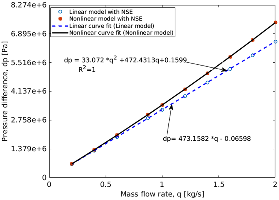
Comparison of pressure drop as a function of flow rate at the wellbore surface.

The pressure drop at the wellbore depends greatly on the well flow rate, and the life of the reservoir depends on the optimum production rate. Over time, the flow and pressure decreasing rates depend upon the various reservoir parameters. This study focuses on the near wellbore flow phenomena where the flows are mostly nonlinear. We see the pressure drop increases with time for both linear and nonlinear flows, shown in Figure 5. The prediction of pressure drop by linear flow model at the early time is about $6.378 \times 10^{6} Pa \approx 925 psi$ , whereas $7.2395 \times 10^{6} Pa \approx 1050 psi$ for the nonlinear model. The trend continues until the final time of the simulations and at the end, the difference of pressure drop between the two models is $8.619 \times 10^{5} Pa \approx 125 psi$ . This indicates that the flow rates at the near wellbore will be decreased gradually over the production period, and it will be more for the nonlinear model compared to linear model—this information supports the findings of Wang and Sheng.³¹

Figure 5.

Pressure drop analysis at the near wellbore with linear $β = 0$ and nonlinear models $(β = 2.3271 \times 10^{8} m^{- 1})$ .

Flow direction

Here, we consider nonlinear model with $β = 2.3271 \times 10^{8} m^{- 1}$ to investigate the flow pressure pattern and flow direction.

Streamlines may give a more detailed description of mass flow across the wellbore region since they provide information both on the magnitude and direction of flow velocity at a given point in time. The streamlines are plotted along a vertical plane of the reservoir and presented in Figure 6. We see the magnitude of the velocity is higher at the near wellbore compare to the reservoir end. The fluid velocity is gradually increasing from the reservoir end to the wellbore region. This indicates the fluid is flowing in a constant flow rate to the radial direction of the reservoir.

Figure 6.

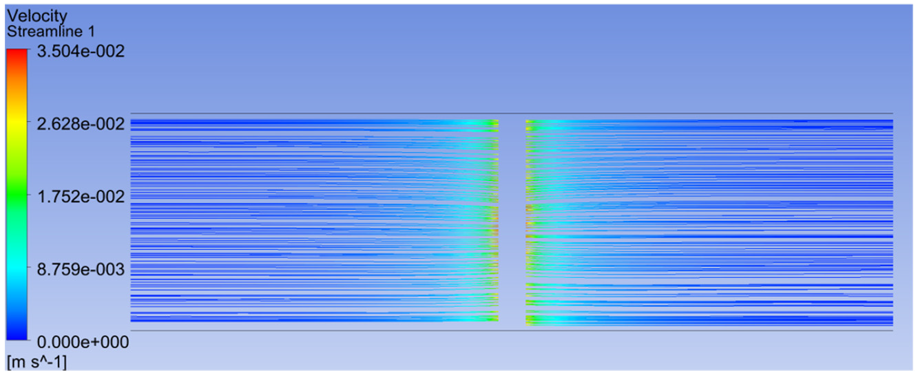
The streamlines along a vertical cross section of the domain representing flow direction.

Inflow performance relation analysis

In this section, we consider linear and nonlinear model based on NSE to investigate the inflow performance at the near wellbore. The inflow performance relation is investigated for two scenarios: linear and nonlinear flow models. First case, we consider CFD simulations for linear model $β = 0$ using NSE, and the results are compared with the analytical solutions (i.e. equation (17)). We find that the IPR curve generated from CFD solution has a good agreement until flow rate $q = 0.92007 kg s^{- 1} \approx 500 bbl da y^{- 1}$ . Further, the deflection is noticed for the higher flow rate, that is, $q = 1.10408 kg s^{- 1} \approx 600 bbl da y^{- 1}$ , in this case, the decline pressure is about $137, 895 Pa \approx 20 psi$ which is $3 %$ (see Figure 7(a)). In the second case, we investigate the application of the proposed CFD model based on NSE for the nonlinear model for inflow performance analysis. Three-time durations, $t = 0.003, 0.008$ , and $0.014 h$ , are taken into account for the present study. Following equation (18), the time-dependent IPRs are calculated and then compared against the present CFD data (see Figure 7(b)). The transient IPR curves for present CFD simulations have a very good agreement with the theoretical results. There is only a slight deflection for higher flow rate $(q = 1.10408 kg s^{- 1} \approx 600 bbl da y^{- 1})$ at the final time $0.014 h$ which is about $3.7 %$ difference of pressure, and this is reasonable. Thus, the simulation time $0.008 h$ can be the optimal time duration for a flow to be steady-state in the present idealized reservoir condition.

Figure 7.

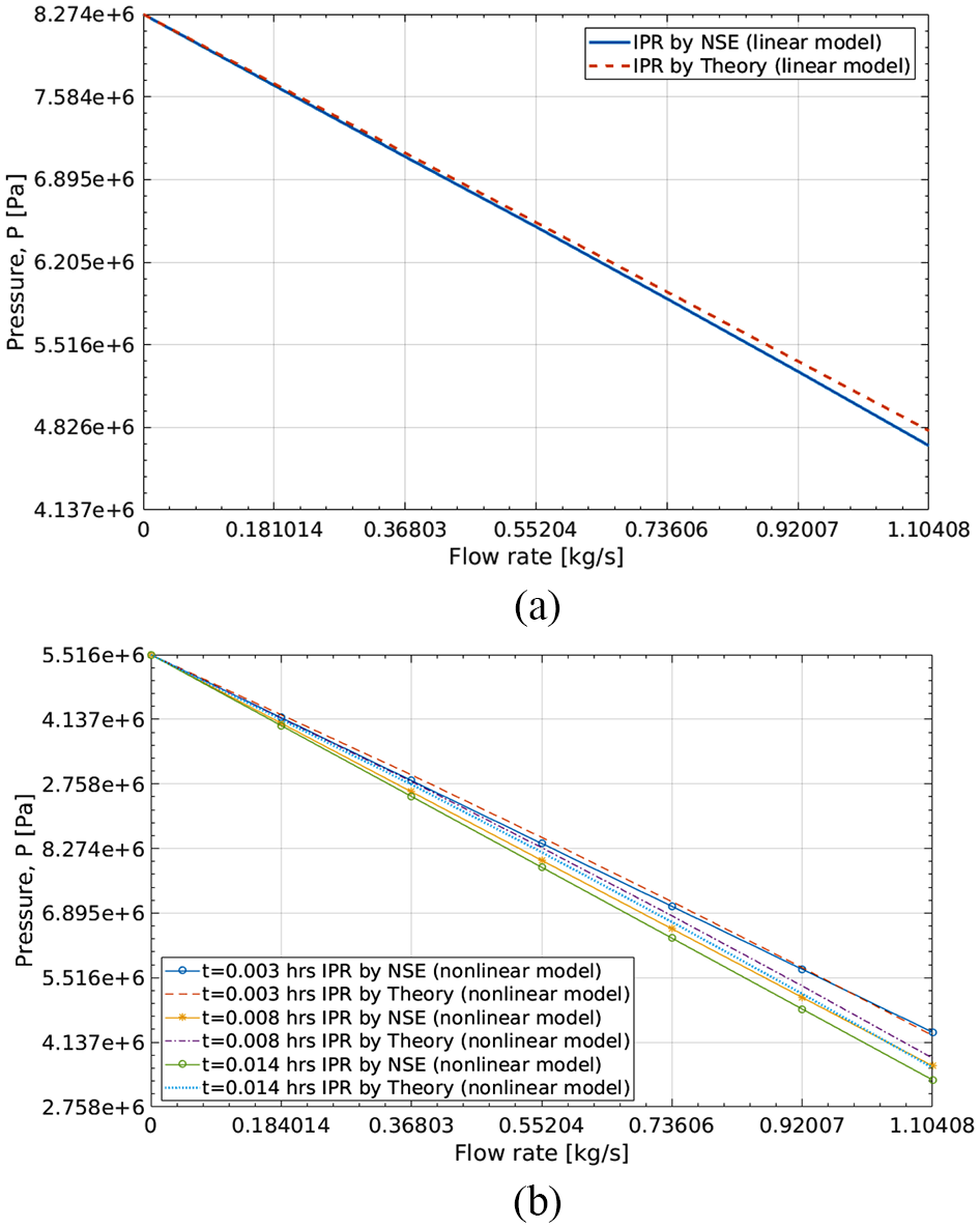
Comparison of the IPR curves: (a) steady-state IPR curves with theory and (b) time-dependent IPR curves with theory.

The proposed CFD modeling based on NSE can be used for better determination of the future behavior of a reservoir and can explain the various production scenarios of a reservoir and help production engineering to maintain the pressure at separator or transport pipeline.

Pressure distribution analysis using NSE

The CFD modeling based on NSE delivers the promising results, including pressure and velocity distribution in the near wellbore model as well as 3D flow patterns. In this section, we discuss the characteristics of pressure distribution for different conditions such as flow rates. The pressure distribution help understand the process of reservoir fluid flow through a reservoir to the wellbore.

Different flow rates for linear flow model

The pressure distribution for linear flow model ( $β = 0$ in model equation) is studied for three different flow rates such as $q = 0.36803$ , $0.73606$ , and $1.10408 kg s^{- 1}$ in the case of steady-state condition. The pressure contours for each case are plotted along a vertical plane, that is, $y = 0$ and the results are exhibited in Figure 8. The pressure at the reservoir ends is gradually decreasing toward around the wellbore. This means that the reservoir fluid is gradually moving to the wellbore. To quantify the pressure drop at the wellbore, we draw pressure profiles for three cases along a horizontally mid-line of the reservoir (Figure 9). We see that there is a pressure drop about $7.075 \times 10^{6} Pa$ for the flow rate of $0.36803 kg s^{- 1}$ , $5.878 \times 10^{6} Pa$ for flow rate $0.73606 kg s^{- 1}$ , and $4.636 \times 10^{6} Pa$ for flow rate $1.10408 kg s^{- 1}$ . The results show that pressure drop increases for higher production rate, this means for higher production of a well will reduce the reservoir life. Furthermore, the pressure distribution in the near wellbore shows that the pressure gradient is adverse in the near wellbore which indicates the sudden changes in the velocity field. The results indicate that velocity increases at the near wellbore for the high flow rate compared to low flow rate. This argument supports the sudden pressure drop at the wellbore region.

Figure 8.

Contour plots of pressure distribution along a vertical plane of the reservoir for steady-state linear model $(β = 0)$ condition at different flow rates.

Figure 9.

Pressure profiles for different flow rates of steady-state linear model $(β = 0)$ simulations.

Different flow rates for nonlinear flow model

In this section, we study the influences of production rates and production time on the fluid flows of a reservoir, and pressure drop at the near wellbore using the nonlinear model $(β = 2.3271 \times 10^{8} m^{- 1})$ with NSE. Here, we also consider three different flow rates: $(0.36803, 0.73606, and 1.10408 kg s^{- 1})$ . We plot pressure contour of each case of flow rate for three time intervals: $0.003$ , $0.008$ , and $0.014 h$ . The influences of production rates are the same as the linear model but more pressure drop occur for the nonlinear model. The pressure drop at the near wellbore is decreasing with respect to time increase for all three cases (Figure 10). This means that the reservoir fluid is gradually moving to the wellbore with time. In Figure 10, the pressure changes are only visible in the legend of the contour plots. We draw pressure profiles for all cases of simulations presented in Figure 10 along the mid-line of the reservoir. The results are displayed in Figure 11 with zoom in for more visibility of the differences. We notice two features in all cases: pressure drops gradually near the wellbore, and it converges with the increase of time. Furthermore, when the flow rate increases, the pressure drop near the wellbore is higher than the less flow rate, shown in Figure 11(d). This pressure drop at the near wellbore indicates that the velocity at the near wellbore increases for the higher flow rate compared to low flow rate. This supports the accurate pressure calculation in the study of reservoir fluid flows using NSE equations.

Figure 10.

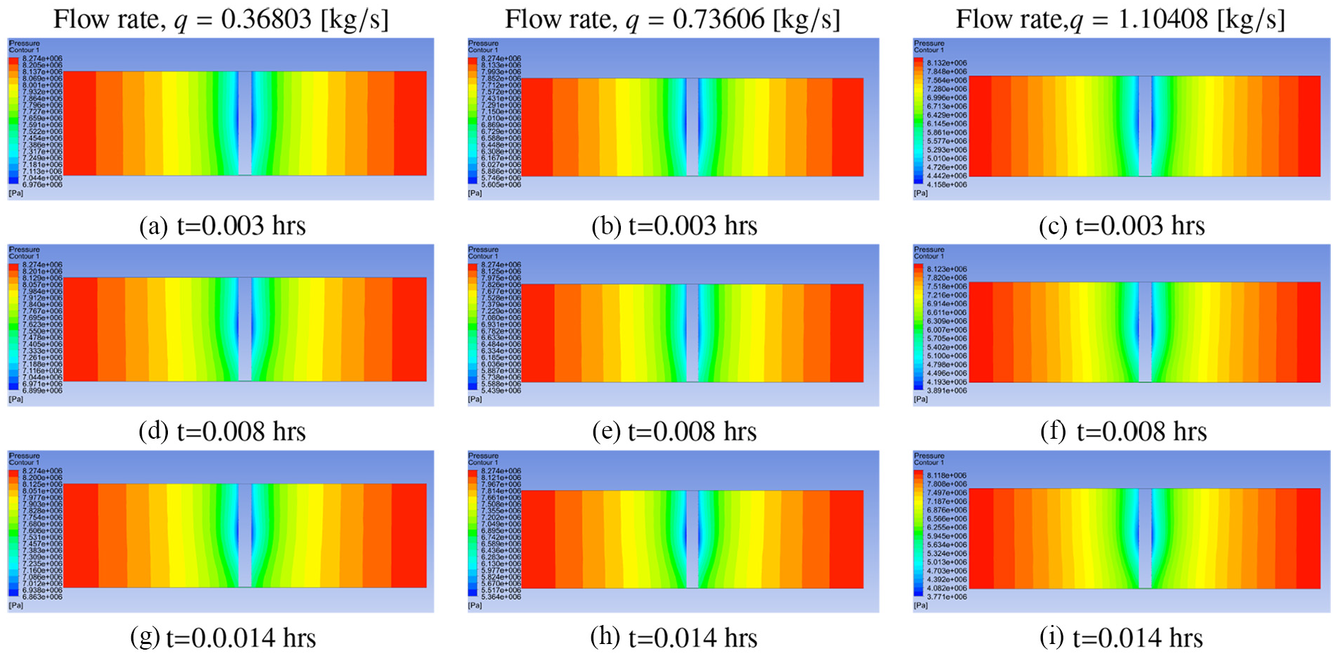
Pressure distribution contour plot along a vertical plane for different flow rates for the simulations of nonlinear model $(β = 2.3271 \times 10^{8} m^{- 1})$ : (a–c) t = 0.003 h, (d–f) t = 0.008 h, and (g–i) t = 0.014 h.

Figure 11.

Pressure distributions as a function of radial distance to the wellbore for nonlinear flow model $(β = 2.3271 \times 10^{8} m^{- 1})$ : (a) for the flow rate, $q = 0.36803 kg s^{- 1}$ , (b) for the flow rate, $q = 0.73606 kg s^{- 1}$ , (c) for the flow rate, $q = 1.10408 kg s^{- 1}$ , and (d) for the fixed time $t = 0.014 h$ with different flow rates.

Finally, we follow that higher pressure drop occurs for the higher flow rate. This indicates to the production engineers that more attention needs to be drawn to maintain optimal pressure at all stages. This is the sign of turbulent flow at the wellbore for high flow rate, and nonlinear model is more suitable to study flow at near wellbore.

Conclusion and future work

This study investigates modeling of fluid flow phenomena around the near wellbore of a reservoir using 3D NSE. The pressure-based velocity–pressure coupled solver is applied to get a robust, accurate numerical solution of NSE. We verify the present model with existing analytical solutions and other models. Then, we study the nature of the fluid flows around the near wellbore for a steady-state and time-dependent solution. In this study, we extensively investigate the flow behavior near the wellbore with pressure, streamlines, and IPR curve analysis. This study will help to understand the pressure drop near the wellbore for different flow scenarios and the IPR utility in solving everyday production problems and confirm the possibility of time-dependent IPR curves. Time-dependent IPR curves are dependent on the production history, so it helps for future forecasting of the reservoir life. The extension of this model is under process to study the formation damage with different skin zones using coupled wellbore-skin-reservoir approach and transient flow analysis at the near wellbore of a reservoir. In addition, the model can be extended for a horizontal well with formation damage and other features such as sand control.

Footnotes

Appendix 1

Handling Editor: James Baldwin

Declaration of conflicting interests

The author(s) declared no potential conflicts of interest with respect to the research, authorship, and/or publication of this article.

Funding

The author(s) disclosed receipt of the following financial support for the research, authorship, and/or publication of this article: We acknowledge the financial support from the National Science and Research Council (NSERC), Canada and Memorial University of Newfoundland, Canada. M.A.R. also acknowledges Qatar National Research Fund (a member of the Qatar Foundation) for the grant NPRP10-0101-170091. Statements made herein are solely the responsibility of the author. M.J.A. acknowledges School of Graduate Studies, Memorial University of Newfoundland, Canada for scholarships.

ORCID iDs

Mohammad Jalal Ahammad

Mohammad Azizur Rahman

References

Dake

. The practice of reservoir engineering. Revised ed., Vol. 36. Amsterdam: Elsevier, 2001.

Jin

Chen

. Highly compressible porous media flow near a wellbore: effect of gas acceleration. J Fluid Eng 2012; 134: 011301.

Molina

Tyagi

. A computational fluid dynamics approach to predict pressure drop and flow behavior in the near wellbore region of a frac-packed gas well. In: Proceedings of the ASME 2015 34th international conference on ocean, offshore and arctic engineering, St. John’s, NL, Canada, 31 May–5 June 2015, pp.V010T11A023–V010T11A023. New York: American Society of Mechanical Engineers.

Firoozabadi

Katz

. An analysis of high-velocity gas flow through porous media. J Petrol Technol 1979; 31: 211–216.

Svec

Engler

, et al. Modeling and simulation of the wafer non-Darcy flow experiments. In: Proceeding of the SPE western regional meeting, Bakersfield, CA, 26–30 March 2001, pp.1–11. Richardson, TX: Society of Petroleum Engineers.

Y-S

Lai

Miskimins

, et al. Analysis of multiphase non-Darcy flow in porous media. Transport Porous Med 2011; 88: 205–223.

Song

Cao

, et al. Numerical research on CO₂ storage efficiency in saline aquifer with low-velocity non-Darcy flow. J Nat Gas Sci Eng 2015; 23: 338–345.

Rahman

Mustafiz

Biazar

, et al. Investigation of a novel perforation technique in petroleum wells—perforation by drilling. J Frankl Inst 2007; 344: 777–789.

Ahammad

Rahman

Zheng

, et al. Numerical investigation of two-phase fluid flow in a perforation tunnel. J Nat Gas Sci Eng 2018; 55: 606–611.

10.

Holditch

Morse

. The effects of non-Darcy flow on the behavior of hydraulically fractured gas wells (includes associated paper 6417). J Petrol Technol 1976; 28: 1–169.

11.

Shi

Holmes

Durlofsky

, et al. Drift-flux modeling of two-phase flow in wellbores. SPE J 2005; 10: 24–33.

12.

Chupin

Haugset

, et al. Integrated wellbore/reservoir model predicts flow transients in liquid-loaded gas wells. In: Proceeding of the SPE annual technical conference and exhibition, Anaheim, CA, 11–14 November 2007, pp.1–11. Richardson, TX: Society of Petroleum Engineers.

13.

Ding

. Transient pressure solution in the presence of pressure drop in the wellbore. In: Proceeding of the SPE annual technical conference and exhibition, Houston, TX, 3–6 October 1999, pp.1–12. Richardson, TX: Society of Petroleum Engineers.

14.

Byrne

Jimenez

Rojas

, et al. Modeling well inflow potential in three dimensions using computational fluid dynamics. In: Proceeding of the SPE international symposium and exhibition on formation damage control, Lafayette, LA, 10–12 February 2010, pp.1–8. Richardson, TX: Society of Petroleum Engineers.

15.

Khadivi

Soltanieh

. Numerical solution of the nonlinear diffusivity equation in heterogeneous reservoirs with wellbore phase redistribution. J Petrol Sci Eng 2014; 114: 82–90.

16.

Narsilio

Buzzi

Fityus

, et al. Upscaling of Navier–Stokes equations in porous media: theoretical, numerical and experimental approach. Comput Geotech 2009; 36: 1200–1206.

17.

Ahammad

Alam

Rahman

, et al. Numerical simulation of two-phase flow in porous media using a wavelet based phase-field method. Chem Eng Sci 2017; 173: 230–241.

18.

Ahammad

Alam

. A numerical study of two-phase miscible flow through porous media with a Lagrangian model. J Comput Multiph Flow 2017; 9: 127–143.

19.

Byrne

Jimenez

Chavez

. Predicting well inflow using computational fluid dynamics-closer to the truth? In: Proceedings of the 8th European formation damage conference, Scheveningen, 27–29 May 2009, pp.1–9. Richardson, TX: Society of Petroleum Engineers.

20.

Szanyi

Hemmingsen

Yan

, et al. Near-wellbore modeling of a horizontal well with computational fluid dynamics. J Petrol Sci Eng 2018; 160: 119–128.

21.

ANSYS, Release 16.2, ANSYS CFX-solver theory guide, ANSYS, 2016, https://www.ansys.com/products/fluids/ansys-cfx

22.

Azadi

Aminossadati

Chen

. Development of an integrated reservoir-wellbore model to examine the hydrodynamic behaviour of perforated pipes. J Petrol Sci Eng 2017; 156: 269–281.

23.

Khaniaminjan

Goudarzi

. Non-Darcy fluid flow through porous media. SPE 2008; 114019: 1–19.

24.

Economides

. Petroleum production systems. Upper Saddle River, NJ: Pearson Education, 2013.

25.

Razminia

Kharrat

, et al. Analysis of diffusivity equation using differential quadrature method. Rom J Phys 2014; 59: 233–246.

26.

Azin

Mohamadi-Baghmolaei

Sakhaei

. Parametric analysis of diffusivity equation in oil reservoirs. J Pet Explor Prod Technol 2017; 7: 169–179.

27.

Pletcher

Tannehill

Anderson

. Computational fluid mechanics and heat transfer, 3rd ed. Boca Raton, FL: Taylor & Francis Group, 2013.

28.

Abbasi

Ashrafizadeh

Shadaram

. A comparative study of finite volume pressure-correction projection methods on co-located grid arrangements. Comput Fluids 2013; 81: 68–84.

29.

Rhie

Chow

. Numerical study of the turbulent flow past an airfoil with trailing edge separation. AIAA J 1983; 21: 1525–1532.

30.

Larsson

Iaccarino

. A co-located incompressible Navier-Stokes solver with exact mass, momentum and kinetic energy conservation in the inviscid limit. J Comput Phys 2010; 229: 4425–4430.

31.

Wang

Sheng

. Effect of low-velocity non-Darcy flow on well production performance in shale and tight oil reservoirs. Fuel 2017; 190: 41–46.

A computational fluid dynamics investigation of the flow behavior near a wellbore using three-dimensional Navier–Stokes equations

Abstract

Keywords

Introduction

Methodology

CFD model for near wellbore simulation

Governing equation for flow through porous media

Boundary conditions

Pressure calculation using Darcy model

Pressure calculation using pressure diffusivity PD equation

Solution technique of NSE for flow in porous media for linear and nonlinear flow

IPR formulation

Numerical results and discussions

Near wellbore reservoir model setup

Verification with Darcy model for steady-state condition

Verification with the solution of pressure diffusivity equation

Flow characteristic at the near wellbore

Flow behavior at near wellbore region

Flow direction

Inflow performance relation analysis

Pressure distribution analysis using NSE

Different flow rates for linear flow model

Different flow rates for nonlinear flow model

Conclusion and future work

Footnotes

Appendix 1

Declaration of conflicting interests

Funding

ORCID iDs

References