Sage Journals: Discover world-class research

Abstract

A hardware-in-loop control framework with robot dynamic models, pursuit–evasion game models, sensor and information solutions, and entity tracking algorithms is designed and developed to demonstrate discrete-time robotic pursuit–evasion games for real-world conditions. A parameter estimator is implemented to learn the unknown parameters in the robot dynamics. For visual tracking and fusion, several markers are designed and selected with the best balance of robot tracking accuracy and robustness. The target robots are detected after background modeling, and the robot poses are estimated from the local gradient patterns. Based on the robot dynamic model, a two-player discrete-time game model with limited action space and limited look-ahead horizons is created. The robot controls are based on the game-theoretic (mixed) Nash solutions. Supportive results are obtained from the robot control framework to enable future research of the robot applications in sensor fusion, target tracking and detection, and decision making.

Keywords

Hardware-in-loop control pursuit–evasion game video-based tracking mixed Nash equilibrium

Introduction

Pursuit–evasion games^1–3 are mathematical tools to analyze the conflicting situations of two actors: a pursuer and an evader. The dynamics of each actor is modeled by differential equations for continuous-time cases or difference equations for discrete-time solutions. The pursuer and evader are coupled by their cost functions. For example, in missile interception scenarios,^4–6 the cost functions are designed from the relative distance between the pursuer and evader. Pursuit–evasion (PE) games are applied in the other areas such as geometry and graphs,^7–10 sensor management,^11,12 collision avoidance,^13,14 multiple-player applications,^15–19 general military operations,²⁰ information deception,²¹ and high-level information fusion situation awareness.²²

Motivated by the observation that PE games^1–22 are mostly implemented in and tested by numerical simulations, we aim to develop a hard-in-loop robotic control framework to demonstrate various PE games and the associated data, sensor, and information fusion structures and solutions. During the development of the PE game-theoretic control framework, we have made three main contributions.

First, we designed an overall framework (Figure 1) for the robot demonstrator development. In the framework, each robot is connected to a computer via a wireless local area network (LAN). Each robot is represented by an agent, which is running on a computer. We used an overhead mounted camera to capture the video of the robots so that we can obtain the state measurements.

Figure 1.

The framework of the robot demonstrator for PE games.

Second, we implemented visual tracking approaches for robot state measurements. We have designed several markers and selected the one that achieved the optimum balance of position accuracy and robustness for the PE game-theoretic robot control schemes. The target robots are detected after background modeling, and the robot pose is estimated from the local gradient patterns.

Third, we have designed and implemented the hardware (the Surveyor SRV-1 Blackfin robots²³) so that we can control them via wireless user datagram protocol/transmission control protocol (UDP/TCP) communication connections. Using a theoretically derived robot dynamic model, we implemented a parameter estimator to learn the unknown parameters in robot dynamics. Based on the dynamic model, a two-player discrete-time game model with limited action space and limited planning horizons is formulated. The robot controls are based on the game-theoretic Nash solutions derived from the information fusion solutions for sensor and robot control movements.

This article is organized as follows: in section “Overall framework and hardware setup,” we present an overall framework and the hardware setup. In section “Visual tracking algorithms,” we show the visual tracking algorithms for the estimation of robot states. We also discuss the marker design for enhanced tracking performance. Section “Robot dynamics and PE game–based robot controls” describes a robot dynamic model based on the features of the robots. Then we develop a two-player PE game model and the game is solved using the (mixed) Nash equilibrium under a limited action space and limited look-ahead horizon setup. In section “Robot demonstration of PE games,” we integrate all the developed components in a MATLAB^© graphical user interface (GUI). Experiments are conducted and the results are analyzed. We draw the conclusions in section “Conclusion.”

Overall framework and hardware setup

Overall framework

In the robot demonstrator framework (Figure 1), each robot is connected to a computer via wireless LAN. Each robot is represented by an agent, which is connected to a distributed computer. To obtain the robot state measurement, we utilized an overhead mounted camera, which is also connected to a distributed computer via wireless LAN, for the aerial surveillance. The obtained video/images are processed by the visual tracking algorithms (see section “Visual tracking algorithms”) and the estimated states are available to the robot agents for the PE game-theoretic decision making on robot maneuvering.

Each agent represents the connected robot solving a PE game solution. The decision making follows the procedure: at the time k, the agent obtains the current robot states (X_p(k) for the pursuer and X_e(k) for the evader) from the visual tracking algorithm. Then it constructs and solves a discrete-time PE game. The robot control–based PE game Nash solutions are sent to the robots, which execute the commands and move the system clock to k + 1. The overhead view camera then captures an image at k + 1 and calls the visual tracker to estimate the robot states (X_p(k + 1) for the pursuer and X_e(k + 1) for the evader). The process repeats until the evader is captured or a maximum time period is elapsed.

The scenario information manager is included to configure the PE games with initial robot conditions. The manager also provides manual methods to control the robots in case the robots are constrained by the environmental boundaries, have invalid commands from automatic controllers, or are obscured from detection.

Hardware setup

The Surveyor SRV-1 Blackfin robot (Figure 2) has the following specification:

Open source wireless mobile robot with video;

Processor: 1000 MIPS, 500 MHz Analog Devices Blackfin BF537, 32 MB SDRAM, 4 MB flash;

Camera: OmniVision OV9655 1.3 megapixel 160 × 128 to 1280 × 1024 resolution;

Robot radio: Lantronix MatchPort 802.11b/g WiFi;

Range: 100 m indoors, 1000 m line-of-site;

Drive: tank-style treads with differential drive via four precision DC gear motors (100:1 gear reduction).

Figure 2.

The Surveyor SRV-1 Blackfin robot.

To remotely or wirelessly control the robots, an Internet protocol (IP) address was assigned to each robot. Using the IP address, the robots connect to the MatchPort (which is the abovementioned robot radio) through the command computer serial port. To enable the robot communications three steps are needed. The first step is to make a universal serial bus (USB) bridge by soldering the connector, wires, and USB board included in the do-it-yourself (DIY) kit (Figure 3).

Figure 3.

Self-made CP2102 USB bridge from the DIY kit.

The second step is to install the driver for the CP2102 USB bridge. After that, the computer will detect it as the COM4 device. The third step is to connect the robot via the USB bridge (Figure 4). After the robot communication hardware is configured, the robot can be powered and the configuration menu for the MatchPort will be displayed. According to our router, we set the IP addresses for the three robots as 192.168.0.21, 192.168.0.23, and 192.168.0.24. One robot is ceiling mounted and used as the overhead view camera only to enable overhead tracking.

Figure 4.

Hardware configuration via the USB bridge.

Visual tracking algorithms

Tracking-by-detection approach

For the low-frame-rate video captured by the robot’s onboard camera, we exploit the following tracking-by-detection approach,²⁴ as illustrated in Figure 5. The use of markers (or fiducials) is an effective way to locate the mobile robots over different environmental conditions²⁵ requiring background modeling, region of interest (ROI) extraction, and robot orientation, detection, and classification. The image-based robot position estimation can be used for robot control,²⁶ enabling the PE game analysis.

Figure 5.

Overhead view robot tracking with pose estimation. Shaded items are current developments not reported here.

Background modeling and extraction of ROIs

We use the median filter for background modeling. Specifically, let I₁, I₂, …, I_k be the k input images, each of size m × n. Denote the background image as B of size m × n. B is calculated as

B (x, y) = median (I_{1} (x, y), I_{2} (x, y), \dots, I_{k} (x, y))

(1)

The median filter is known to be robust to noise and corruptions in background modeling. In our experiments, it generates satisfying results to enable PE game research in the demonstrator.

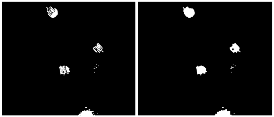
After determining a background image, it is used for background subtraction. Each image frame is subtracted with the background, which preserves the pixels associated with the robot motion, plus some noise due mainly to illumination changes. Figure 6 illustrates a background model and a result of an image frame after background subtraction.

Figure 6.

Left: background model; right: result of background subtraction. In the result, white pixels belong to the foreground (i.e. moving robots) and noise, whereas black pixels belong to the background.

To improve the quality of background subtraction, morphological operations (MOs) are used to eliminate noise and fill the holes in the potential foreground regions. The MOs include erosion (removing small isolated noise) and dilation (filling small holes in the foreground). Example results are shown in Figure 7.

Figure 7.

Left: erosion result on the background subtraction; right: dilation after erosion.

The MO steps ensure that the foreground targets are detected and each component is fully connected. Next, a connected component algorithm finds each region for ROI extraction.

Empirically, one robot occupies a certain range of pixels. Therefore, if a detected region is too small, we can discard it immediately. If two or more robots are merged together, the connected region will be much larger. In this case, multiple targets in one connected region can be easily detected and situation awareness denotes more than one robot. To aid in the ROI extraction, numerous marker designs were evaluated.

Marker design

To design effective markers used in the demonstrator, the following issues were considered:

Distinctness. The markers should be distinct from the surrounding background. In addition, markers for different robots should be able to be distinguished from each other.

Robustness. The markers should be salient against possible illumination, change, and camera projection variations (e.g. distortion when a robot is around the field boundary).

Efficiency. The markers should improve the speed of the orientation estimation.

Many template markers with different styles were constructed and experimentally evaluated. Some templates are shown in Figure 8. The final selections are shown in Figure 8(f)–(h) for three different robots. The main reasons for the selection are as follows: (1) the different block patterns distinguish the three markers; (2) black/white patterns are more stable under illumination changes; and (3) the long stripes provide dominant orientation cues for fast orientation estimation.

Figure 8.

Templates investigate.

In particular, Figure 8(a) shows the original robot, of which a template matching method could be used. However, its structure is hardly perceivable and it will be very time consuming to find the correct alignment. In Figure 8(b), (c), and (e), we introduce colors, but the colors are not robust to illumination changes. Many times, there were color drifting and overlapping threshold bands. Marker in Figure 8(d) is purely a binary template which affords simple template matching. But for a binary marker the search could be tremendously large and deemed to be slow for the PE game. In the end, markers in Figure 8(f)–(h) with the auxiliary stripe lines are used to detect the gradients, thus providing the quick and robust direction and orientation estimation.

Figure 9 shows several examples of the designed markers captured in real sequences. It shows that, given the current imaging condition and image quality, the chosen markers provide the most stable detection over environmental variations.

Figure 9.

Examples of the captured images of different markers.

Orientation estimation

Given the estimated ROIs, a template matching approach searches for the robots and their estimated poses. The first step is to estimate the robot orientation. The search range is a critical issue which has to be carefully examined. Typically, for template matching, a search is conducted along two dimensions of position and one dimension of direction. In the demonstrator project, there are at most three robots to be detected, and thus, for a typical size of 30 × 30 candidate region and a search step of 5 degrees which yields 360/5 = 72 directions, the demonstrator needs 3 × 30 × 30 × 72 = 194,400 searches for only one region.

The search method may take many seconds to process only one frame. But, with the help of the auxiliary line markers which have strong edge features to calculate the edge direction, the search is narrowed down from 72 iterations to only 2 and no more than 10 iterations if a finer direction is needed.

For each detected ROI, the gradient of each pixel along its x and y directions results in the pixel direction using

θ (x, y) = atan (\frac{\partial I (x, y)}{\partial y}, \frac{\partial I (x, y)}{\partial x})

(2)

Notice that there is still a ± π ambiguity because the robot can move forward or backward even at the same location. The problem will be solved by orientation solutions using the two opposite directions (both are needed to calculate the correct direction). By testing both opposite directions, the problem can be overcome through the track history.

Figure 10 shows some examples of the orientation results. For a typical one region target, for example, Figure 10(a), one peak is evident in the cumulative histogram of each pixel direction. Ideally, this peak corresponds to the correct direction or the opposite, that is, correct direction plus π degree. Even if the region contains several candidates, the gradient detection approach could always detect all the directions. As shown in Figure 10(b), the first three peaks correspond to the three robot directions. Notice that the histogram shows the detected gradient direction, and thus another π/2 needs to be added to obtain the correct robot direction.

Figure 10.

Histogram-based robot orientation estimation.

Template matching

After determining the orientation, template matching locates the robot position. For each candidate region, the image is rotated according to the detected direction (pose). Then, to reduce noise, thresholding finds the white and black regions of the target. The thresholds are set empirically and based on the red-green-blue (RGB) and hue-saturation-intensity (HSI) color spaces. As shown in Figure 11, on the right-hand side is the thresholded image, where white regions are white areas in the original image, gray regions are the black regions in the original image, and the black regions are the background.

Figure 11.

Region of interest after color thresholding. Left: original image in grayscale; right: after thresholding, where white pixels indicate the white area in the original image, gray pixels correspond to the black regions in the original image, and black pixels are the background.

The thresholded image is compared with the template images at each position and two orientations to find the best match score. The score is computed as

score (x, y) = {\begin{matrix} 1, if template (x, y) = threshImage (x, y) \\ 0, otherwise \end{matrix}

(3)

score of a region = \sum_{x, y} score (x, y) * mask (x, y)

(4)

where mask(x, y) indicates whether the pixel is foreground or background. Finally, the parameters with the best score are selected as the detected result for the robot positions in the PE game.

To improve the performance in speed and robustness, we introduced several strategies described as follows.

Branch pruning

The naive solution for target detection is through brute force sliding-window search, which is very time consuming. Notice that, during searching, the best candidate so far can actually provide an upper bound for the rest to-be-explored candidates, and this can be used to quickly discard many false candidates.

Specifically, when exploring a new candidate C, if the number of foreground pixels in C is smaller than the best score so far, then C is guaranteed to be worse than the best one so far and therefore can be discarded immediately. By this strategy, a large amount of candidates can be discarded after calculating the number of internal foreground pixels, which, using the integral image, can be calculated extremely fast (in constant time). In our MATLAB experiments, we observed a speedup of about eight times with branch pruning.

Temporal constraints

Although the low frame rate renders the temporal information unreliable, such information, if used properly, may help reduce the potential ambiguity in appearance-based target detection. For this purpose, we integrate temporal information to the detection score of the candidate. Specifically, for a candidate X at frame t, its score to be from template T composes three parts as follows

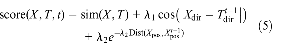
\begin{matrix} score (X, T, t) = & sim (X, T) + λ_{1} \cos (| X_{dir} - T_{dir}^{t - 1} |) \\ + λ_{2} e^{- λ_{2} Dist (X_{pos}, X_{pos}^{t - 1})} \end{matrix}

(5)

where the first term sim(X, T) indicates the similarity between X and T, the second term measures the orientation change of X across time, and the third term captures the position change over time. The temporal constraint is controlled in the second and third terms, weighted by λ₁ and λ₂.

Association constraints

Despite using different templates for three different robots, it can still be very challenging to distinguish them apart under certain conditions, for example, when they cluttered together. To alleviate this issue, we emphasize one-to-one association between candidates and templates. For example, Figure 12 shows the similarity matrix between the three targets and three templates; without the constraint, we will have both targets 2 and 3 matching template 1, which is incorrect in our task. With the constraint, we can correctly match the three pairs of association. Figure 13 shows a real tracking example which shows the effect of the proposed constraints.

Figure 12.

Association constraints. Left: three targets and three templates, where the same color indicates the association with one-to-one constraints; right: the similarity matrix.

Figure 13.

Improvement by temporal and association constraints. Top row: results without applying these constraints on three consecutive frames. An error starts from the second frame. Bottom row: the problem is fixed with the constraints.

Implementation and evaluation

For testing and integration, the algorithms are implemented using mixed MATLAB and C. MATLAB is used for the interface with the PE game, and C is used for the position and orientation searching (using mex files as interfaces). In the basic version, it runs at 0.5 frames per second. A pruning method reduces the search range using the current best score as the heuristic function. The combined efforts achieved a 0.2 s/frame robot position update.

For evaluation, the tracking algorithm is tested on two sequences, named sequence 1 (S1) with 58 frames and sequence 2 (S2) with 259 frames. In most frames, the algorithm achieves excellent results and the estimated orientations are accurate (within about 3 degrees). By visually checking the results on each frame, the calculated accuracies on the two sequences are 100% on S1 and 95.36% on S2.

One example tracking result is shown in Figure 14. Figure 15 shows a typical tracking error. Even in all failed examples, the position estimation is correct, where the errors are mainly attributed to robot identification and orientation inaccuracy. The major failure happens when one or more robots are close to the field boundary, which causes partial occlusion and/or distortion of robot appearances. In addition, the noise level around the image boundary is also higher than that in the interior region.

Figure 14.

The tracking result on one frame. Top left: original image; top right: after background subtraction and post-processing; bottom left: tracking results; bottom right: trajectory to the current frame.

Figure 15.

Incorrect tracking result. Most tracking errors occur when one or more robots are close to the field boundary, or are partly occluded.

Robot dynamics and PE game–based robot controls

Robot dynamics

The robots support three types of commands:

Moving. “Mabc,” where M (with ASCII code 4D) is the command type, a is the left speed, 0x00 through 0x7F is forward, 0xFF through 0x80 is backward, b is for the right speed, c is the duration/10 ms, duration of 00 is infinite. For example, 4D32CF14 means M 50 −50 20, that is, rotate right for 200 ms. 4D000000 is a stop command.

Laser. “L” (4C) to turn off the laser and “l” (6C) to turn on the laser.

Camera. “a” sets the capture resolution to 160 × 120, “b” sets the capture resolution to 320 × 240, “c” sets the capture resolution to 640 × 480, and “d” or “A” sets the capture resolution to 1280 × 1024.

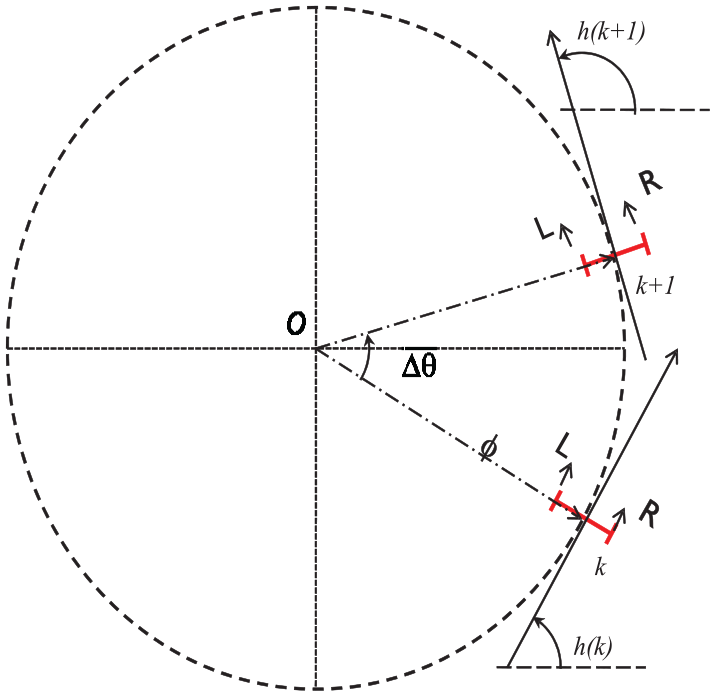
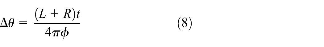
Ideally, each moving command will guide a robot along with a circle (Figure 16). Generally, the radius (ϕ) depends on the left (L)–right (R) speed ratio, Δθ decided by ϕ, command duration (t), and robot average speed, (L + R)/2. The circle center, O, is determined by robot position, robot heading, and ϕ.

Figure 16.

The circular moving feature of the robots.

Usually, the actual speed is different from the commanded speed. That is, L_A = f_L(L_C), where L_C is the commanded left speed and L_A is the actual left speed. Similarly, R_A = f_R(R_C), where R_C is the commanded right speed and R_A is the actual right speed. The functions f_L and f_R mainly depend on robot motor battery level and floor information. We specified f_L and f_R as the linear functions

L = f_{L} (L_{C}) = m L_{A} + n

(6)

R = f_{R} (R_{C}) = p R_{A} + q

(7)

where m and p are the weighted functions to control speed and n and q are the noise. The relations between robot position (x, y), robot heading (h), and moving command (L_A, R_A, t) are illustrated in Figure 17.

Figure 17.

Geometry relations between robot position, robot heading, and robot commands.

Specifically, the robot dynamics are

Δ θ = \frac{(L + R) t}{4 π ϕ}

(8)

h (k + 1) = h (k) + Δ θ

(9)

O_{x} = x (k) + ϕ \cos [h (k) + \frac{π}{2}]

(10)

O_{y} = y (k) + ϕ \sin [h (k) + \frac{π}{2}]

(11)

\begin{matrix} [\begin{matrix} x (k + 1) \\ y (k + 1) \end{matrix}] = [\begin{matrix} \cos (Δ θ) & - \sin (Δ θ) \\ \sin (Δ θ) & \cos (Δ θ) \end{matrix}] \\ [\begin{matrix} x (k) - O_{x} \\ y (k) - O_{y} \end{matrix}] + [\begin{matrix} O_{x} \\ O_{y} \end{matrix}] \end{matrix}

(12)

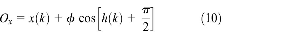
where (O_x, O_y) is the location of the circle center, [x(k), y(k)] is the position of the robot at time k, and h(k) is the robot heading at time k.

General PE game formulation

Based on the robot dynamics in equations (3)–(9), we develop a two-player discrete-time PE game model

X_{P} (k + 1) = X_{P} (k) + A_{P} (h_{P} (k), c_{P} (k))

(13)

h_{P} (k + 1) = h_{P} (k) + H_{P} (c_{P} (k))

(14)

X_{E} (k + 1) = X_{E} (k) + A_{E} (h_{E} (k), c_{E} (k))

(15)

h_{E} (k + 1) = h_{E} (k) + H_{E} (c_{E} (k))

(16)

J_{P} (k) = \min (D (k + 1), r^{1} D (k + 2), \dots, r^{n - 1} D (k + n))

(17)

\begin{matrix} J_{E} (k) = & \min (- D (k + 1), - r^{- 1} D (k + 2), \dots, \\ - r^{- n + 1} D (k + n)) \end{matrix}

(18)

{c_{P} * (k), \dots, c_{P} * (k + n)} = argmin J_{P} (k)

(19)

{c_{E} * (k), \dots, c_{E} * (k + n)} = argmin J_{E} (k)

(20)

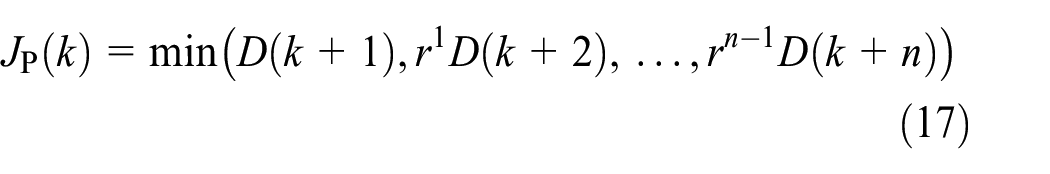
where X_P(k) = [x_P(k), y_P(k)]^T and h_P(k) are the position and heading of the pursuer robot at time k, respectively; A_P and H_P are the nonlinear system dynamics for the position and heading of the pursuer (P) robot, respectively; and c_P(k) is the pursuer robot command at time k. The definitions are similar for equations (15) and (16) for the evader (E).

D(k) is the distance between the pursuer and evader, that is, $D (k) = ‖ X_{P} (k) - X_{E} (k) ‖ \cdot n$ is the planning horizon and r > 1 is the discount factor, which is included here to model the fact that the future performance is less important than the current one. Therefore, the pursuer’s objective function defined in equation (17) is the minimal distance of the n steps. Similarly, the objective of the evader is the maximum of the n distance, that is, the minimum of the n negative distances defined in equation (18). The optimal action sets of n steps are computed from equations (19) and (20). Only the first step will be applied because after that a new game will be constructed with new system states (positions and headings of robots) from the new measurements from the overhead view camera and the visual tracking algorithms.

Limited action space and planning horizon

Generally, A_P, H_P, A_E, and H_E are nonlinear and complicated functions. In this article, only the limited action space cases are investigated, where c_P(k) and c_E(k) can only be chosen from a nine-command set as shown in Figure 18.

Forward: M 50 50 30, moving forward for 300 ms;

Backward: M −50 −50 30, moving backward for 0.3 s;

Right turn: M 70 30 30, right turn for 300 ms;

Left turn: M 30 70 30, left turn for 300 ms;

Back left: M −30 −70 30, back left turn for 300 ms;

Back right: M −70 −30 30, back right turn for 300 ms;

Change heading only, clockwise (CW): M 64 −64 30;

Change heading only, counterclockwise (CCW): M −64 64 30;

Stop (no action): M 0 0 30.

Figure 18.

A limited action space for robots.

A table will be created to store the effects of the nine commands which are called in the control functions. The command effect (Figure 19) is defined as (Δx, Δy, Δh), where (Δx, Δy) is the position change in the local coordinate of a robot and Δh is the heading change, which is the same in the global and local coordinate systems.

Figure 19.

The illustration of the command effects.

A tool was developed to learn the effects of the commands. The basic procedure of the estimator is as follows:

Record the current (x₀, y₀, h₀) of a robot using the tracking algorithm from the overhead image.

Send a command to the robot.

Obtain the position and heading of the robot through the tracking algorithm (x₁, y₁, h₁).

Calculate (Δx₁, Δy₁, Δh₁), where Δh₁ = h₁ – h₀ and

[\begin{matrix} Δ x_{1} \\ Δ y_{1} \end{matrix}] = [\begin{matrix} \cos h_{0} & \sin h_{0} \\ - \sin h_{0} & \cos h_{0} \end{matrix}] [\begin{matrix} x_{1} - x_{0} \\ y_{1} - y_{0} \end{matrix}]

Send an opposite command to the robot. Here the “opposite” operator defined as opposite(M a b c) = M –a –b c.

Obtain the position and heading of the robot through the tracking algorithm (x₂, y₂, h₂).

Calculate (Δx₂, Δy₂, Δh₂), where Δh₂ = h₂ – h₁ and

[\begin{matrix} Δ x_{2} \\ Δ y_{2} \end{matrix}] = [\begin{matrix} \cos h_{1} & \sin h_{1} \\ - \sin h_{1} & \cos h_{1} \end{matrix}] [\begin{matrix} x_{2} - x_{1} \\ y_{2} - y_{1} \end{matrix}]

Repeat steps (a)–(g) for m times.

Computer the averages of (Δx₁, Δy₁, and Δh₁) and (Δx₂, Δy₂, and Δh₂).

Note that two opposite commands are estimated at a time to make sure that the robot will not go outside of the camera view. Table 1 provides the pursuer and evader robots’ calculated geometries of the robot commands.

Table 1.

Robot command effects of the pursuer and the evader.

Commands	Effects of the pursuer robot			Effects of the evader robot
	Δx (pixel)	Δy (pixel)	Δh (rad)	Δx (pixel)	Δy (pixel)	Δh (rad)
M 50 50 30	27.3413	0.9204	0.0025	19.6783	1.6466	0.0674
M 70 30 30	24.2671	0.0959	−0.1181	18.3379	0.5706	−0.0108
M 64 −64 30	2.3673	−5.8313	0.8874	3.3457	−3.9752	0.7130
M −70 −30 30	−25.5022	−4.4570	0.1438	−19.2438	0.0141	0.0496
M −50 −50 30	−28.5634	−2.2056	0.0127	−20.7374	−0.4016	−0.0515
M −30 −70 30	−23.7300	1.3157	−0.1199	−16.5537	3.6019	−0.2797
M −64 64 30	2.8010	5.3365	−0.8673	−1.6785	5.3420	−0.6631
M 30 70 30	24.5951	1.1929	0.1409	17.4523	0.2917	0.2987

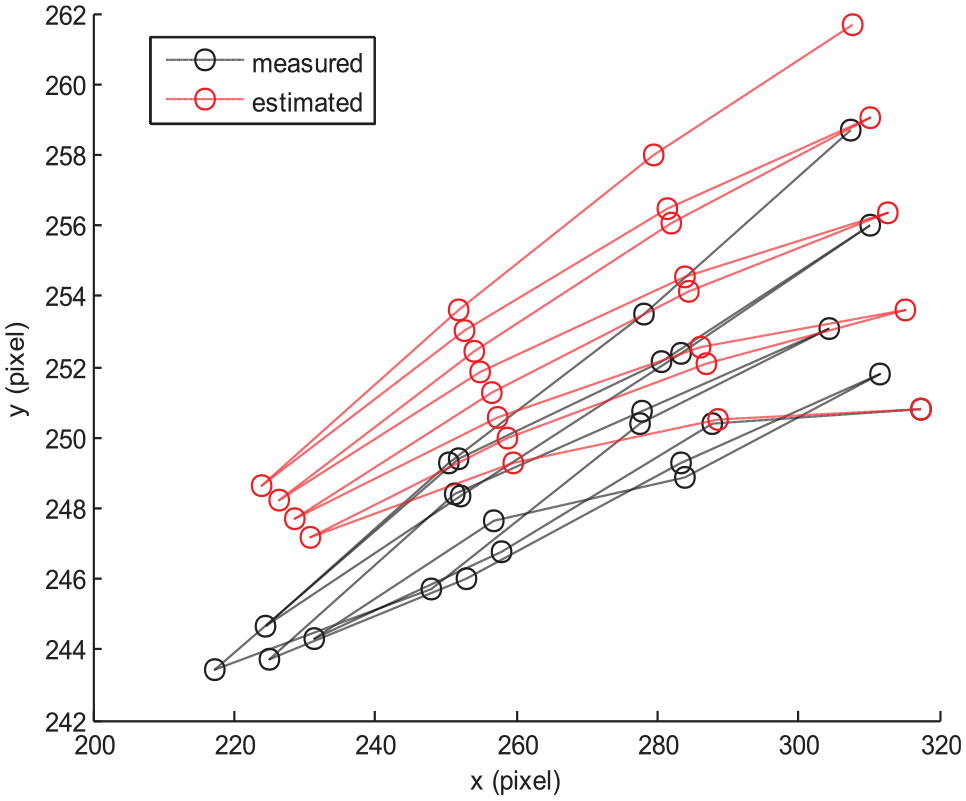
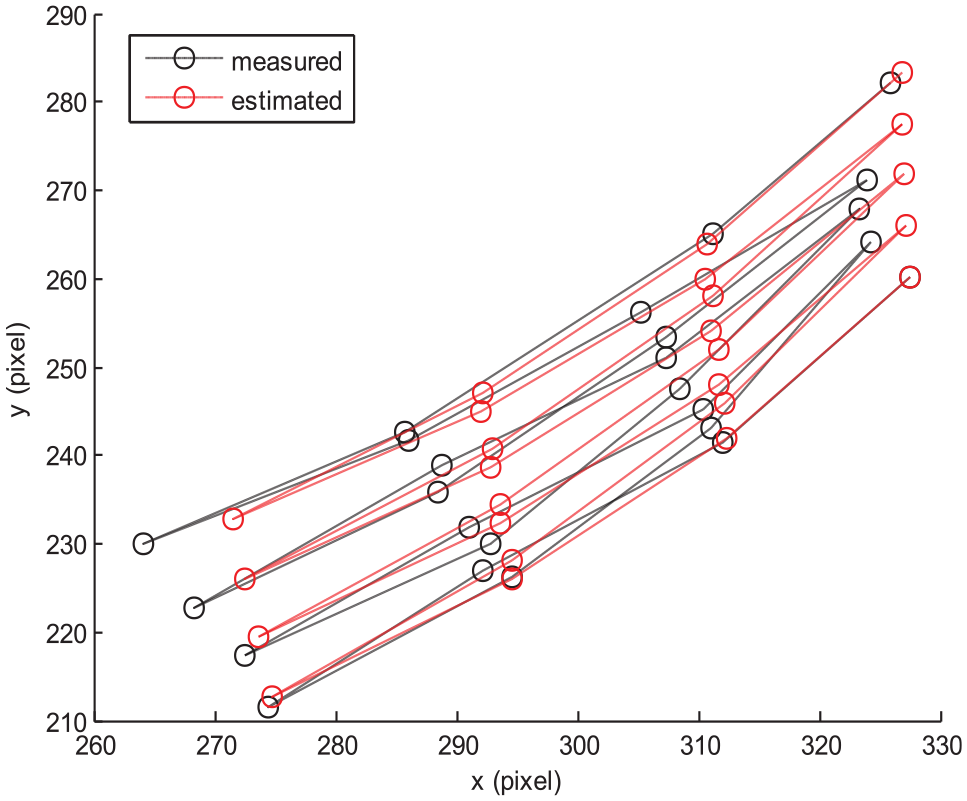
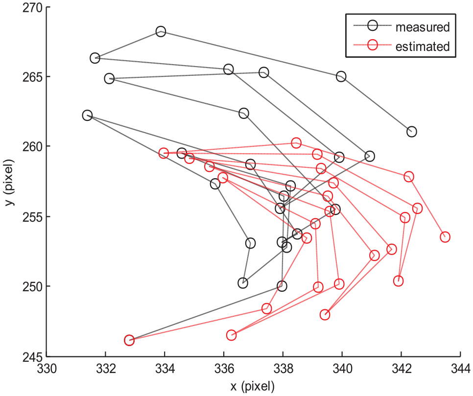
Comparison of the measured and estimated positions of robots in Figures 20 –23 (evader) and Figures 24 –27 (pursuer) demonstrates that the estimated effects are mostly consistent with the measured ones.

Figure 20.

Evaluation of the estimated effects of pursuer’s forward and backward commands.

Figure 21.

Evaluation of the estimated effects of pursuer’s right turn and back right commands.

Figure 22.

Evaluation of the estimated effects of pursuer’s clockwise and counterclockwise commands.

Figure 23.

Evaluation of the estimated effects of pursuer’s left turn and back left commands.

Figure 24.

Evaluation of the estimated effects of evader’s forward and backward commands.

Figure 25.

Evaluation of the estimated effects of evader’s right turn and back right commands.

Figure 26.

Evaluation of the estimated effects of evader’s clockwise and counterclockwise commands.

Figure 27.

Evaluation of the estimated effects of evader’s left turn and back left commands.

For the PE game formulation, given the robot commands in Table 1, the system dynamics are

\begin{matrix} A_{p} (h_{p} (k), c_{p} (k)) = \\ [\begin{matrix} \cos (h_{p} (k)) & - \sin (h_{p} (k)) \\ \sin (h_{p} (k)) & \cos (h_{p} (k)) \end{matrix}] [\begin{matrix} Δ x_{p} (c_{p} (k)) \\ Δ y_{p} (c_{p} (k)) \end{matrix}] \end{matrix}

(21)

h_{P} (k + 1) = h_{P} (k) + Δ h_{P} (c_{P} (k))

(22)

\begin{matrix} A_{e} (h_{e} (k), c_{e} (k)) = \\ [\begin{matrix} \cos (h_{e} (k)) & - \sin (h_{e} (k)) \\ \sin (h_{e} (k)) & \cos (h_{e} (k)) \end{matrix}] [\begin{matrix} Δ x_{e} (c_{e} (k)) \\ Δ y_{e} (c_{e} (k)) \end{matrix}] \end{matrix}

(23)

h_{E} (k + 1) = h_{E} (k) + Δ h_{E} (c_{E} (k))

(24)

where Δx_P(·) and Δy_P(·) are the operators to, based on the robot command, find the Δx and Δy values of the pursuer from Table 1, respectively. Δh_P(·) is the operator to find the Δh value of the pursuer. Similar operators for the evader are Δx_E(·), Δy_E(·), and Δh_E(·).

The geometry meaning of equation (21) or (23) is to transfer the position effects (in the local coordinate system) back to the global coordinate system.

Based on equations (13)–(24), the robot states are propagated from the given initial states. In this article, the planning horizon is set to n = 3, from which the action space of each robot is a set with 9³ = 729 elements. For the 729 × 729 matrix game, results of pure Nash or mixed Nash strategies³ are computed.

Robot demonstration of PE games

MATLAB GUI design

The control interface is implemented using a MATLAB GUI (Figure 28) to integrate all the developed components.

Figure 28.

A MATLAB GUI for the robot simulator.

The plot in the middle is included to show the visual tracking results. In the initialization panel, the robot connection, data structure preparation (including the background modeling), robot initial position configuration, and the automatic pilot are available which can guide the robots to their initial positions.

In extended options, robot dynamics estimation and learning algorithms are provided. Other features include a method to safely disconnect the linked robots.

On the right-hand side of Figure 28, a PE game control panel with the automatic and step-by-step mode options is available. The computed robot controls (commands) are highlighted on the manual control dials, which are also used to select the robot commands during the manual control mode.

Scenario

The scenario for the robot demonstrator is shown in Figure 29, where the initial position of P is at about (158, 184), the initial position of E is at about (189, 394), the boundary is from (50, 100) to (400, 500), and the command effects (Δx, Δy, Δh) of the pursuer and evader are as shown in Table 1. Robots are not allowed to go outside of the boundary.

Figure 29.

A robot scenario for the PE game demonstration.

Results

Figure 30 shows the frame in which the pursuer captured the evader at the right bottom corner. The demo video can be downloaded or viewed from the YouTube link: http://www.youtube.com/watch?v=qZT3BmVSPQ0

Figure 30.

In frame 54, P captured E around a corner.

The trajectories of P and E are shown in Figure 31. As usual, the evader was captured around a corner after 53 steps. The reason is that when the evader is at a corner, E’s feasible action space is reduced due to the constrained boundary.

Figure 31.

The trajectories of the pursuer and evader. Blue circles are for the pursuer and the bar indicates the heading of the robot. Red color is for the evader.

Conclusion

In this article, we designed and implemented a hardware-in-loop PE game-theoretic control framework, which includes the following components: robot dynamic models, PE game models, solutions, entity tracking algorithms, sensor fusion methods, and a PE game demonstration for two robots (one pursuer and one evader). For visual tracking, we designed several markers and selected the one with the best balance of accuracy and robustness. The target robots are detected after background modeling, and the robot pose estimation is from the local gradient patterns. Based on the robot dynamic model, we designed a two-player discrete-time game model with limited action space and limited look-ahead horizons. The robot controls are based on the game-theoretic Nash solutions. We obtained promising results from the hardware-in-loop simulations for the real-time robot PE game-theoretic methods. In the future, we extend our framework to a realistic robot simulator with a flying drone observing, tracking, and following the robots.

Footnotes

Acknowledgements

Thanks to Professor Wei Li of the Department of Computer Engineering and Computer Science, California State University, Bakersfield, CA for the use of the robots for initial validation in the PE game-theoretic robot control framework.

Handling Editor: Eric Fujiwara

Author note

Erik Blasch is now affiliated to Air Force Office of Scientific Research, Arlington, VA, USA.

Declaration of conflicting interests

The author(s) declared no potential conflicts of interest with respect to the research, authorship, and/or publication of this article.

Funding

The author(s) disclosed receipt of the following financial support for the research, authorship, and/or publication of this article: This research was supported by the US Air Force.

ORCID iD

Dan Shen

References

Isaacs

. Differential games: a mathematical theory with applications to warfare and pursuit, control and optimization. New York: John Wiley & Sons, 1965.

Bryson

Jr Baron

. Differential games and optimal pursuit-evasion strategies. IEEE Trans Autom Control 1965; 10: 385–389.

Basar

Olsder

. Dynamic noncooperative game theory. Philadelphia, PA: SIAM, 1998.

Shima

Golan

. Linear quadratic differential games guidance law for dual controlled missiles. IEEE Trans Aerosp Electron Syst 2007; 43: 834–842.

Shaferman

Shima

. Linear quadratic guidance laws for imposing a terminal intercept angle. J Guid Control Dyn 2008; 31: 1400–1412.

Perelman

Shima

Rusnak

. Cooperative differential games strategies for active aircraft protection from a homing missile. J Guid Control Dyn 2011; 34: 761–773.

Parsons

. Pursuit-evasion in a graph. In: Alavi

Lick

(eds) Theory and applications of graphs, vol. 642. New York: Springer, 1976, pp.426–441.

Guibas

Latombe

LaValle

, et al. A visibility-based pursuit-evasion problem. Int J Comput Geomet Appl 1985; 4: 74–123.

Chung

FRK

Cohen

Graham

. Pursuit–evasion games on graphs. J Graph Theor 1988; 12: 159–167.

10.

Adler

Racke

Sivadasan

, et al. Randomized pursuit-evasion in graphs. In: Proceedings of the international colloquium on automata, languages and programming (ICALP), 2002, https://ttic.uchicago.edu/∼harry/pdf/hunter_rabbit_journal.pdf

11.

Wei

Chen

Blasch

, et al. Game theoretic multiple mobile sensor management under adversarial environments. In: Proceedings of the information fusion, 2008, pp.1–8, https://apps.dtic.mil/dtic/tr/fulltext/u2/a520490.pdf

12.

Shen

Chen

Blasch

, et al. Game theoretic sensor management for target tracking. In: Proceedings of the SPIE, vol. 7697, 2010, https://www.researchgate.net/publication/253571618_Game_Theoretic_Sensor_Management_for_Target_Tracking

13.

Isler

Sun

Sastry

. Roadmap based pursuit-evasion and collision avoidance. In: Proceedings of the robotics science and systems, 2005, pp.257–264, http://www.roboticsproceedings.org/rss01/p34.pdf

14.

Shen

Chen

Pham

, et al. Pursuit-evasion orbital game for satellite interception and collision avoidance. In: Proceedings of the SPIE, vol. 8044, 2011, https://www.researchgate.net/publication/253261837_Pursuit-Evasion_Orbital_Game_for_Satellite_Interception_and_Collision_Avoidance

15.

Wei

Chen

Cruz

Jr , et al. Multi-pursuer multi-evader pursuit-evasion games with jamming confrontation. J Aerosp Comput Inform Commun 2007; 4: 676–692.

16.

Wang

Cruz

Jr Chen

, et al. Formation control in multi-player pursuit evasion game with superior evaders. In: Proceedings of the SPIE, vol. 6578, 2007, https://www.researchgate.net/publication/228721681_Formation_control_in_multi-player_pursuit_evasion_game_with_superior_evaders

17.

Cruz

Jr Schumacher

. Stochastic multi-player pursuit–evasion differential games. Int J Robust Nonlin Control 2008; 18: 218–247.

18.

Wei

Chen

Cruz

Jr , et al. A decentralized approach to pursuer-evader games with multiple superior evaders in noisy environments. In: Proceedings of the IEEE aerospace conference, 2007, http://www2.ece.ohio-state.edu/∼cruz/Papers/C131-z06_0302-Mo-1.pdf

19.

Cruz

Jr Chen

, et al. A hierarchical approach to multi-player pursuit-evasion differential games. In: Proceedings of the 44th IEEE European conference on decision and control, Seville, 15 December 2015. New York: IEEE.

20.

Wei

Chen

Cruz

Jr , et al. Game-theoretic modeling and control of military operations with partially emotional civilian players. Decis Support Syst 2008; 44: 565–579.

21.

Cruz

Jr . Information, decision-making and deception in games. Decis Support Syst 2009; 47: 518–527.

22.

Blasch

Bosse

Lambert

. High-level information fusion management and systems design. Norwood, MA: Artech House, 2012.

23.

Surveyor SRV-1 Blackfin robot: open source wireless mobile robot with video for telepresence, autonomous and swarm operations, http://www.robotcombat.com/products/IL-SRV1Q.html

24.

Ling

Blasch

, et al. Evaluation of visual tracking in extremely low frame rate wide area motion imagery. In: Proceedings of the international conference on information fusion, 2011, http://www.dabi.temple.edu/∼hbling/publication/CLIF_tracking_4.pdf

25.

Lee

Zhi

Blenis

, et al. Real-time vision-based tracking control of an unmanned vehicle. J Mechatron Intell Motion Control 1995; 5: 973–991.

26.

Wang

Cheng

, et al. Real-time probabilistic covariance tracking with efficient model update. IEEE Trans Image Process 2012; 21: 2824–2837.

Computer vision and pursuit–evasion game theoretical controls for ground robots

Abstract

Keywords

Introduction

Overall framework and hardware setup

Overall framework

Hardware setup

Visual tracking algorithms

Tracking-by-detection approach

Background modeling and extraction of ROIs

Marker design

Orientation estimation

Template matching

Branch pruning

Temporal constraints

Association constraints

Implementation and evaluation

Robot dynamics and PE game–based robot controls

Robot dynamics

General PE game formulation

Limited action space and planning horizon

Robot demonstration of PE games

MATLAB GUI design

Scenario

Results

Conclusion

Footnotes

Acknowledgements

Author note

Declaration of conflicting interests

Funding

ORCID iD

References