Sage Journals: Discover world-class research

Abstract

A two-dimensional numerical model is developed to investigate the phenomenon of resonance in narrow gaps. Instead of using commonly used Volume of Fluid method to capture the free surface which is sometimes difficult to capture the geometric properties of the geometrically complicated interface, the free surface is traced by using Arbitrary Lagrangian–Eulerian method. The numerical model is based on the two-dimensional Reynolds-Averaged Navier–Stokes equations. The numerical model is validated against wave propagation in wave flume. Comparisons between the numerical results and available theoretical data show satisfactory agreements. Fluid resonance in narrow gaps of fixed rectangular structures are simulated. Numerical results show that resonance wave height and wave frequency for rectangle boxes with sphenoid corners is larger than for rectangle boxes.

Keywords

Water wave narrow gaps Arbitrary Lagrangian–Eulerian resonance viscous numerical model

Introduction

Gap resonance phenomena may happen when two or multiple floating structures are installed in side-by-side form with narrow gaps which are subjected to waves. Vertical oscillation amplitude of fluid in the narrow gap between may be much larger than the incident wave height. Large amplitude will lead to extreme wave forces on structures, which is dangerous to the structures. The phenomenon of resonance in narrow gap has received more and more attention in marine activity due to the potential threat to the structures.

There are mainly three methods to investigate the gap resonance problem: (1) theoretical and experimental analysis methods, (2) potential flow numerical analysis, and (3) viscous flow numerical analysis method. The natural modes of oscillation of the inner free surfaces in moon pools are determined by Molin et al.¹ under the assumption of infinite water depth and infinite length and beam of the barges that contain the moon pools. Simple quasi-analytical approximations for resonance frequency in the gap were derived. Saitoh et al.² theoretically presented an appearance condition of resonance phenomena in a narrow gap between two modules of very large floating structures in waves by using the conservation of energy. An assumption that flow in the gap and around the module of the incident wave side is the same as flow motion in a two-dimensional (2D) U-tube with different diameters was adopted. A laboratory experiment is also conducted by Saitoh et al.² in order to verify the appearance condition that was obtained from theoretical method. The maximum wave height in the gap could reach to over five times of the incident wave height when the resonance occurred in the laboratory experiment. Iwata et al.³ extended the theoretical analysis and the experiment of Saitoh et al.² to two-gaps cases composed of three rectangular modules. Gap resonance phenomena also been observed for the case of two gaps. In addition, the resonant wave number shifted to lower frequency as the draft and the gap width increased. The second resonant mode is found for the gap in the incident wave side. Zhao et al.⁴ investigated first and higher harmonic components of the resonant fluid response in the gap between two identical fixed rectangular boxes in a wave basin. NewWave analysis and reciprocity were given by Zhao et al.⁵

There are also many researchers who studied the problem of gap resonance by using numerical simulation method, and most of them are using potential flow numerical analysis method. Miao et al.⁶ studied the wave interaction of twin fixed caissons with rectangular sections with a small gap. A sharp peak force response on each caisson was proved due to the narrow resonant phenomena. Moreover, the resonant phenomena occur around kL = nπ(n = 1, 2, 3, …, ∞) which is called the resonant wave number, where k is the incident wave number and L is characteristic length of the structure. Zhu et al.⁷ developed a three-dimensional (3D) time domain method to investigate the gap influence on the wave forces for 3D multiple floating structures based on potential flow assumption. However, it has been generally accepted that the models based on conventional potential flow theory over-predict the wave height in the narrow gap because of no flow viscous, no energy dispassion considered. Some attempts have been made to overcome the disadvantage of potential flow models. Lu et al.⁸ studied the problem of fluid resonance in narrow gaps by using potential flow model with artificial damping force and found that the accuracy of the predicted resonant wave height in narrow gaps can be improved greatly by introducing appropriate damping force into the potential flow model. The most interesting result was that the damping coefficient used for the potential flow model is not sensitive to the geometric dimensions and spatial arrangement. Sun et al.⁹ used a second-order diffraction calculation, based on a quadratic boundary element method, to examine the behavior of two parallel closely spaced rectangular barges.

It should be noted that although the potential flow model can predict the resonance wave height in the gap in good agreement with the laboratory data by adding artificial damping force, the introduction of the damping coefficient is empirical. Therefore, using Computational Fluid Dynamics (CFD) method based on viscous flow has advantage to study the fluid resonance in narrow gaps. Lu et al.¹⁰ developed a CFD model based on the finite element solution of Navier–Stokes equations. To capture the free surface, the CLEAR–Volume of Fluid (CLEAR-VOF) method is used. And waves are generated by using the internal wave maker method. Problem of fluid resonance in two narrow gaps of three identical rectangular structures was investigated by Lu et al.¹⁰ using the developed CFD numerical model. It was found that the fluid resonance occurred in both of the narrow gaps at distinct frequencies. Moradi et al.¹¹ investigated the effect of inlet configuration on wave resonance in the narrow gap of two fixed bodies in close proximity by using a CFD numerical model built on the Open FOAM platform. The maximum wave height in the gap could reach about 11 time of the incident wave height for the two fixed rectangle structures with round corner. Most of the CFD models use the VOF method to capture the water free surface. And although the VOF method has been proved to predict the fluid resonance well, it is very difficult to capture the geometric properties of the geometrically complicated interface sometimes by using VOF method. Therefore, it is necessary to develop a CFD model without considering the geometric properties.

The aim of this study is to establish a 2D viscous numerical model to simulate fluid resonance in narrow gaps by using Arbitrary Lagrangian–Eulerian (ALE) method. This numerical model is an extension of the previous model proposed by Zhao and Cheng¹² and Liu et al.¹³ This article is organized as follows. The details of the numerical model will be described in the “Numerical models” section, followed by necessary numerical validations in the “Numerical validations” section. Numerical results of fluid resonance in narrow gaps will be presented in the “Resonance between two fixed rectangle boxes with sphenoid corners” section. Finally, conclusions will be drawn in the “Conclusion” section.

Numerical models

Governing equations

The governing equations for incompressible viscous Newtonian fluid with free surface are the 2D Reynolds-Averaged Navier–Stokes (RANS) equations, which can be written as follows

\frac{\partial u_{i}}{\partial x_{i}} = 0

(1)

\frac{\partial u_{i}}{\partial t} + (u_{j} - u_{j}^{m}) \frac{\partial u_{i}}{\partial x_{j}} = - \frac{1}{ρ} \frac{\partial p}{\partial x_{i}} + ν \frac{\partial}{\partial x_{j}} (\frac{\partial u_{i}}{\partial x_{j}}) + g_{i}

(2)

where u_i is the ith velocity component corresponding to x_i by using the Cartesian coordinates (u₁ = u and u₂ = v for x₁ = x and x₂ = y, respectively), $u_{j}^{m}$ is the velocity of the motion of the grid, t is the time, p is the pressure, ρ is the fluid density, ν is the kinematic viscosity, g_i denotes the acceleration (g₁ = 0.0 and g₂ = g where g is the gravitational acceleration).

In the present numerical model, the wave free surface is traced by using ALE method which is different from the previous research, most of which use the VOF method to capture the free surface which is sometimes difficult to capture the geometric properties of the geometrically complicated interface.

The governing equation for the displacements of the mesh nodes is the modified Laplace equation¹⁴

\nabla \cdot (γ \nabla S_{i}) = 0

(3)

where S_i represents the displacement of the mesh nodal point in the x_i direction, and γ is a control parameter used to guarantee the mesh quality, avoiding excessive deformation, near the structure and the free surface, where dense mesh is used. In the present numerical model, the parameter γ is set to be γ = 1/A with A being the area of the finite element.

The governing equations are solved by using the Streamline Upwind Petrov–Galerkin (SUPG) finite element method, which has been successfully used in simulating the motion of fluid by Liu et al.¹³ and Zhao et al.¹⁵

Computational domain and boundary conditions

A definition sketch for wave propagation over two adjacent fixed rectangle boxes with sphenoid corners in this work is shown in Figure 1. Two adjacent fixed rectangle boxes with sphenoid corners are placed in the center of a numerical wave flume with length equals 20 m and depth h = 0.5 m. The draft of the two boxes is d = 0.25 m. The length of the sphenoid corners is defined as R. The width of the narrow gap between the two boxes is kept at a constant B_g = 0.05 m.

Figure 1.

Computational domain for wave propagation over two adjacent fixed rectangle boxes with sphenoid corners.

At the inlet, ∂p/∂x = 0 is applied for the pressure. The velocity components and the wave elevation are imposed according to a linear wave theory as follows

U (y, t) = \frac{H ω}{2} \frac{\cosh k (y + h)}{\sinh kh} \cos (ω t)

(4)

V (y, t) = - \frac{H ω}{2} \frac{\sinh k (y + h)}{\sinh kh} \sin (ω t)

(5)

η (t) = \frac{H}{2} \cos (ω t)

(6)

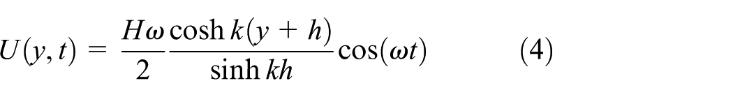
where U and V are the inlet velocity in x and y direction, respectively. And H is wave height, ω is the circular frequency of the wave, η is the elevation of the free surface, k is wave number which can be obtained from the following dispersion relation

ω^{2} = gk \tanh kh

(7)

For the outlet boundary, the Sommerfeld radiation condition is applied for all physical variables, that is

\frac{\partial φ}{\partial t} + α \frac{\partial φ}{\partial x} = 0

(8)

where φ denotes any physical variable and α is the wave celerity.

In order to eliminate the reflected wave, relaxation zones are implemented in front of both ends of the computational domain. In the relaxation zones

ψ = α_{R} ψ_{computed} + (1 - α_{R}) ψ_{target}

(9)

where ψ is the velocity or the free surface. The coefficient α_R can be calculated from the following equation

α_{R} = 1 - \frac{e^{x_{R}^{3.5}} - 1}{e - 1} for x_{R} \in [0, 1]

(10)

where x_R is the non-dimensional distance from the computational domain to the inlet/outlet boundary. Details for x_R and α_R can be obtained from Figure 2. In this study, 4.0 m long relaxation zones are adopted in front of both the inlet and the outlet boundary.

Figure 2.

Sketch of the variation of x_R and α_R for both inlet and outlet relaxation zones.

For the bed boundary, no-slip boundary is adopted, ∂p/∂x = 0 is applied for the pressure. The velocity components are set to be 0.

The governing equation for the free surface profile can be written as the following according to the fully nonlinear kinematic boundary condition¹³

\frac{\partial η}{\partial t} + (u_{1} - u_{1}^{m}) \frac{\partial η}{\partial x_{1}} = u_{2}

(11)

For the structure surface boundary, no-slip boundary is adopted, ∂p/∂x = 0 is applied for the pressure. The velocity components are set to be 0.

At the waterline, the flow velocity is forced to be the same as the velocity of the first layer of mesh node around the structure.

Numerical validations

Wave propagation

In order to illustrate that present numerical model can be used to simulate the problem of wave propagation, a typical linear wave with wave height H = 0.01 m, wave period T = 3.2 s, and water depth d = 1.0 m is generated in a 30 m long numerical wave tank. Figure 3 shows time history of wave free surface at x = 10 m. It can be seen from Figure 3 that present numerical results tally very well with the theoretical solutions. Figure 4 gives the wave free surface in the wave after 80 T. The good comparisons between the result of present numerical model and theoretical solutions demonstrate that present numerical model can be used to simulate the problem of linear wave propagation in wave tank.

Figure 3.

Time history of wave free surface at x = 10 m.

Figure 4.

Wave free surface in the wave after 80 T.

Performance of relaxation zones

The performance of the relaxation zone is examined by simulating the problem of wave propagation before a wall. In the simulation, a linear wave with water depth d = 0.5 m, wave period T = 1.2 s, and wave height H = 0.04 m is generated in a 20 m long wave tank with a wall in the end as shown in Figure 5.

Figure 5.

Sketch and definition of wave propagation before a wall.

Figure 6 gives time history of wave free surface at x = 0.0 m. It can be seen from Figure 6 that before about t = 20 s, the wave height at x = 0.0 m almost equals the incident wave height which is 0.04 m, the wave height increases to about 0.08 m gradually from about t = 20 to 30 s. After 40 s, the wave height at x = 0.0 m keeps 0.08 m steady which is twice of the incident wave height. The wave profile in the wave tank is given in Figure 7 at t = 65 and 65.5 T. It can be seen from Figure 7 that on the inlet boundary, the wave height is equal to the incident wave height H = 0.04 m and out of the relaxation zone, the wave height is twice that of incident wave height. Therefore, the relaxation zone works very well in removing secondary reflection for the problem of the interaction between wave and structures.

Figure 6.

Time history of wave free surface at x = 0.0 m.

Figure 7.

Wave profile in the wave tank.

Resonance in narrow gap

It can be seen that the present numerical model works well in simulating the propagation of wave and can remove the secondary reflection effectively from the previous discussion. In this part, the problem of resonance in narrow gap between two fixed rectangle boxes is simulated. In the simulation, the width of the boxes is B = 0.5 and the width of the gap is B_g = 0.005 m, the water depth is h = 0.5 m, the draft is d = 0.25 m, and the incident wave height is H₀ = 0.024 m. The details of the sketch and definition can be found in Figure 8.

Figure 8.

Sketch and definition of computation.

The dependence of the non-dimensional wave height H_g/H₀ in the narrow gap at x = 0.0 m with kh is presented in Figure 9. To validate the present numerical model, the experimental data of Saitoh et al.² is also included in Figure 9. From the comparison of present numerical results and the laboratory results of Saitoh et al.,² it can be seen that the present numerical results agree very well with the experimental data both in the resonance frequency and the resonance wave height. Therefore, the present numerical model can be used to simulate the problem of resonance in narrow gap.

Figure 9.

Comparison of the variations of non-dimensional wave height with incident wave frequency in the gap.

Resonance between two fixed rectangle boxes with sphenoid corners

In this section, the phenomenon of resonance between two fixed rectangle boxes with sphenoid corner is investigated. Two rectangle boxes with sphenoid corner are fixed in a 20 m long wave flume. The width of the boxes is B = 0.5 m, the water depth is h = 0.5 m, the draft d = 0.25 m, and the width of the gap is B_g = 0.05 m. The details of the setup of the simulation can be clearly seen in Figure 1.

Figure 10 shows the variation of non-dimensional wave height with incident wave frequency in the gap under R = 0.0 m and R = 0.025 m. It can be seen that the maximum wave height in the gap for R = 0.025 m, which is about 8.0 times that of incident wave height, is much larger than that R = 0.0 m. Moreover, the resonance frequency for R = 0.025 m moves to about kh = 1.59 which is larger than that of R = 0.0 m, the resonance frequency of which is about kh = 1.53. Therefore, the resonance wave height and wave frequency are larger for rectangle boxes with sphenoid corners compared with two rectangle boxes.

Figure 10.

Comparison of the variations of non-dimensional wave height with incident wave frequency in the gap.

Figure 11 shows effect of R on wave height in the gap. The resonance frequencies become larger with increase of R. However, the resonance wave height changes little. This may be because the increase of R makes mass participating in resonance larger.

Figure 11.

Effect of R on wave height in the gap.

Figure 12 gives the comparison of wave height in the gap between three rectangle boxes and three boxes with sphenoid shape corner and R = 0.025 m. As there are three boxes, two gaps are formed. Figure 12(a) gives the wave height in the front gap while Figure 12(b) shows the wave height in the rear gap. It can be seen that there are two resonance frequencies in the front gap front Figure 12(a). In addition, wave height in this gap for rectangle boxes with sphenoid corners is larger than rectangle boxes and the resonance frequencies for rectangle boxes with sphenoid corners are larger. From Figure 12(b), it can be seen that different from rectangle boxes, there are two resonance frequencies for rectangle boxes with sphenoid shape corner.

Figure 12.

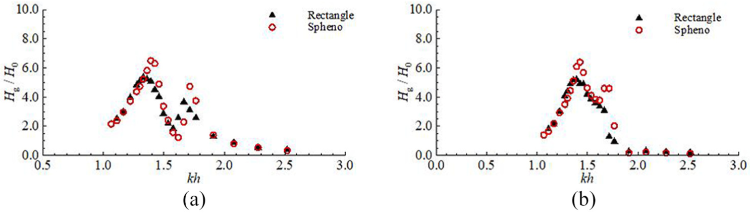
Comparison of wave height in the gap between three boxes: (a) wave height in front gap and (b) wave height in rear gap.

Conclusion

A two-dimensional numerical model was set up to investigate wave resonance between two and three boxes by solving the incompressible Navier–Stokes equations directly. The ALE method is used to trace the free surface of wave. The numerical model validated works well in simulating wave propagation problems. Based on the numerical results, three conclusions are obtained as follows:

Resonance wave height and wave frequency for rectangle boxes with sphenoid corners is larger than for rectangle boxes.

Resonance wave frequencies get larger with increase of R.

For three boxes with two gaps, there is an additional resonance frequency for rectangle boxes with sphenoid corners.

Footnotes

Handling Editor: James Baldwin

Declaration of conflicting interests

The author(s) declared no potential conflicts of interest with respect to the research, authorship, and/or publication of this article.

Funding

The author(s) disclosed receipt of the following financial support for the research, authorship, and/or publication of this article: The authors would like to acknowledge the support from State Key Laboratory of Coastal and Offshore Engineering Projects Program (Grant No. LP1912), the National Natural Science Foundation of China (Grant No. 51809133), and Zhejiang Provincial Natural Science Foundation of China (Grant No. LY16E090002).

ORCID iD

Ming-ming Liu

References

Molin

Remy

Camhi

et al. Experimental and numerical study of the gap resonances in-between two rectangular barges. J Exp Marine Biol Ecol 2009; 30: 2521–2523.

Saitoh

Miao

Ishida

. Theoretical analysis on appearance condition of fluid resonance in a narrow gap between two modules of very large floating structure. In: Proceedings of the third Asia-Pacific workshop on marine hydrodynamics, Shanghai, China, 27–28 June 2006, pp.170–175.

Iwata

Saitoh

Miao

. Fluid resonance in narrow gaps of very large floating structure composed of rectangular modules. In: Proceedings of the fourth international conference on Asian and Pacific coasts, Nanjing, China, 21–24 September 2007, pp.815–826. Beijing, China: China Ocean Press.

Zhao

Wolgamot

Taylor

et al. Gap resonance and higher harmonics driven by focused transient wave groups. J Fluid Mech 2017; 812: 905–939.

Zhao

Taylor

Wolgamot

et al. Linear viscous damping in random wave excited gap resonance at laboratory scale—NewWave analysis and reciprocity. J Fluid Struct 2018; 80: 59–76.

Miao

Saitoh

Ishida

. Water wave interaction of twin large scale caissons with a small gap between. Coast Eng 2001; 43: 39–58.

Zhu

Miao

. A time domain investigation on the hydrodynamic resonance phenomena of 3-D multiple floating structures. J Hydrodyn 2008; 20: 611–616.

Teng

Cheng

et al. Modelling of multi-bodies in close proximity under water waves—fluid resonance in narrow gaps. Sci China 2011; 54: 16–25.

Sun

Eatock Taylor

Taylor

. First- and second-order analysis of resonant waves between adjacent barges. J Fluid Struct 2010; 26: 954–978.

10.

Cheng

Teng

et al. Numerical investigation of fluid resonance in two narrow gaps of three identical rectangular structures. Appl Ocean Res 2010; 32: 177–190.

11.

Moradi

Zhou

Cheng

. Effect of inlet configuration on wave resonance in the narrow gap of two fixed bodies in close proximity. Ocean Eng 2015; 103: 88–102.

12.

Zhao

Cheng

. Numerical investigation of local scour below a vibrating pipeline under steady currents. Coast Eng 2010; 57: 397–406.

13.

Liu

Teng

et al. Numerical modeling of local scour and forces for submarine pipeline under surface waves. Coast Eng 2016; 116: 275–288.

14.

Zhao

Cheng

. Numerical modelling of local scour below a piggyback pipeline in currents. J Hydraul Eng 2008; 134: 1452–1463.

15.

Zhao

Cheng

Teng

et al. Hydrodynamic forces on dual cylinders of different diameters in steady currents. J Fluid Struct 2007; 23: 59–83.

Numerical modeling of fluid resonance in narrow gaps of fixed rectangular structures

Abstract

Keywords

Introduction

Numerical models

Governing equations

Computational domain and boundary conditions

Numerical validations

Wave propagation

Performance of relaxation zones

Resonance in narrow gap

Resonance between two fixed rectangle boxes with sphenoid corners

Conclusion

Footnotes

Declaration of conflicting interests

Funding

ORCID iD

References