Layered manufacturing for medical imaging data

Abstract

Layered manufacturing techniques have been successfully employed to construct scanned objects from three-dimensional medical image data sets. The printed physical models are useful tools for anatomical exploration, surgical planning, teaching, and related medical applications. Before fabricating scanned objects, we have to first build watertight geometrical representations of the target objects from medical image data sets. Many algorithms had been developed to fulfill this duty. However, some of these methods require extra efforts to resolve ambiguity problems and to fix broken surfaces. Other methods cannot generate legitimate models for layered manufacturing. To alleviate these problems, this article presents a modeling procedure to efficiently create geometrical representations of objects from computerized tomography scan and magnetic resonance imaging data sets. The proposed procedure extracts the iso-surface of the target object from the input data set at the first step. Then it converts the iso-surface into a three-dimensional image and filters this three-dimensional image using morphological operators to remove dangling parts and noises. At the next step, a distance field is computed in the three-dimensional image space to approximate the surface of the target object. Then the proposed procedure smooths the distance field to soothe sharp corners and edges of the target object. Finally, a boundary representation is built from the distance field to model the target object. Compared with conventional modeling techniques, the proposed method possesses the following advantages: (1) it reduces human efforts involved in the geometrical modeling process. (2) It can construct both solid and hollow models for the target object, and wall thickness of the hollow models is adjustable. (3) The resultant boundary representation guarantees to form a watertight solid geometry, which is printable using three-dimensional printers. (4) The proposed procedure allows users to tune the precision of the geometrical model to compromise with the available computational resources.

Introduction

Computerized tomography (CT) scan and magnetic resonance imaging (MRI) are powerful technologies for producing cross-sectional images of three-dimensional (3D) objects. They are widely used in medical, biological, archeological, security, and other related applications. ¹ Since these scanning processes produce massive-volume data sets, it is impossible to analyze the results by hand. Instead, MRI and CT-scan data sets are usually explored using computerized graphical techniques to reveal the anatomical and geometrical features of the scanned objects. Among those graphical techniques, slicing, iso-surface extraction, ² and volume rendering ³ are the most popular ones. Although these graphical techniques are useful for visualizing volume data, they generate no physical model. By merely examining the images shown on the computer screen, users may not be able to comprehend the real shapes, sizes, and internal structures of the scanned objects. Furthermore, users could be fooled by the images if too much artificial shading effects were added during the rendering process.

Layered manufacturing (LM) techniques build objects in a layer-by-layer manner. Compared with conventional manufacturing procedures, they are more flexible and cheaper. Thus, LM techniques are getting popular in prototyping and product manufacturing. ⁴ Scientists and engineers had also applied LM techniques in numerous medical applications, including cosmetic surgeries, bone replacement, surgical planning, and tissue and organ model reconstruction. ⁵ LM methods are applicable to the exploration of CT-scan and MRI data too. Users can employ these techniques to generate physical models from the data sets to obtain a better understanding about the scanned objects. However, before printing a physical model, users have to first construct a geometrical representation of the object from the input data set. Subsequently, they can employ a slicer to generate G-codes and use 3D printers to manufacture the physical model. In addition, the study by Turner and Gold ⁶ showed that the quality of the geometrical representation influences the precision of the printed object. Therefore, geometrical modeling is the most essential computation for LM.

Giannopoulos et al. ⁷ presented an innovative LM procedure to create a heart model and a fixation patch, which were used in a remedy operation in an infant’s heart. In the procedure, the researchers used a segmentation software tool to extract the blood pools of the heart and major vessels from the input CT-scan data. Then, they utilized a geometrical modeling program to grow the surfaces of the heart and the major vessels from the blood pools. At the following stage, they employed another computer-aided design (CAD) software to refine the heart model and to create the fixation patch. Finally, the heart model and the fixation patch were converted into G-codes using a slicer and manufactured using 3D printers. Giannopoulos et al. ⁷ verify the tremendous contribution of LM techniques to medical applications. At the mean time, they also reveal the importance and complexity of the geometrical modeling process, embedded in the LM procedure. Numerous human efforts and software tools were employed in the preparation of the heart and patch models. Applying their LM procedure to prototype organs and tissues from CT and MRI data would be a challenge for ordinary users.

Motivated by the works of Turner and Gold ⁶ and Giannopoulos et al., ⁷ we developed a geometrical modeling procedure aiming to reduce the complexity of the modeling process and to increase the efficiency and usability of LM in medical applications. Our geometrical modeling procedure represents the target objects using iso-surfaces (triangular meshes), voxel-based models (3D images), and distance fields (continuous functions) at different stages of the modeling procedure and applies suitable refinement and filtering operators on these geometrical representations to remove noises and abrupt geometrical features. Hence, the geometrical models are gradually improved along with the progression of the modeling process. At the end of the modeling procedure, the final models are extracted and expressed in boundary representations (B-reps) to comply with the requirements of LM processes.

Related work and technical background

The stereolithography (STL) format is the de facto description of geometrical models in LM. In an STL file, the target model is usually represented by triangular facets. These triangular facets form a closed surface which is watertight and encloses a solid geometry. As this surface model is sliced, each resultant slice contains one or multiple disjoint closed two-dimensional (2D) contours. These contours uniquely define the internal and external spaces of the target object, and thus the target object can be printed correctly. However, CT-scan and MRI data sets are recorded in voxel-based formats. Slicers of LM systems cannot process these data sets directly. Hence, specialized geometrical modeling tools, which are capable of generating feasible surface representations from volume data sets, are required to accomplish LM for the scanned objects hidden in CT and MRI data.

Littley and Voiculescu ⁸ proposed a geometrical modeling procedure to build a geometrical representation for a scanned object hidden in a medical image data set. This procedure computes the 2D contours of the target object in all cross-sections of the input volume data at first. Then the surface mesh of the target object is formed by connecting these contours. The resultant surface mesh is a watertight solid geometry and feasible for LM. Their method and other similar approaches ⁹ are widely used for constructing geometric models from CT and MRI data. However, these methods may encounter difficulties if some of the segmented contours are not closed or the numbers of contours of two adjacent cross-sections are different. Thus, extra efforts are required to repair broken surfaces and to resolve ambiguities. Other researchers extracted the iso-surface of the target object from the volume data and treated the iso-surface as the geometrical representation of the target object for LM. ¹⁰ Nonetheless, if this iso-surface model contains holes or dangling parts, it does not form a watertight solid geometry and cannot unambiguously specify the boundary of the target object. Therefore, the slicer of the LM process may fail to produce the correct G-codes ¹¹ to fabricate the target object. Thus, iso-surfaces are not ideal geometrical models for LM. To overcome this problem, the proposed geometrical modeling procedure constitutes a pipeline which gradually refines iso-surface models and produces watertight solid geometries at the end of the modeling process. It can be used to improve the results generated by the modelers similar to that of Wang et al. ¹⁰

Segmentation is an alternative way for creating geometrical models from volume data sets. In a segmentation computation, users create a region of interest in the volume data using thresholding, ¹² region growing, ¹³ diffusion processes, ¹⁴ pattern matching, ¹⁵ clustering, and other techniques. ¹⁶ These segmentation methods efficiently produce voxel-based models from volume data sets. However, conventional slicers cannot convert voxel-based models into G-codes. The segmented results must be transferred into polygon-based representations using additional tools before being processed by slicers and manufactured by 3D printers. The proposed geometrical modeling procedure transforms voxel-based models into smooth distance fields and extracts watertight surface models, acceptable by slicers, from the resultant distance fields. Thus, our modeling procedure can be combined with segmentation programs to build geometric models from medical imaging data.

In the proposed modeling procedure, distance field transformation is the key computation. It requires significant computer resources, and the computed distance field determines the precision of the final B-rep. The fast marching method (FMM), presented by Sethian, ¹⁷ is an efficient algorithm for computing distance fields. This method regards the Eikonal equation as the governing equation of the distance field. It approximates derivatives using an upwind difference method such that the distance information propagates from the boundary toward the remaining space. Then, it calculates the distance field in a point-by-point manner using a downwind updating approach. In each step of the downwind updating process, the point, which is the closest and with unknown distance, is searched at first. Then, the distance of this point is decided using the distances of adjacent points, which have been processed at previous iterations. To speed up the computation, the FMM employs a heap-sort procedure to find the closest point. Another popular approach for building distance fields is the fast sweeping method (FSM). ¹⁸ The FSM also employs Sethian’s ¹⁷ downwind difference method to approximate derivatives and converts the governing equation into an algebraic equation. However, it uses a Gauss–Seidel iteration method to calculate the distance field. In the computation, it assigns an initial distance to the boundary points at first. Then it selects a sweeping direction to update the entire distance field based on an algebraic equation. Once the updating is completed, it choses another sweeping direction to revise the distance field again. By altering the sweeping direction and repeating the updating, this method guarantees that the distance field monotonically converges. Thus, the computation will end at a definite number of iterations. In this work, we deduce a revised FMM to compute distance fields in 3D lattice space. Our method simplifies the computational procedures of Sethian ¹⁷ and Zhao ¹⁸ and is more elegant and easier to implement. Details of the revised FMM are presented in section “Continuous representation generation.”

Overview of the proposed geometrical modeling procedure

The flowchart of the proposed procedure is illustrated in Figure 1. At the first stage, the iso-surface of the target object is extracted from the input volume data using the marching cube method. ² The resultant iso-surface is merely a preliminary geometrical model of the target object. It may be disconnected and contain small holes and gaps. At the second stage, we discretize the iso-surface using a voxelization method ¹⁹ such that the target object is comprised of the foreground voxels of a 3D image. Then we apply morphological operations in the 3D image space to filter noises and to remove dangling parts from the preliminary iso-surface model. At the following stage, a distance field is computed in the 3D image space and an implicit functional representation of the target object is formed. This functional representation may contain sharp corners and edges. Thus, we apply a Laplacian smoothing process upon the distance field to alleviate abrupt geometrical features. Once the smoothing computation is completed, we extract a new iso-surface from the distance field using the marching cube method again. This iso-surface encloses the target object. It forms a watertight solid geometry and is always printable by 3D printers.

Figure 1.

Pipeline of building a geometrical representation from volume data.

An example is shown in Figure 2 to demonstrate the effectiveness of the proposed modeling procedure. The left image of Figure 2(a) shows the preliminary iso-surface model created by the marching cube method. It contains dangling parts, gaps, and small holes. The middle image displays the 3D image model after the voxelization and the filtering processes. This image shows that most of the noises are removed. The resultant B-rep is revealed in the right image of Figure 2(a). Compared with the preliminary iso-surface model, the surface quality of the B-rep is greatly enhanced. It forms a watertight solid geometry and is printable by 3D printers. To reveal the differences in detail, zoom-in images of the preliminary iso-surface model and the final B-rep model are shown in Figure 2(b). The geometrical representation of the skull is significantly improved in the B-rep model.

Figure 2.

An example B-rep produced by the proposed LM procedure: (a) left: the preliminary iso-surface model, middle: the 3D image model, right: the B-rep and (b) zoom-in images of the preliminary (left) and B-rep (right) models.

The rest of this article is organized as follows: in section “Preliminary model generation and filtering,” the creation, discretization, and filtering of the preliminary iso-surface model are presented. Section “Continuous representation generation” describes the revised FMM for computing the distance field. The smoothing algorithm for the functional representation is also formulated in section “Continuous Representation Generation.” The approach, which builds the final B-rep model, is described in section “B-rep generation and printability.” Test results are shown in section “Test results.” Further discussion and analysis of the proposed LM procedure are contained in section “Discussion and analysis.” This article is concluded in section “Conclusion.” The verification of our revised FMM is presented in the Appendix 1.

Preliminary model generation and filtering

Iso-value selection

The proposed geometrical modeling procedure starts with the iso-surface extraction process. Before creating the iso-surface, we have to determine the iso-value of the target object. To accomplish this goal, the proposed procedure adopts the following strategies: at first, the histogram of the intensity field is created and displayed in a graphical user interface (GUI), as shown in the lower-right image of Figure 3. Then a transfer function is created upon the histogram to assign non-zero opacities to a narrow range of intensities and to give a zero opacity to other intensities. In the next step, the input data set is volume rendered to reveal those voxels, whose intensities are within the selected intensity range. If the target object is well portrayed in the resultant images, the intensity distribution of the target object should well overlap with the selected intensity range and the median intensity of this range is treated as the iso-value of the target object. Otherwise, the users adjust the transfer function to select another range of intensities and render the input data again. This process is repeated until a feasible iso-value has been calculated.

Figure 3.

Parts of the GUI for selecting iso-values for creating preliminary iso-surface models: left image: the volume-rendering results, lower-right image: the histogram (the gray area) and transfer function (the colored curves).

Figure 3 shows a snapshot of the GUI in the iso-value selection computation. The volume-rendering result is displayed in the left image while the histogram and transfer function are revealed in the lower-right image. The histogram of the input data is shown by the gray area and the red, green, blue, and alpha (RGBA) channels of the transfer function are depicted by the red, green, blue, and white curves. Based on the volume-rendering results, we figured out that the intensities of the skull range from 1300 to 1700. The median value of this range is selected as the iso-value for the preliminary iso-surface extraction computation.

Voxelization and morphological operations

Once the iso-value has been determined, the marching cube method ² is employed to extract the iso-surface of the target object from the input volume data. The resultant iso-surface forms a surface mesh and serves as the preliminary geometrical model of the target object. We denote it as S(x, y, z) in this article. In the input data set, the voxels of the target object may possess different intensity values ²⁰ because of intensity inhomogeneity artifact. ¹⁶ The iso-surface extraction computation cannot include all the voxels of the target object into S(x, y, z). Hence, S(x, y, z) may be disconnected and contain holes, gaps, and dangling parts. In some cases, the scope of the target object extends beyond the boundaries of the input volume data set and thus S(x, y, z) is cut by the boundaries and forms an open surface. Based on these reasons, S(x, y, z) should not be used as an input geometrical model for LM procedures. It must be revised to become a feasible geometrical representation.

Removing noises from a triangular surface mesh is more difficult than filtering a digital image, since image-processing technologies are relatively matured. Thus, the proposed modeling procedure converts S(x, y, z) into a 3D image using a voxelization process ¹⁹ and then applies morphological operators ²¹ to suppress geometrical noises and to remove dangling parts. To carry out the voxelization process, the proposed procedure first calculates the bounding box (BB) of S(x, y, z). This BB is then slightly enlarged in all axes such that the gap between S(x, y, z) and the BB boundaries is wider than the wall thickness of the physical model, which we intend to build. After the enlargement, the BB is split into voxels using a 3D lattice. Those voxels intersecting S(x, y, z) are detected and labeled as the foreground voxels of the 3D image, and the remaining voxels are treated as the background voxels. An example result of the voxelization process is shown in Figure 4. In this figure, the preliminary iso-surface of a lobster model is displayed in Figure 4(a) and the 3D image of the same model is revealed in Figure 4(b).

Figure 4.

Iso-surface model (a), voxelization results (b), and filtered result (c) of the lobster model.

Following the voxelization process, the LM procedure performs a closing morphological operation ²¹ in the 3D image space to fill the small gaps and holes inside S(x, y, z). Then it carries out a connected component labeling process ²¹ on the foreground voxels to remove dangling parts. After going through these two morphological operations, S(x, y, z) is connected and contains less geometrical noises. Small holes and narrow gaps will be filled too. Figure 4(c) demonstrates the effects of the morphological processes. The voxel-based representations of the lobster, after the morphological operations, is displayed in the image. As shown in this image, the small holes are filled and the tail of the lobster is smoothed. However, the closing operator fills the narrow gaps between the two right-front legs because of the dilation operations performed in the closing process.

Continuous representation generation

Distance field and continuous representation

After going through the voxelization and morphological processes, S(x, y, z) becomes a 3D image. It is not a polygonal model and is unsuitable for LM, though it contains less geometrical noises. In the following steps, the proposed geometrical modeling procedure constructs a smoothed distance field u(x, y, z) in the 3D image space to implicitly represent S(x, y, z) in a functional space. Then it extracts a new iso-surface from the distance field to form a B-rep which defines a watertight solid geometry and is suitable for 3D printing. In this section, the method to create the smoothed distance field is presented. The B-rep construct approach is described in the next section.

The governing equation of the distance field

The distance field u(x, y, z) measures the distance from S(x, y, z) to all voxels in the data space. It is a continuous function and is governed by the following Eikonal equation

$${\left(\frac{\partial u}{\partial x}\right)}^2+{\left(\frac{\partial u}{\partial y}\right)}^2+{\left(\frac{\partial u}{\partial z}\right)}^2={\left(\frac{1}{f}\right)}^2$$

(1)

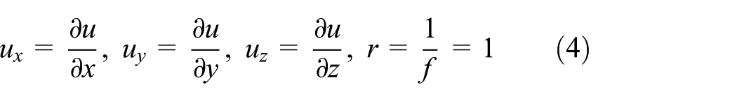
where f is the propagation speed of the distance field and is set to 1 in this work. Since the distance field in S(x, y, z) is 0, we apply the following boundary condition

$$u(x,y,z)=0\mathrm{in}S(x,y,z)$$

(2)

To simplify the notations, we rewrite equation (1) as follows

$$u_x^2+u_y^2+u_z^2=r^2$$

(3)

where

$$u_x=\frac{\partial u}{\partial x},u_y=\frac{\partial u}{\partial y},u_z=\frac{\partial u}{\partial z},r=\frac{1}{f}=1$$

(4)

Overview of the revised FMM

We compute the distance field using a revised fast marching method (RFMM). In this method, we divide all the voxels of the 3D image into three sets, DONE, CLOSE, and FAR, as shown in Figure 5. DONE contains those voxels, whose final distances have been computed. CLOSE keeps the voxels, which are immediately adjacent to the voxels of DONE. Other voxels are stored in FAR. Initially, the voxels of S(x, y, z) are inserted into DONE. Their distances are set to 0. Then the voxels adjacent to S(x, y, z) are searched, and their distances are computed using the distances of the voxels in DONE. These voxels are stored in CLOSE. The remaining voxels are moved to FAR and their distances are set to a number which is much larger than the extents of the BB in all the axes. In order to speed up the computation, CLOSE is implemented using a priority queue ²² such that the voxel belonging to CLOSE and having the smallest distance is always at the top position of CLOSE.

Figure 5.

Voxels of the 3D image are divided into three groups: DONE (light blue circles), CLOSE (red squares), and FAR (grid points).

The RFMM is carried out in an iterative manner. At each iteration, the top-most voxel of CLOSE is removed from CLOSE and is inserted into DONE. Then its neighbors, which are in CLOSE and FAR, are searched and the distances of these neighboring voxels are updated. After the updating, those neighbors, which are in FAR before the updating, are removed from FAR and are inserted into CLOSE. If a neighbor had already been in CLOSE before the updating, its position in CLOSE is adjusted according to its new distance value. The aforementioned computations are repeated until CLOSE becomes an empty set. Given an $N\times N\times N$ lattice, CLOSE will be empty after $O(N^3)$ iterations. In each iteration, $O(\log N)$ time steps are required for restructuring CLOSE. Thus, the time complexity of the revised FMM is bounded by $O(N^3\log N)$ .

The undetermined coefficient method for approximating derivatives

In the RFMM, the distance of each individual voxel is updated by solving equation (3). At first, we convert equation (3) into a quadratic polynomial. Then the two roots of the quadratic polynomial are calculated. Finally, the larger root is used to replace the distance of the voxel, if it is smaller than the old distance of the target voxel.

To convert equation (3) into a polynomial, we approximate the partial derivatives using an undetermined coefficient method. ²³ Assuming that the distance value of voxel V_i,j,k is denoted as u_i,j,k and the spatial gap between two adjacent voxels is 1, then the partial derivatives of the distance field at position (i, j, k) can be expressed as

$$\begin{array}{c}{u}_x=A{u}_{i-1,j,k}+B{u}_{i,j,k}+C{u}_{i+1,j,k}\hfill \\ u_y=D{u}_{i,j-1,k}+E{u}_{i,j,k}+F{u}_{i,j+1,k}\hfill \\ u_z=G{u}_{i,j,k-1}+H{u}_{i,j,k}+I{u}_{i,j,k+1}\hfill \end{array}$$

(5)

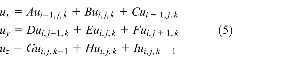
where A to I are coefficients to be determined. Initially they are 0. Then their values are calculated according to the following rules:

• If both V_i–1,j,k and V_i+1,j,k are in DONE: if u_i–1,j,k ≤ u_i+1,j,k, then A = –1, B = 1, and C = 0; else A = 0, B = –1, and C = 1.

• Else if only V_i–1,j,k is in DONE, A = –1, B = 1, and C = 0. Else if only V_i+1,j,k is in DONE, A = 0, B = –1, and C = 1.

• If both V_i,j–1,k and V_i,j+1,k are in DONE: if u_{i, j–1,k} ≤ u_{i j+1,k}, then D = –1, E = 1, and F = 0; else D = 0, E = –1, and F = 1.

• Else if only V_i,j–1,k is in DONE, D = –1, E = 1, and F = 0. Else if only V_i,j+1,k is in DONE, D = 0, E = –1, and F = 1.

• If both V_i,j,k–1 and V_i,j,k+1 are in DONE: if u_i,j,k–1 ≤ u_i,j,k+1, then G = –1, H = 1, and I = 0; else G = 0, H = –1, and I = 1.

• Else if only V_i,j,k–1 is in DONE, G = –1, H = 1, and I = 0. Else if only V_i,j,k+1 is in DONE, G = 0, H = –1, and I = 1.

The rationale of the undetermined coefficient method can be explained by Figure 6. This figure shows the rules for determining A, B, and C for calculating u_x at position (i, j, k): if both the neighbors of V_i,j,k in the x-axis are not in DONE, these two neighbors are ignored in the updating process, since their final distances have not been determined yet. Thus, A, B, and C are set to 0. If only one of the two neighbors is in DONE, this neighbor’s distance is used to estimate u_x. The x-derivative is approximated using either the forward or the backward difference method, depending on the position of this neighbor. If both neighbors are in DONE, we select the neighbor with smaller distance to estimate u_x. Hence, the resultant distance of V_i,j,k is minimized. The rules used to determine the coefficients for computing u_y and u_z can be explained by analogy.

Figure 6.

The coefficient determination method for computing u_x.

The updating method

Once these coefficients of equation (5) have been computed, we substitute equation (5) into equation (3) and form a quadratic polynomial

$$a{u}^2+\mathrm{bu}+c=0$$

(6)

where u is the distance value to be solved at position (i, j, k) and a, b, and c are the coefficients, which are defined as

$$\begin{array}{c}a=B^2+E^2+H^2\hfill \\ b=2[{\mathrm{ABu}}_{i-1,j,k}+{\mathrm{BCu}}_{i+1,j,k}+{\mathrm{DEu}}_{i,j-1,k}+{\mathrm{EFu}}_{i,j+1,k}\hfill \\ \multicolumn{1}{c}{+{\mathrm{GHu}}_{i,j,k-1}+{\mathrm{HIu}}_{i,j,k+1}]}\\ c=[A^2{u}_{i-1,j,k}^2+C^2{u}_{i+1,j,k}^2+D^2{u}_{i,j-1,k}^2+F^2{u}_{i,j+1,k}^2\hfill \\ \multicolumn{1}{c}{+G^2{u}_{i,j,k-1}^2+I^2{u}_{i,j,k+1}^2+2{\mathrm{ACu}}_{i-1,j,k}{u}_{i+1,j,k}}\\ \multicolumn{1}{c}{+2{\mathrm{DFu}}_{i,j-1,k}{u}_{i,j+1,k}+2{\mathrm{GIu}}_{i,j,k-1}{u}_{i,j,k+1}]-r_{i,j,k}^2}\end{array}$$

(7)

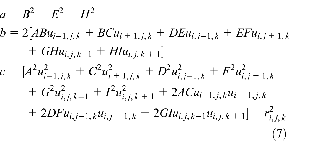
Since a is positive, the quadratic polynomial has a minimum extreme value at the position from which the distance field propagates to the current position (i, j, k).

Then the two roots of the quadratic polynomial of equation (6) are calculated. These roots are always real and positive. The root with larger magnitude is used as the new distance at position (i, j, k) if it is smaller than u_i,j,k. Intuitively, we should use the smaller root of the quadratic polynomial to update the distance value such that u_i,j,k would be minimized. However, in the RFMM, we select the larger root to update the distance. The verification and rationale of the RFMM are given in Appendix 1.

The Laplacian smoothing

It had been demonstrated by Sethian ¹⁷ that u(x, y, z) may be non-differentiable at some points, which are equidistant to multiple positions in S(x, y, z). This will create sharp corners and edges in the distance field. In this work, we apply a Laplacian filter upon the distance field to alleviate these geometrical features. The Laplacian filter is defined by Strikwerda ²⁴

$${\nabla }^{2}u=\frac{{\partial }^{2}u}{\partial x^2}+\frac{{\partial }^{2}u}{\partial y^2}+\frac{{\partial }^{2}u}{\partial z^2}=0$$

(8)

To prevent smoothing out the distance field, we set the following boundary conditions at S(x, y, z) and the boundaries of the BB

$$\begin{array}{c}u(x,y,z)=0,\forall (x,y,z)\in S(x,y,z)\hfill \\ u(x,y,z)=u^{*},\forall (x,y,z)\in \mathrm{\Gamma }\hfill \end{array}$$

(9)

where Γ and u* stand for the boundaries of the BB and the distance values of the points in the boundaries, respectively. Equation (8) is solved using the Gauss–Seidel method. The iteration is carried out in an alternating direction implicit (ADI) manner ²⁴ to speed up the convergence. In each iteration, two sweepings are performed, one from voxel (0, 0, 0) to voxel (N–1, N–1, N–1) and the other one in the opposite direction (assume that the lattice resolution is $N\times N\times N$ )

$$\begin{array}{c}{u}_{i,j,k}^{n+1/2}=\frac{1}{6}(u_{i-1,j,k}^{n+1/2}+u_{i,j-1,k}^{n+1/2}+u_{i-1,j,k-1}^{n+1/2}+u_{i+1,j,k}^n+u_{i,j+1,k}^n+u_{i,j,k+1}^n)\hfill \\ u_{i,j,k}^{n+1}=\frac{1}{6}(u_{i-1,j,k}^{n+1/2}+u_{i,j-1,k}^{n+1/2}+u_{i-1,j,k-1}^{n+1/2}+u_{i+1,j,k}^{n+1}+u_{i,j+1,k}^{n+1}+u_{i,j,k+1}^{n+1})\hfill \end{array}$$

(10)

In the proposed LM procedure, a layer of the distance field, which is close to S(x, y, z), will be extracted and treated as the final B-rep. Based on experiments, we found that a few iterations of the Laplacian smoothing are enough for creating a smooth B-rep (the creation method is presented in the following section). Thus, the ADI sweeping will be performed for no more than $O(\log N)$ times. An example is shown in Figure 7 to demonstrate the effects of the Laplacian smoothing. Figure 7(a) shows a layer of the distance field before the Laplacian smoothing. The same layer of the smoothed distance field is displayed in Figure 7(b). Based on these two images, we find that the roughness of the distance field is reduced after the Laplacian operation.

Figure 7.

A layer of distance field enclosing a carp model: (a) a layer of u(x, y, z) before the Laplacian smoothing and (b) the same layer after the Laplacian smoothing.

B-rep generation and printability

The distance field implicitly defines a level set. Each distance value is correspondent to a surface in the 3D space. Given u = 0, we can attain the preliminary iso-surface, since it is the boundary where the distance field originates. If S(x, y, z) forms a solid geometry after the morphological operations, this iso-surface can be used to define the outer surface of the target object. However, if S(x, y, z) is not closed even after the morphological operations, this new iso-surface is not closed either. It cannot serve as a geometrical representation in the LM procedure. Thus, under such situation, we will not retrieve an iso-surface using the iso-value u = 0.

On the contrary, a positive distance value u = t determines an iso-surface enclosing S(x, y, z). Unlike the preliminary iso-surface model, this new iso-surface model is always closed and defines a solid geometry. Its wall thickness is 2t. It is printable by 3D printers if its wall is thick enough (the wall should be wider than the diameter of the nozzle of the printer). Thus, at the final stage of the modeling process, we utilize the marching cube method to extract an iso-surface from the distance field and treat the resultant iso-surface as the B-rep of the target object.

Two types of B-rep could be created by the marching cube procedure, depending on S(x, y, z). If the S(x, y, z) is closed after the morphological operations, the B-rep contains two pieces of surfaces, one inside S(x, y, z) and the other outside S(x, y, z). Thus, the B-rep forms a hollow model with wall thickness equal to 2t. On the contrary, if S(x, y, z) is not closed, the B-rep contains only one offset surface which is solid and encloses S(x, y, z). A 2D example is shown in Figure 8 to illustrate these two cases. In Figure 8(a), the preliminary model S(x, y, z) is closed and the new iso-surface consists of two offset surfaces, one inside S(x, y, z) and the other outside S(x, y, z). The two offset surfaces define a hollow model whose wall thickness is twice the iso-value. The hollow model is represented by the shaded area and S(x, y, z) is depicted by the red dash line. In Figure 8(b), S(x, y, z) is not closed and the new iso-surface is comprised of an offset surface which completely surrounds S(x, y, z). The resultant model defines a solid object. The width of its interior part is twice the iso-value. In both cases, the new iso-surface forms a solid geometry, which is always printable by 3D printers.

Figure 8.

Two types of solid geometry generated by the LM procedure: (a) a hollow model defined by two offset surfaces and (b) a solid model defined by one offset surface.

Figure 9 demonstrates an example displaying the distance field and the B-rep. Figure 9(a) and (b) shows multiple and a single layer of the distance field surrounding the carp model, respectively. In Figure 9, the layer of the distance field defined by u = 0 is rendered in red, while other layers are shaded in white, yellow, green, and blue. The outer appearance of the final B-rep is shown in Figure 9(c). A cut-through image is presented in Figure 9(d) to show the internal structures of the B-rep model.

Figure 9.

(a) Multiple layers of the distance field; (b) a layer of the distance field; (c) outer appearance of the B-rep; and (d) wall thickness and internal structures of the B-rep.

Test results

The proposed geometrical modeling procedure had been implemented using C-language and OpenGL graphics libraries. The system architecture, computational flow, and variation of the geometry representation of the target model are displayed in Figure 10. Using this system, some tests had been conducted to verify the effectiveness of the proposed geometrical modeling procedure. The experimental environment, test data sets, and experimental results are presented in this section. Discussion and analysis of the experimental results will be given in the next section.

Figure 10.

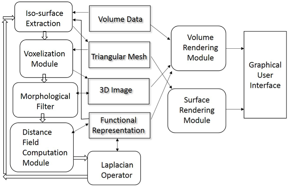
System architecture of the proposed LM procedure and the data flow.

Settings of the experiments and the data sets

This work focuses on the modeling process. The orientation, supporting structure construction, slicing, and G-code generation are performed using a free slicer, downloaded from the Internet. The physical models are printed using a fused deposition modeling (FDM) printer. The material of the filament is PLA (polylactide). The parameters of the FDM printer are shown in Table 1. The diameter of the nozzle is 0.4 mm. The layer thickness of the printed models is fixed at 0.1 mm, which is equal to the thinnest layer thickness printable by the 3D printer.

Table 1.

Settings of the 3D printer.

Parameters	Parameter values
LM modality	Fuse deposition modeling
Filament	PLA
Nozzle diameter	0.4 mm
Layer thickness	0.1 mm
Nozzle temperature	205°C

LM: layered manufacturing; PLA: polylactide.

Four test data sets are used in the experiments, including a CT head, a lobster, a carp, and a tooth model. These data sets are generated by CT-scans. Key information of these data sets is given in Table 2. The resolutions and intensity ranges are mentioned in the second and third columns, respectively. The iso-values of the target objects are depicted in the fourth column.

Table 2.

Test data sets.

Data sets	Resolutions	Intensity ranges	Iso-values
Lobster	301 × 324 × 56	0–255	35
CT head	256 × 256 × 113	0–3272	1500
Carp	256 × 256 × 256	0–255	50
Tooth	103 × 94 × 161	0–1300	500

CT: computerized tomography.

We generated the preliminary iso-surface models using the iso-surface extraction subroutine. The preliminary models are converted into 3D images and are filtered by the morphological operations. At the following stages, distance fields are computed in the 3D image spaces and smoothed by the Laplacian operator. Finally, the B-reps are created from the distance fields using the iso-surface extraction module. Table 3 contains some intrinsic information about the preliminary iso-surfaces, 3D images, and final B-reps. The numbers of triangles in the preliminary iso-surfaces are listed in the second column. The resolutions of the 3D images are revealed in the third column while the numbers of triangles in the final B-reps are shown in the fourth column. The dimension of each voxel of the 3D images is about $0.18\times 0.18\times 0.18\mathrm{mm}$ .

Table 3.

Metrics of the iso-surface models, 3D images, and B-reps.

Data sets	Numbers of triangles(preliminary iso-surfaces)	3D image resolutions	Numbers of triangles(final B-reps)
Lobster	324,364	422 × 120 × 411	792,728
CT head	601,966	259 × 377 × 347	3,865,472
Carp	206,040	431 × 176 × 94	703,000
Tooth	129,688	231 × 399 × 204	1,576,120

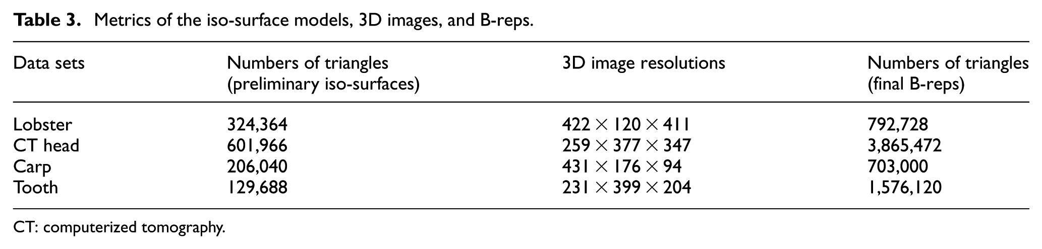
CT: computerized tomography.

Visualization of the modeling results and printed objects

Images of the preliminary iso-surfaces, 3D image models, and final B-reps are presented in Figures 2 and 11–13. Figure 2 illustrates the experimental results of the CT head data. Figure 2(a) of this figure shows the preliminary iso-surface (left), 3D image (middle), and final B-rep (right) of the skull. The B-rep model is superior to the preliminary iso-surface model in terms of surface quality and noise-level. Figure 2(b) displays the zoom-in images of the skull. The surfaces of the preliminary iso-surface and the B-rep are shown in the left and right images. The structures near the mouth and nose are better represented in the B-rep model. The holes and gaps are also filled. Based on these two images, the effectiveness of the proposed modeling procedure is verified.

Figure 11.

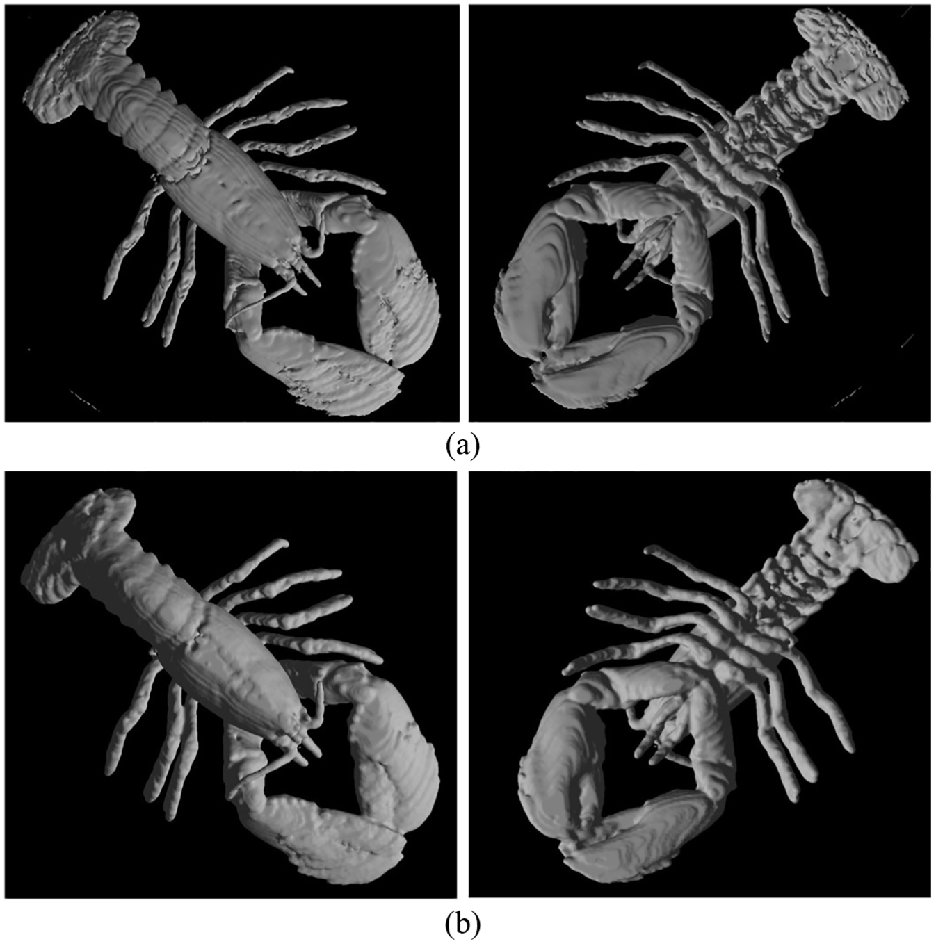
Experimental results using the lobster CT data: (a) the preliminary iso-surface model and (b) the B-rep model generated by the proposed modeling method.

Figure 12.

Experimental results of the carp data: (a) the preliminary iso-surface model, (b) the 3D image model, (c) the B-rep model, and (d) a cut-through image of the B-rep model to show the internal structures.

Figure 13.

Tests results of the tooth data set: (a) cut-through image of the preliminary iso-surface model, (b) 3D image model, and (c) a cut-through image of the final B-rep model.

Figure 11 displays four images of the preliminary iso-surface model and final B-rep of the lobster data set. Figure 11(a) contains the images of the preliminary iso-surface model. As shown in these images, the claws and legs contain small holes and gaps. The images of the final B-reps are displayed in Figure 11(b). These images show that the small holes and gaps are removed and the surface quality is greatly improved. The B-rep surface forms a solid geometry.

Test results using the carp model are displayed in Figure 12. The preliminary iso-surface is shown in Figure 12(a). The surface quality of this preliminary model is high. It contains almost no noise. However, this iso-surface defines a solid object. As the model is layered-manufactured, a lot of filament is wasted to fill the interior of the carp model. The other problem with the preliminary iso-surface model is that the internal structures will be filled by the 3D printer, since the whole model is regarded as a single solid object by the slicer. The B-rep model produced by the proposed LM procedure is illustrated in Figure 12(c). A cut-through image of the B-rep model is given in Figure 12(d). As this image shows, the resultant B-rep defines a hollow object and preserves the internal structures of the carp model. Hence, the 3D printer will not fill the interior space of the B-rep. This functionality cannot be accomplished using conventional iso-surface modeling methods.

The tooth model produces similar results. Some test results of this data set are shown in Figure 13. The preliminary iso-surface is shown in Figure 13(a), while the final B-rep of the tooth is displayed in Figure 13(c). Both models are cut to reveal the internal structures. The preliminary iso-surface represents a solid object. When being printed, the space between the tooth surface and the internal structures will be filled. However, in the B-rep model, the outer surface as well as the internal structures of the tooth are modeled as hollow objects. The gap between them will be preserved as the model is physically printed.

Some photos of the printed physical models are shown in Figure 14. These physical models are not polished. The surface qualities of these physical models are influenced by the precision of the 3D printer and the filament. The skull structure of the CT head data is very complicated. The slicer created a lot of supporting structures beneath and inside the model. As the supporting structures were removed, the physical model suffered from rough surfaces and broken parts. The same phenomenon occurs in the physical model of the lobster data. However, these physical models prove that the resultant B-reps generated by our modeling system are printable even using a low-end 3D printer. The printed models convey the key geometrical features of the target objects. They are useful tools for studying the shapes and structures of the hidden objects of the volume data sets.

Figure 14.

The printed models, upper left: the CT head model, upper right: the carp model, lower left: the tooth model, and lower right: the lobster model.

Discussion and analysis

In the proposed modeling procedure, the preliminary iso-surface model of the target object is discretized into a 3D image using a lattice prior to the morphological operations and the distance field computation. In this section, the effects of the lattice resolution on the quality of the final B-rep and the computational costs are presented and analyzed. The proposed modeling procedure requires users’ interferences to achieve better results. The issues about human interaction are also discussed in this section.

Model precision and computational costs

To uncover the influence of lattice resolution on the surface quality of the final B-rep, a test is conducted using three lattices of different resolutions to create B-reps for the CT head. Some information acquired from the test are presented in Table 4. The lattice resolutions are listed in the first column. The numbers of triangles of the resultant B-reps are depicted in the second column while the voxel sizes of the lattices are presented in the third column.

Table 4.

B-rep models of different resolutions.

Resolutions ofthe lattices	Numbers of trianglesin the B-reps	Voxel width (mm)
59 × 84 × 80	99,596	0.8
114 × 162 × 156	545,380	0.4
223 × 318 × 307	2,835,716	0.2

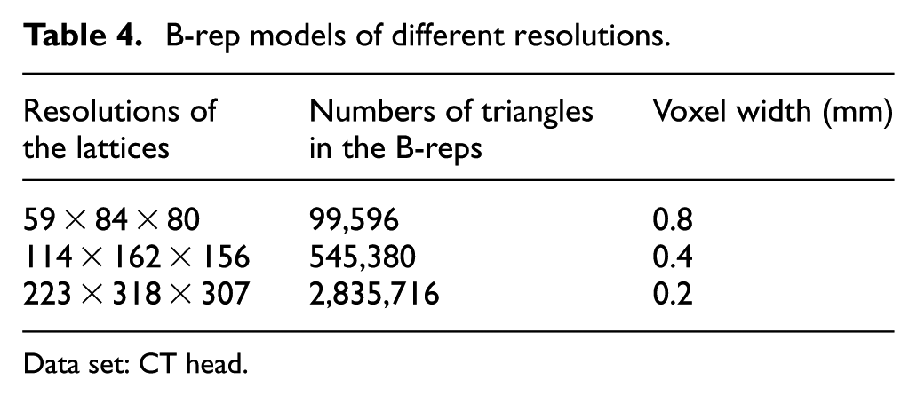
Data set: CT head.

Figure 15 demonstrates the 3D images and final B-reps of the skull, generated using these three lattices. The upper part of the figure shows the 3D image models while the lower part of the figure displays the final B-reps. The results show that the B-rep generated using the finest lattice is superior to those produced using the coarser lattices. Thus, using a high-resolution lattice in the modeling process will result in a better B-rep. Photos of the printed objects are shown in Figure 16. Comparing these three pictures, we found that the surface qualities of the printed models are also affected by the lattice resolution. Fine lattices produce better physical models.

Figure 15.

Three-dimensional image and B-rep models generated using low-, middle-, and high-resolution lattices: (a) voxel-based models of low, middle, and high resolutions and (b) B-rep models of low, middle, and high resolution.

Figure 16.

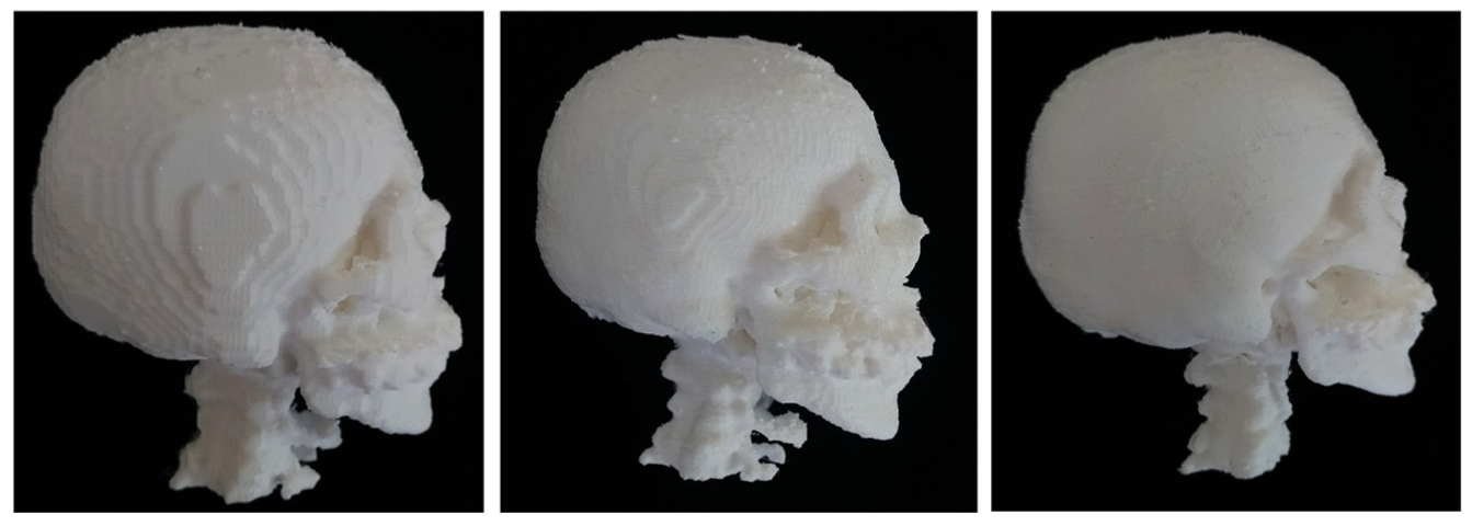
Printed models of the CT head using three levels of lattices, left: low resolution, middle: middle resolution, and right: high resolution.

The effect of the lattice resolution upon the qualities of the B-reps and printed models can be explained as follows: by using a finer lattice, more details of the target model can be represented as shown in Table 4. Thus, the geometrical precision is improved. When computing the distance field, we used the undetermined coefficient method to approximate the partial derivatives. Thus, truncation errors are inevitable in the computation. As the lattice resolution increases, these truncation errors decrease and the numerical accuracy is enhanced. Combining these factors, the qualities of the B-rep and printed model will be improved as the lattice resolution is raised.

However, using fine lattices in the modeling process comes with prices. The memory usage of the lattice grows cubically as the resolution increases. The available memory space lays a limitation for the lattice resolution. The other concern is the diameter of the nozzle of the 3D printer. As the lattice resolution gradually increases, the sizes of the triangles of the B-rep decrease. If the triangles of the B-rep are smaller than the nozzle’s diameter, we will not gain much improvement on the printed object. The other problem is the computational costs. The time complexity of the geometrical modeling procedure is dominated by the distance field computation and the Laplacian filtering process. Given an $N\times N\times N$ lattice, the time complexity is bounded by $O(N^3\log N)$ . As the lattice resolution grows, the time complexity increases too.

Users’ interferences

The achievement of the work presented by Giannopoulos et al. ⁷ is significant. However, the modeling tasks in their work require a lot of human efforts and expertise. In the proposed LM procedure, only the calculation of iso-value and the morphological operations need users’ involvement. Other stages require very limited input from the users. To determine a good iso-value for creating the preliminary iso-surface model, the users have to tune the transfer function and to volume-render the data set interactively, as shown in Figure 3. Since the rendering computation is sped-up by the graphics processing unit (GPU), computational speed is not a concern. However, background knowledge about the data set is helpful in finding the optimal iso-value.

The proposed LM procedure performs a closing operation upon the 3D image to fill small gaps and holes. Nonetheless, it is well known that the closing operation may merge two separate parts into one. ²¹ An example is presented in Figure 17. In this case, the closing operator is accomplished by applying three dilations and three erosions. The dilation computations merge two legs of the lobster, though they successfully fill the holes in the legs. In this work, the closing operation is semi-automatically carried out. The numbers and orders of the dilations and erosions are determined by the users. The users may need to tune the process, if the results do not meet the expectation.

Figure 17.

The closing operator may merge separate parts, if these parts are close: (a) legs of preliminary iso-surface model and (b) legs of B-rep model.

Conclusion

In this article, we present a modeling procedure to construct B-reps of scanned objects from CT-scan and MRI data sets. The resultant B-reps will be input models of LM for various medical applications. In the proposed procedure, the target models are represented by iso-surfaces, 3D images, and distance fields at different stages of the modeling process. Therefore, we can utilize morphological and Laplacian operators to improve the target models. The proposed modeling procedure is capable of generating not only solid models but also hollow ones with varying wall thickness. The B-reps, produced by the proposed procedure, form watertight solid geometries. They are always printable by 3D printers. Compared with previous work, for example, the works performed by Giannopoulos et al., ⁷ our modeling procedure requires less human interference. However, users’ input is required if we want to achieve better B-reps. In this work, we also propose a revised FMM for computing distance fields. Compared with the algorithms of Sethian ¹⁷ and Zhao, ¹⁸ our method is more elegant and easier to implement.

Several experiments have been conducted using the proposed modeling method. The test results show that the proposed modeling procedure successfully builds B-reps for various CT-scan data sets. By further analyzing the test results, we found that the surface quality and precision of the B-reps and printed objects are influenced by the resolution of the underlying lattices used in the voxelization step.