Spreadsheet-based method for predicting temperature dependence of fracture toughness in ductile-to-brittle temperature region

Abstract

A spreadsheet-based simplified and direct toughness scaling method to predict the temperature dependence of fracture toughness J_c in the ductile-to-brittle transition temperature region is proposed. This method uses fracture toughness test data and the Ramberg–Osgood exponent and yield stress at the reference temperature, and yield stress at the temperature in interest to predict J_c. The physical basis of the simplified and direct toughness scaling method is the strong correlation between J_c and yield stress. The simplified and direct toughness scaling method was validated for Cr–Mo steel Japan Industrial Standard SCM440 and 0.55% carbon steel Japan Industrial Standard S55C by comparing the simplified and direct toughness scaling prediction results with the median results of an experiment performed at four temperatures ranging from −55°C to 100°C and at three temperatures ranging from −85°C to 20°C, respectively. The simplified and direct toughness scaling method can predict J_c from both low to high temperatures, and vice versa. Thus, 12 and 6 predictions were made for each material. The prediction discrepancy for these 18 cases ranged from −50.4% to +25.8% and the average absolute discrepancy was 22.1%. These results were acceptable considering the large scatter generally observed with J_c. In particular, in case of predicting J_c at temperatures higher than the lowest temperature of −55°C for SCM440, the simplified and direct toughness scaling method predicted J_c more realistically than the American Society for Testing and Materials E1921 master curve approach. Although the simplified and direct toughness scaling method requires additional tensile test data compared with the master curve approach, the acceptable prediction accuracy at high temperatures seems beneficial because the mass and time required for tensile tests are admissible.

Introduction

To evaluate the structural integrity of deteriorated steel and cracked structures over time in the ductile-to-brittle transition temperature (DBTT) region, it is necessary to understand the following three characteristics of the fracture toughness J_c of the member, that is, (1) large temperature dependence (approximately 1000% change with a temperature change of 100°C),^1–3 (2) J_c–specimen size dependence,^4–11 and (3) large scatter,^12,13 as shown in Figure 1. The temperature dependence on J_c has been attributed to embrittlement caused by a decrease in temperature. ² Owing to its simplicity, the empirical American Society for Testing and Materials (ASTM) E1921 master curve (MC) approach^2,14,15 has attracted increasing attention, although some studies have noted that the prediction needs to be improved for relatively high temperatures. ¹ In contrast, the authors’ group has been developing an analytical approach that uses three-dimensional elastic–plastic finite element analysis (3D EP-FEA) with a focus on transferring the mean J_c between different specimen sizes^9–11 and temperatures. ¹⁶ The theoretical basis of this analytical approach is the perspective that the scaled fracture stress is independent of the test specimen size and temperature.

Figure 1.

Temperature dependence of fracture toughness J_c.

Assuming that the fracture in the DBTT region occurs under the small-scale yielding (SSY) condition and Ramberg–Osgood (R–O) stress–strain relationship, the author’s group proposed the stress distribution T-scaling method to scale the EP-FEA crack opening stress distribution at fracture at different temperatures. ¹⁶ Accordingly, by assuming the fracture stress for slip-induced cleavage fracture is temperature independent, ¹⁷ the authors applied the T-scaling method to scale the critical distance at different temperatures and enabled the direct prediction of the ratio of fracture load P_c between two temperatures (referred to as the critical distance scaling (CDS) method, which is briefly introduced in section “CDS method”). ¹⁶ The CDS method indicated a strong dependence of P_c on (1/σ₀) (σ₀: R–O fitting parameter correlated with the yield stress). Finally, Ishihara et al. ¹⁶ proposed a framework for predicting J_c at a temperature of interest T_i from J_c at a reference temperature T_r (see Figure 2). The framework was validated at temperatures ranging from −25°C to +20°C for Japan Industrial Standard (JIS) S55C and −100°C to −64°C for the A533B reactor pressure vessel steel.

Figure 2.

Three-step procedure to predict the J_c temperature dependence using the CDS method. ¹⁶ Details of these procedures are explained in section “CDS method.” This study proposes a simplified method that does not require performing EP-FEA.

This framework is advantageous compared with the MC approach because (1) fracture toughness tests can be performed at arbitrarily selected single temperatures (cf. the MC approach recommends preliminary tests to be performed so that the test temperature is close to the estimated reference temperature T₀), and (2) J_c at T_i can be predicted by performing EP-FEA.

The disadvantage of the proposed framework compared with the MC approach is that it requires tensile test results at T_r and T_i, specifically, the stress–strain relationships at these temperatures to obtain R–O parameters α and n and to run EP-FEA at T_i. However, this disadvantage seems to be allowable because the tensile test specimens are small compared with the fracture toughness test specimens and they show small scatter; therefore, two tests are usually enough.

Another disadvantage is that detailed 3D EP-FEA is required for J_c temperature dependence prediction. Practitioners and design engineers suggested that because they were unfamiliar with 3D EP-FEA, its use in the framework for predicting the J_c temperature dependence was a bottleneck.

Thus, in this study, the J_c temperature dependence framework shown in Figure 2 ¹⁶ is extended so that J_c at a temperature of interest T_i can be predicted using spreadsheet calculations with minimal test data (specifically, fracture toughness test results J_c and P_c at a single arbitrary temperature T_r, R–O exponent n at T_r, and σ_YS at both T_r and T_i). For this purpose, (1) the P_c ∝ 1/σ_YS relationship was discussed and validated in a wide temperature range (target temperature range is over 100°C) for more than one material, and (2) a simplified method that uses the P_c ∝ 1/σ_YS relationship to predict the J_c temperature dependence using spreadsheet calculations was proposed and validated. This method was referred to as the Simplified and Direct Toughness Scaling (SDTS) method.

The P_c ∝ 1/σ_YS relationship and the SDTS method was validated for Cr–Mo steel JIS SCM440% and 0.55% carbon steel JIS S55C for a temperature range of −55°C to 100°C and −85°C to 20°C, respectively. The prediction discrepancy for these 18 cases ranged from −50.4% to +25.8%, and average absolute discrepancy was 22.1%. These results were acceptable considering the large scatter generally observed with J_c. In particular, in case of predicting J_c at temperatures higher than the lowest temperature of −55°C for SCM440, the SDTS method predicted J_c more realistically than the MC approach. Although the SDTS method requires additional tensile test data compared with the MC approach, the prediction improvement at high temperatures seems beneficial because the mass and time required for tensile tests are admissible.

CDS method

First, the CDS method to predict the ratio of fracture load P_c between two temperatures and a framework for J_c temperature dependence prediction (Figure 2) is briefly introduced. ¹⁶ Assuming that (1) the stress–strain relationship for a material is described by the R–O power law as

$$\frac{\epsilon }{{\epsilon }_0}=\frac{\sigma }{{\sigma }_0}+\alpha {\left(\frac{\sigma }{{\sigma }_0}\right)}^n$$

(1)

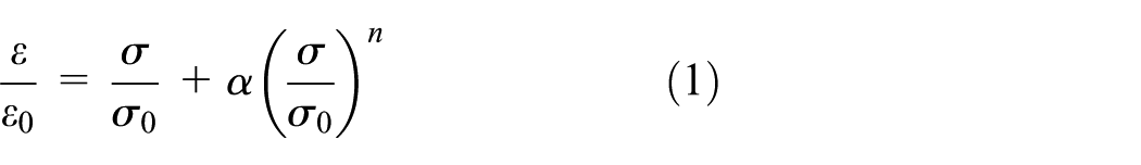
where σ₀ and ε₀ is the reference stress and strain, respectively; (2) fracture occurs in the DBTT region under the SSY condition, where the EP-FEA stress distribution is enveloped by the theoretical stress intensity factor (SIF) K and Hutchinson–Rice–Rosengren (HRR) stress distributions; ¹⁷ (3) the fracture stress for a slip-induced cleavage fracture is temperature independent; ¹⁸ and (4) the J-integral J_e under SSY is equal to (K_e) ² /E′, where K_e is the elastic SIF and E′ = E/(1 − ν²) (E: Young’s modulus, ν: Poisson’s ratio); the relationship between the two fracture SIFs K_cr and K_ci at the reference temperature T_r and temperature of interest T_i, respectively, was deduced as shown below. Because fracture load P_c is proportional to K_c, the fracture load (P_ci) can be predicted directly from the fracture load at T_r (P_cr), and this is called the CDS method

$$\begin{array}{c}{T}_1<T_{\mathrm{r}}\hfill \\ \frac{P_{\mathrm{c}1}}{P_{\mathrm{cr}}}=\frac{K_{\mathrm{c}1}}{K_{\mathrm{cr}}}=\left(\frac{{\sigma }_{0\mathrm{r}}}{{\sigma }_{01}}\right)\frac{{\left(2\pi \right)}^{\frac{n_{\mathrm{r}}+1}{2(n_{\mathrm{r}}-1)}}}{{\left(2\pi \right)}^{\frac{n_1+1}{2(n_1-1)}}}\frac{{\left(\frac{I_{n1}{\alpha }_1}{(1-{\nu }^2)}\right)}^{\frac{1}{n_1-1}}}{{\left(\frac{I_{n\mathrm{r}}{\alpha }_{\mathrm{r}}}{(1-{\nu }^2)}\right)}^{\frac{1}{n_{\mathrm{r}}-1}}}\frac{{\tilde{\sigma }}_{22}{(n_{\mathrm{r}},0)}^{\frac{n_{\mathrm{r}}+1}{n_{\mathrm{r}}-1}}}{{\tilde{\sigma }}_{22}{(n_1,0)}^{\frac{n_1+1}{n_1-1}}},\hfill \\ T_{\mathrm{r}}<T_2\hfill \\ \frac{P_{\mathrm{c}2}}{P_{\mathrm{cr}}}=\frac{K_{\mathrm{c}2}}{K_{\mathrm{cr}}}={\left(\frac{{\sigma }_{0\mathrm{r}}}{{\sigma }_{02}}\right)}^{\frac{n_2+1}{2}}\frac{{\left(2\pi {\left\{{\tilde{\sigma }}_{22}(n_{\mathrm{r}},0)\right\}}^2\frac{(1-{\nu }^2)}{I_{n\mathrm{r}}{\alpha }_{\mathrm{r}}}\right)}^{\frac{n_2+1}{2(n_{\mathrm{r}}-1)}}}{{\left(2\pi {\left\{{\tilde{\sigma }}_{22}(n_2,0)\right\}}^2\frac{(1-{\nu }^2)}{I_{n2}{\alpha }_2}\right)}^{\frac{n_2+1}{2(n_2-1)}}}\hfill \\ \multicolumn{1}{c}{{\left(\frac{{\tilde{\sigma }}_{22}(n_{\mathrm{r}},0)}{{\tilde{\sigma }}_{22}(n_2,0)}\right)}^{\frac{n_2+1}{2}}}\end{array}$$

(2)

where I_n and ${\tilde{\sigma }}_{22}(n,0)$ are parameters used in HRR stress distribution definition that depend on n. ¹⁹ Suffixes for these parameters indicate the corresponding temperature.

The CDS method was validated experimentally in the temperature range of −25°C to +20°C for 0.55% carbon steel JIS S55C (σ₀: 444–394 MPa, α: 2.08–1.85, and n: 4.63–4.71), and −100°C to −64°C for the A533B reactor pressure vessel steel (σ₀: 640–544 MPa, α: 4.18–3.77, and n: 6.05–5.85). In addition, the CDS method proved to be applicable for K_Jc/K_c ≤ 1.9; although this is not expected from the classical definition of the SSY condition, it was found to satisfy the redefined SSY condition in which the EP-FEA stress distribution is enveloped by the theoretical K and HRR stress distributions. Here, K_Jc is the fracture toughness J_c converted to SIF, and K_c is the SIF corresponding to the fracture load P_c of the specimen. ¹⁶

Based on equation (2), the following three-step framework was proposed to predict the J_c at temperature in interest T_i from minimal experimental data obtained at reference temperatures T_r and T_i (Figure 2): ¹⁶

1. Obtain the mean fracture load P_crave at reference temperature T_r and perform tensile tests at both T_r and T_i to obtain stress–strain relationships and R–O parameters;

2. Predict the fracture load P_ci at T_i using equation (2);

3. Finally, perform EP-FEA at T_i up to the predicted fracture load P_ci and predict the fracture toughness as J corresponding to P_ci.

Interestingly, the results for the aforementioned two materials showed the following approximate relationship

$$\frac{P_{\mathrm{ci}}}{P_{\mathrm{cr}}}\approx \frac{{\sigma }_{0\mathrm{r}}}{{\sigma }_{0\mathrm{i}}}\approx \frac{{\sigma }_{\mathrm{YSr}}}{{\sigma }_{\mathrm{YSi}}}$$

(3)

irrespective of whether T₁ < T_r or T_r < T₂, though equation (2) gives different expressions for these two cases.

Equation (3) is understood as showing P_c’s strong yield stress dependence; this does not contradict with equation (2) on the point that the R–O parameter n shows small temperature dependence and that α tends to decrease with temperature. ²⁰ Specifically, by substituting n₁ = n₂ = n

$$\begin{array}{c}{T}_1<T_{\mathrm{r}}\hfill \\ \frac{P_{\mathrm{c}1}}{P_{\mathrm{cr}}}=\frac{K_{\mathrm{c}1}}{K_{\mathrm{cr}}}=\left(\frac{{\sigma }_{0\mathrm{r}}}{{\sigma }_{01}}\right){\left(\frac{{\alpha }_1}{{\alpha }_{\mathrm{r}}}\right)}^{\frac{1}{n-1}}\hfill \\ T_{\mathrm{r}}<T_2\hfill \\ \frac{P_{\mathrm{c}2}}{P_{\mathrm{cr}}}=\frac{K_{\mathrm{c}2}}{K_{\mathrm{cr}}}={\left(\frac{{\sigma }_{0\mathrm{r}}}{{\sigma }_{02}}\right)}^{\frac{n+1}{2}}{\left(\frac{{\alpha }_2}{{\alpha }_{\mathrm{r}}}\right)}^{\frac{n+1}{2(n-1)}}\hfill \end{array}$$

(4)

is deduced. For T₁ < T_r, the relationship P_c ∝ 1/σ_YS is directly deduced. For T_r < T₂, the relationship P_c ∝ 1/σ_YS is numerically possible because σ₀ and α show inverse tendency with temperature.

Equation (3) was considered useful because in many cases, although tensile tests are performed as check tests and σ_YS is available, the detailed stress–strain relationship is not determined in many cases and thus R–O parameters, which are necessary to predict P_ci by equation (2), are not available. This semi-analytical empirical P_c prediction method shown in equation (3) was called the simplified and direct scaling (SDS) method.

Thus, the SDS method was validated in a wide temperature range (target temperature range is over 100°C) for more than one material. Then, a simplified spreadsheet-based method was proposed to predict the J_c temperature dependence using the SDS method, so that the time-consuming EP-FEA is not necessary. Finally, the proposed method was validated by comparing the predicted results with the experimental results.

Material

Materials

The materials considered are 0.55% carbon steel JIS S55C and Cr–Mo steel JIS SCM440, whose room temperature falls within the DBTT region. The S55C plate was quenched at 850°C and tempered at 550°C, and the SCM440 plate was used as received. Tables 1 and 2 show the chemical compositions of S55C and SCM440, respectively, and they indicate that the specimen materials met the JIS G 4051 and JIS G 4053 standards.

Table 1.

Chemical compositions of test specimens in wt% for S55C.

JIS S55C	C	Si	Mn	P	S	Cu	Ni	Cr
Specified	0.52–0.58	0.15–0.35	0.60–0.90	≤0.030	≤0.035	≤0.30	≤0.20	≤0.15
Check analysis	0.54	0.17	0.61	0.014	0.003	0.10	0.06	0.12

JIS: Japan Industrial Standard.

Table 2.

Chemical compositions of test specimens in wt% for SCM440.

JIS SCM440	C	Si	Mn	P	S	Cu	Ni	Cr	Mo
Specified	0.38–0.43	0.15–0.35	0.60–0.90	≤0.030	≤0.035	≤0.30	≤0.20	0.90–1.20	0.15–0.30
Check analysis	0.39	0.17	0.62	0.011	0.002	0.10	0.07	1.02	0.17

JIS: Japan Industrial Standard.

Charpy impact tests

Charpy impact tests were conducted for the two materials in accordance with JIS Z 2242 ²¹ using 2-mm-deep 45° V-notched specimens with dimensions of 10 mm × 10 mm × 55 mm. The results are shown in Figure 3. For S55C, −166°C and −85°C were selected for the lower shelf region and −45°C and 20°C were selected for the DBTT region. For SCM440, −166°C and −110°C were selected for the lower shelf region and −55°C, 20°C, 60°C, and 100°C were selected for the DBTT region. Because the DBTT differs for the Charpy and fracture toughness tests, tensile and fracture toughness tests were performed at all of these temperatures (indicated in red in Figure 3).

Figure 3.

Charpy impact test results for (a) S55C and (b) SCM440.

Tensile tests

Next, stress–strain relationships were obtained for the selected temperatures in accordance with JIS Z 2241. ²² JIS standard 6-mm-diameter round bar specimens with 30-mm gage length were used. Up to 0.2% proof stress, the load rate was set at 20 MPa/s. Beyond 0.2% proof stress, the load rate was set at 30%/min, and this met the requirement of the standard 3–30 MPa/s up to 0.2% proof stress and 18%–48%/min beyond 0.2% proof stress.

Tables 3 and 4 show tensile test results together with R–O parameters for S55C and SCM440, respectively. The results obtained in the DBTT region, decided from the following fracture toughness tests, are listed. σ_B, σ_YS, and σ_0.2 are the tensile strength, yield stress, and 0.2% proof stress, respectively. SCM440 does not show a clear yield point, and thus, σ_YS was not listed. Linear least squares regression analyses were performed on the logarithms of σ/σ₀ and plastic component ε_p/ε₀ to obtain α and n in equation (1); this is similar to the procedure used by James ²⁰ for ASTM 302-B steel. R² is the coefficient of determination for the fitted curve compared with each test result. S55C shows a clear yield point, and σ₀ was set as σ_YS and ε₀ was set as σ_YS/(Young’s modulus). SCM440 does not show a clear yield point, and σ₀ was set as 0.2% proof stress and ε₀ was fixed as 0.002. The lowest mean R² was 0.9971 for S55C at −45°C. The R–O parameters for two specimens were averaged and used for data analysis in the following section.

Table 3.

Tensile test results (σ_B, σ_YS, and σ_0.2 are the tensile strength, yield stress, and 0.2% proof stress, respectively) and R–O parameters (σ₀, α, and n) for S55C in the DBTT region.

T (°C)		σ B (MPa)	σ YS (MPa)	σ 0.2 (MPa)	Elongation (%)	σ 0 (MPa)	α	n	R 2
20	1	684.0	399.0	378.0	20.0	399.0	1.770	5.160	0.9981
	2	686.0	408.0	385.0	22.0	408.0	1.882	5.211	0.9979
	Mean	685.0	403.5	381.5	21.0	403.5	1.83	5.19
−45	1	778.0	487.0	469.0	23.0	487.0	1.829	5.411	0.9991
	2	776.0	483.0	480.0	22.0	483.0	2.342	5.006	0.9971
	Mean	777.0	485.0	474.5	22.5	485.0	2.09	5.21
−85	1	821.0	584.0	560.0	24.0	584.0	3.923	4.985	0.9988
	2	827.0	578.0	563.0	24.0	578.0	3.871	4.731	0.9991
	Mean	824.0	581.0	561.5	24.0	581.0	3.90	4.86

DBTT: ductile-to-brittle transition temperature; R–O: Ramberg–Osgood.

R ² is the coefficient of determination for the fitted curve compared with each test result.

Table 4.

Tensile test results (σ_B and σ_0.2 are the tensile strength and 0.2% proof stress, respectively) and R–O parameters (σ₀, α, and n) for SCM440 in the DBTT region.

T (°C)		σ B (MPa)	σ YS (MPa)	σ 0.2 (MPa)	Elongation (%)	σ 0 (MPa)	α	n	R 2
100	1	696.0		406.0	14.5	406.0	1.460	5.128	0.9991
	2	712.0		414.0	14.5	414.0	1.423	5.153	0.9996
	Mean	704.0		410.0	14.5	410.0	1.44	5.14
60	1	764.0		450.0	16.5	450.0	1.545	5.015	0.9997
	2	724.0		419.0	16.5	419.0	1.470	5.058	0.9981
	Mean	744.0		434.5	16.5	434.5	1.51	5.04
20	1	794.0		456.0	17.0	456.0	1.620	4.732	0.9988
	2	798.0		461.0	17.0	461.0	1.632	4.800	0.9989
	Mean	796.0		458.5	17.0	458.5	1.63	4.77
−55	1	857.0		509.0	14.0	509.0	1.907	4.836	0.9992
	2	891.0		538.0	17.0	538.0	2.007	4.904	0.9992
	Mean	874.0		523.5	15.5	523.5	1.96	4.87

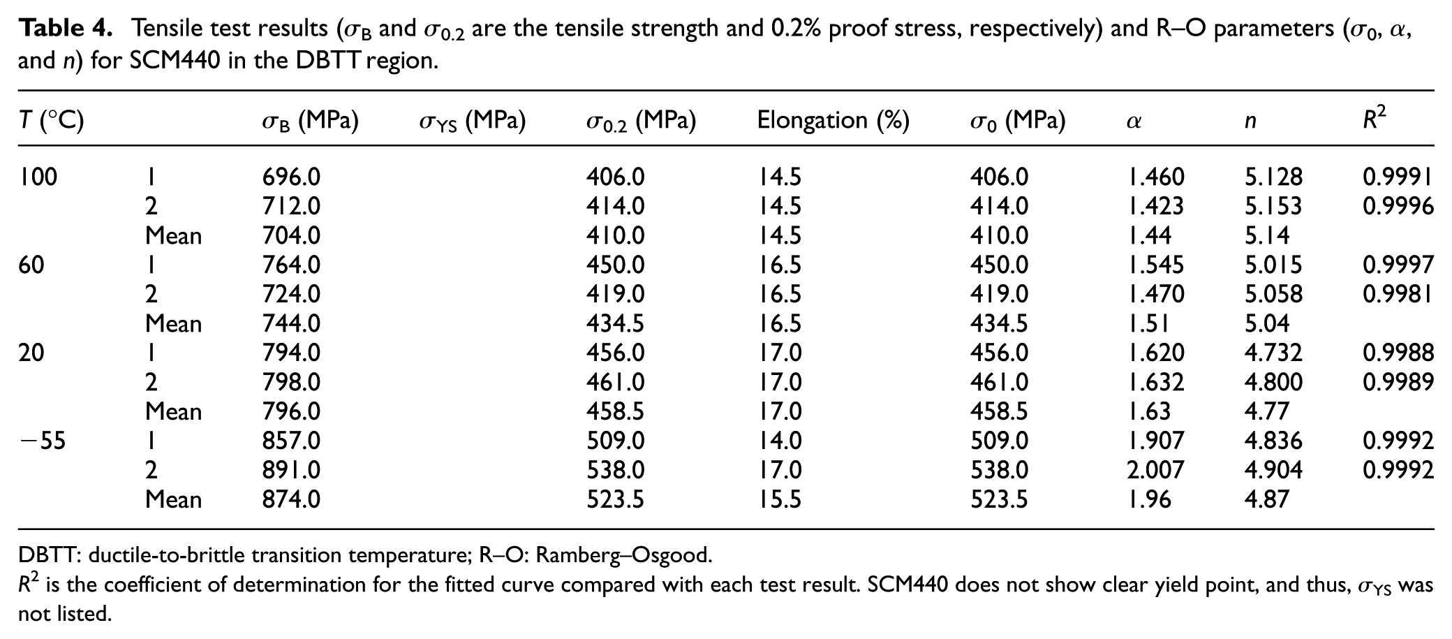
DBTT: ductile-to-brittle transition temperature; R–O: Ramberg–Osgood.

R ² is the coefficient of determination for the fitted curve compared with each test result. SCM440 does not show clear yield point, and thus, σ_YS was not listed.

Figure 4 shows the temperature dependence of the nominal yield stress σ_YS, tensile stress σ_B, and R–O parameter σ₀. Note that σ_YS for SCM440 is the 0.2% proof stress. Figure 5 shows the temperature dependence of the other R–O parameters n and α.

Figure 4.

Relationship between tensile properties and tested temperature T for (a) S55C and (b) SCM440. σ₀ is the R–O parameter related to σ_YS.

Figure 5.

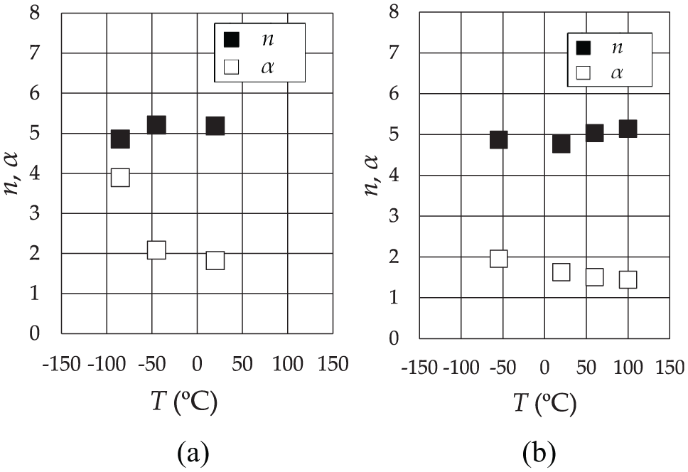
Relationship between R–O parameters and tested temperature T for (a) S55C and (b) SCM440.

According to Figure 5, the R–O parameters n and α are only slightly dependent on temperature in the DBTT region. The n for S55C at −85°C in the lower-shelf region showed values close to those in the DBTT region. However, α showed a significant change. As a small temperature dependence of n and α is a prerequisite for applying the SDS method, the method’s validation was examined using the DBTT temperature data along with the data at −85°C for S55C.

Fracture toughness test

Fracture toughness test procedure

Fracture toughness tests were conducted in accordance with ASTM E1921² using single-edge notched bend bar (SE(B)) test specimens of width W = 25 mm, thickness-to-width ratio of B/W = 0.5, and support span S = 4W, as shown in Figure 6. The specimens were sampled in the T–L direction in accordance with ASTM E399. ²³

Figure 6.

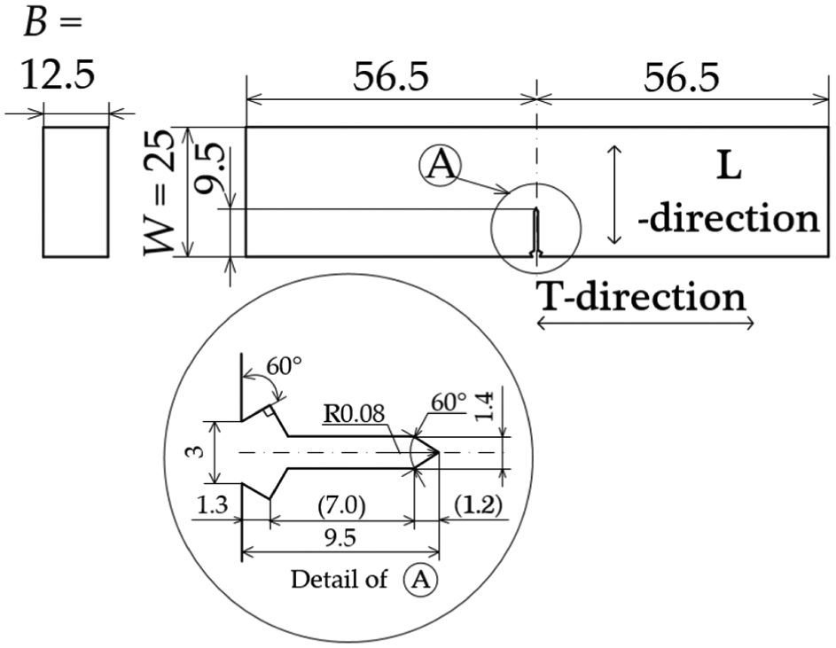
Dimensions of SE(B) fracture toughness test specimen. All dimensions are in millimeters. The support span was 4W, with width W = 25 mm.

Fatigue precracks of 3 mm were introduced at room temperature from the machined notch tip such that the initial crack length a prior to fracture testing was in the range of a/W = 0.496–0.504 (standard requirement: a/W = 0.45–0.55). These precracks were inserted with loads corresponding to K_max = 20.8 and 14.0 MPam^1/2 at the initial and final stages, respectively (standard requirement at the initial stage is K_max ≤ 25 MPam^1/2 and at the final stage is K_max ≤ 15 MPam^1/2). The maximum reduction in P_max in these steps was 15.3%; this satisfies the requirement of reduction of ≤20%. The load ratio R = P_min/P_max was 0.1, and the load frequency was 10 Hz. The fatigue precrack propagation was measured automatically using a clip gauge by applying the compliance method.

In fracture toughness tests, the loading rate was set to 1.2 MPam^1/2/s (standard requirement: 0.1–2.0 MPam^1/2/s). The specimen temperature was maintained at T ± 1°C for 30 min (standard requirement: T ± 3°C for 15 min).

Tables 5 and 6 show the test results, where μ and ∑ are the median and standard deviation of each quantity, respectively. P_c is the fracture load, and K_c is the SIF K calculated using the crack depth a at P_c with the SIF equation for SE(B) according to ASTM E1921² as follows

$$\begin{array}{c}\multicolumn{1}{c}{K=\left[\frac{\mathrm{PS}}{{\left(B{B}_{\mathrm{N}}\right)}^{\frac{1}{2}}{W}^{\frac{3}{2}}}\right]}\\ \multicolumn{1}{c}{\frac{3{\left(\frac{a}{W}\right)}^{\frac{1}{2}}\{1.99-\left(\frac{a}{W}\right)(1-\frac{a}{W})[2.15-3.93\left(\frac{a}{W}\right)+2.7{\left(\frac{a}{W}\right)}^2]\}}{2[1+2\left(\frac{a}{W}\right)]{(1-\frac{a}{W})}^{\frac{3}{2}}}}\end{array}$$

(5)

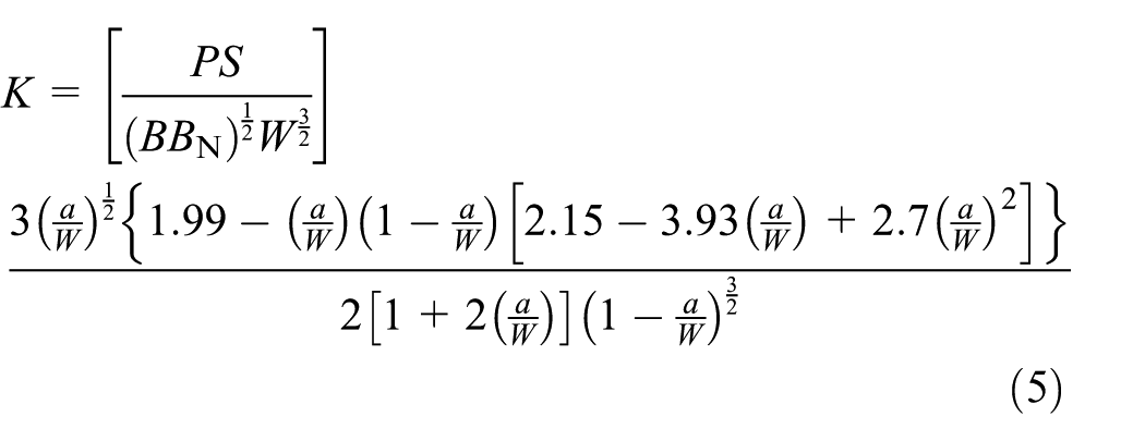
where B and B_N is the specimen thickness and net specimen thickness, respectively. S = 4W is the support span.

Table 5.

Fracture toughness test results for S55C (SE(B) specimen: W = 25 mm, B/W = 0.5).

T (°C)	Specimen ID	1	2	3	4	5	6	μ	Σ
20	a/W	0.51	0.50	0.50	0.50	0.50	0.50	0.50	0.00
	P c (kN)	12.2	10.8	11.7	11.6	12.6	12.7	12.0	0.71
	K c (MPam1/2)	67.7	58.9	63.1	62.6	68.3	68.0	65.4	3.83
	J el (N/mm)	18.6	14.1	16.6	15.9	19.3	19.3	17.6	2.12
	J pl (N/mm)	65.4	40.0	64.3	51.1	62.8	59.7	61.3	9.88
	J c (N/mm)	84.0	54.1	80.9	67.0	82.1	79.0	78.9	11.7
	KJ c (MPam1/2)	144	115	140	129	141	138	141	10.8
	M	55.7	87.8	59.0	71.0	57.9	60.6	59.3	12.2
−45	a/W	0.50	0.50	0.50	0.50	0.50	0.50	0.50	0.00
	P c (kN)	9.70	8.10	9.37	8.73	10.2	9.56	9.47	0.75
	K c (MPam1/2)	52.6	44.2	50.3	47.6	55.5	51.5	50.9	3.96
	J el (N/mm)	12.2	8.26	10.8	9.28	12.7	10.8	10.8	1.69
	J pl (N/mm)	2.16	0.98	1.34	1.76	4.59	1.54	1.65	1.30
	J c (N/mm)	14.4	9.24	12.1	11.0	17.3	12.3	12.5	2.81
	KJ c (MPam1/2)	57.0	46.8	53.3	51.9	64.7	55.1	54.2	5.96
	M	411	636	490	533	339	483	487	102
−85	a/W	(0.50)	(0.50)	0.50	(0.50)	0.50	0.50	0.50	0.00
	P c (kN)	(6.83)	(6.43)	8.05	(6.99)	8.51	7.55	8.05	0.48
	K c (MPam1/2)	(37.3)	(34.9)	43.9	(37.5)	46.3	40.8	43.9	2.76
	J el (N/mm)	(6.70)	(5.06)	8.23	(6.36)	9.17	7.16	8.23	1.01
	J pl (N/mm)	(0)	(0.18)	0.22	(0.17)	0.74	0.48	0.48	0.26
	J c (N/mm)	(6.70)	(5.24)	8.45	(6.53)	9.91	7.64	8.71	1.15
	KJ c (MPam1/2)	(37.3)	(35.5)	44.4	(38.0)	48.1	42.1	44.4	3.02
	M	(1059)	(1333)	825	(1081)	704	917	825	107

Here, μ and Σ are the median and standard deviation of each parameter, respectively. Data in parenthesis indicate K_Ic data that were not used for calculating µ and σ in this table and in the data analysis in the following section.

Table 6.

Fracture toughness test results for SCM440 (SE(B) specimen: W = 25 mm, B/W = 0.5).

T (°C)	Specimen ID	1	2	3	4	5	6	μ	Σ
100	a/W	0.50	0.50	0.50	0.50	0.50	0.50	0.50	0.00
	P c (kN)	15.9	14.6	15.2	15.7	13.8	15.6	15.4	0.80
	K c (MPam1/2)	86.1	78.5	82.4	85.6	74.6	84.2	83.3	4.51
	J el (N/mm)	33.7	27.3	28.6	30.2	23.9	29.1	28.9	3.24
	J pl (N/mm)	90.9	91.3	28.7	143	27.3	247	91.1	82.3
	J c (N/mm)	125	119	57.3	173	51.2	276	120	83.3
	KJ c (MPam1/2)	166	164	117	203	109	259	165	55.8
	M	41.0	43.3	88.9	29.5	100	18.5	41.6	32.7
60	a/W	0.50	0.50	0.50	0.50	0.50	0.50	0.50	0.00
	P c (kN)	15.5	14.4	12.3	14.1	15.0	12.0	14.3	1.43
	K c (MPam1/2)	84.6	78.3	67.1	76.0	81.1	65.3	77.2	7.70
	J el (N/mm)	30.8	25.0	18.3	24.3	27.0	17.3	24.7	5.17
	J pl (N/mm)	59.8	58.6	15.7	51.9	58.1	17.6	55.0	21.1
	J c (N/mm)	90.6	83.6	34.0	76.3	85.1	34.9	79.7	25.9
	KJ c (MPam1/2)	145	143	91.5	135	144	92.7	139	25.9
	M	59.4	64.5	159	71.3	63.5	155	68.0	47.8
20	a/W	0.50	0.50	0.50	0.50	0.50	0.50	0.50	0.00
	P c (kN)	12.2	15.7	13.3	15.4	14.5	14.7	14.6	1.33
	K c (MPam1/2)	65.3	84.4	71.8	83.3	78.1	79.0	78.6	7.26
	J el (N/mm)	17.2	29.7	20.7	28.7	25.0	25.5	25.3	4.77
	J pl (N/mm)	9.83	39.4	19.2	39.3	29.9	36.4	33.2	12.1
	J c (N/mm)	27.0	69.1	39.9	68.0	54.9	61.9	58.5	16.8
	KJ c (MPam1/2)	81.8	129	99.6	128	116	123	120	18.7
	M	213	83.0	143	84.1	105	92.6	98.8	50.6
−55	a/W	0.52	0.51	0.50	0.50	0.50	0.50	0.50	0.01
	P c (kN)	12.1	10.1	10.9	9.49	12.6	12.1	11.5	1.25
	K c (MPam1/2)	69.1	56.7	59.2	50.9	66.8	65.8	62.5	7.00
	J el (N/mm)	18.7	12.5	14.4	11.0	19.6	18.2	16.3	3.59
	J pl (N/mm)	8.98	2.86	3.49	1.01	3.90	3.23	3.36	2.68
	J c (N/mm)	27.7	15.4	17.9	12.0	23.5	21.4	19.7	5.70
	KJ c (MPam1/2)	84.1	62.9	66.0	53.2	73.2	71.4	68.7	10.4
	M	380	416	364	545	281	304	372	94

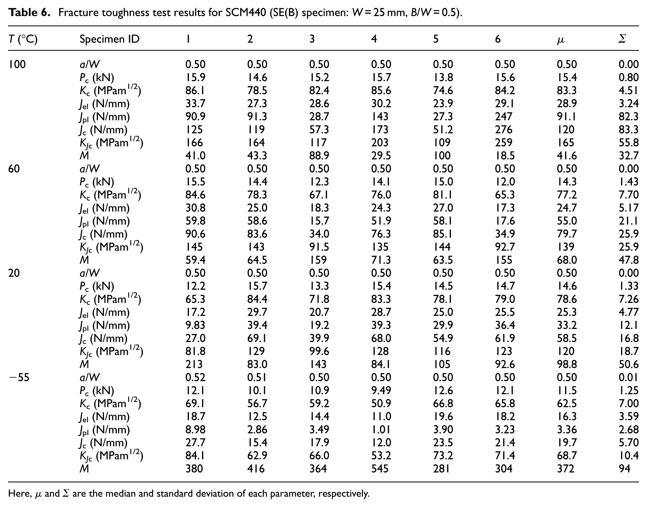
Here, μ and Σ are the median and standard deviation of each parameter, respectively.

J _c is the fracture toughness calculated using equation (6) based on the load P–crack mouth opening displacement V_g diagram (P–V_g diagram) obtained according to ASTM E1921²

$$J_{\mathrm{c}}=J_{\mathrm{el}}+J_{\mathrm{pl}}=\frac{K_{\mathrm{c}}^2(1-{\nu }^2)}{E}+\frac{\eta A_{\mathrm{p}}}{B_{\mathrm{N}}(W-a)}$$

(6)

where area A_p is the plastic component corresponding to the P–V_g diagram and η = 3.667 − 2.199(a/W) + 0.4376(a/W) ² . K_Jc = (EJ_c/(1 − ν²))^1/2, where E is Young’s modulus and ν = 0.3 is Poisson’s ratio. M = (W − a) σ_YS/J_c.

Fracture toughness test results

The test data for both materials obtained at −166°C were the plane–strain fracture toughness K_Ic, defined in ASTM E399 ²³ as P_c/P_Q < 1.1, where P_Q is the cross point of the P–V_g diagram and 95% slope of its linear region. Because this study aims to validate the SDS method in the DBTT region, the test results at −166°C were not included in these tables. Three K_Ic data (specimen id 1, 2, and 4, for which P_c/P_Q < 1.1 and thus J_pl ≈ 0) were observed for S55C at −85°C, and thus, they were excluded in the data analysis. Two data points with M < 30 (specimen id 4 and 6) were obtained for SCM440 at 100°C. Because these two data points showed the stable crack extension to be less than (W – a)/20 and showed cleavage fracture, they were considered valid K_Jc data.

Figure 7(a) and (b) show the relationship between fracture load P_c and tested temperature T for S55C and SCM440, respectively. All data were plotted regardless of whether they belonged to K_Ic or K_Jc or whether they satisfied the ASTM E1921 requirement of M = σ_YS (W − a)/J_c ≥ 30. Figure 8 shows the temperature dependence of the fracture toughness K_Jc or plane–strain fracture toughness K_Ic for S55C and SCM440.

Figure 7.

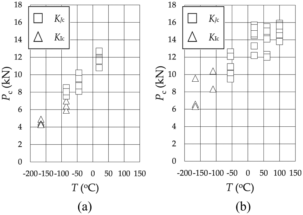
Relationship between fracture load P_c and tested temperature T for (a) S55C and (b) SCM440.

Figure 8.

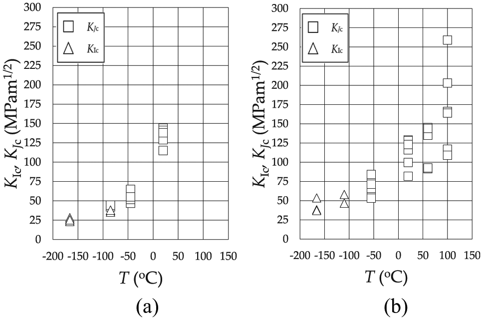
Temperature dependence of fracture toughness K_Jc or K_Ic for (a) S55C and (b) SCM440.

Validation of SDS method

The temperature dependence of P_c was reinterpreted as relationships between P_c and 1/σ_YS for S55C and SCM440 in Figure 9(a) and (b), respectively. Here, P_c for data corresponding to K_Ic was excluded. Considering that S55C showed a clear yield point but SCM440 did not, 0.2% proof stress was commonly used for σ_YS. The straight line in this figure was determined from a linear regression using all data. The experimental data indicated by the marks suggest a clear linear relationship for S55C and a probable linear relationship for SCM440. Thus, a cross-validation method ²⁴ was used to examine the validity of the linear regression.

Figure 9.

Temperature dependence of fracture load P_c reinterpreted as a relationship between P_c and σ_YS⁻¹: (a) clear linear relationship for S55C and (b) probable linear relationship for SCM440.

A polynomial f(x) of highest order Q as defined in equation (7) is assumed, and the sample data set is fitted to this f(x), where x = σ_YS⁻¹. Then, the root-mean-square error (E_RMS) defined in equation (8) is evaluated for the remaining data set of sample number N, where y = P_c. From the combination of the selected sample data set, the minimum, median, and maximum E_RMS were obtained as shown in Table 7. The highest Q is equal to the number of x data minus one; for S55C and SCM440, the number of x data is 3 and 4, so the highest Q is 2 and 3, respectively.

Table 7.

Root-mean-square error E_RMS for fitting the P_c – (1/σ_YS) relationship by polynomial of order Q.

Material	S55C			SCM440
Q	0	1	2	0	1	2	3
Max	2.26	1.31	1.37	2.71	2.35	2.34	2.31
Median	1.75	0.84	0.96	1.94	1.49	1.59	1.72
Min	1.57	0.56	0.72	1.67	1.12	1.08	1.25

According to Table 7, the median E_RMS was minimum for Q = 1 regardless of material, and thus, the linear relationship between P_c and 1/σ_YS was validated for the two materials. This conclusion is supported by a comparison of the fitted f(x) of order Q, where E_RMS is closest to the mean E_RMS in Figure 10(a) and (b)

$$f\left(x\right)=\sum _{q=0}^Q{w}_q{x}^q$$

(7)

$$E_{\mathrm{RMS}}=\sqrt{\sum _{n=1}^N\frac{{(f(x_n)-y_n)}^2}{N}}$$

(8)

Figure 10.

Relationship between P_c and σ_YS⁻¹: linear regression was validated by the cross-validation method for (a) S55C and (b) SCM440.

SDTS method

Derivation of SDTS method

In this study, the SDS method was validated for two materials in a wide temperature range, and the fracture load P_c was shown to be proportional to the inverse of the yield stress σ_YS in the DBTT region. Therefore, if a fracture toughness test is performed at a reference temperature T_r and fracture load P_cr is obtained, then fracture load P_ci at the temperature of interest T_i can be predicted by performing tensile tests at T_r and T_i. If a detailed stress–strain relationship can be obtained for T_i, the fracture toughness could be predicted accurately by running 3D EP-FEA up to the maximum load of P_ci. However, in many cases, tensile tests are performed as check tests, and only the yield and tensile stresses are known.

In the following, a four-step spreadsheet-based method to predict the J_c temperature dependence using the yield stress as tensile test data is proposed and is referred to as the SDTS method. Specifically, a situation is assumed in which the fracture toughness test data (median fracture load P_cr(med) and median of fracture toughness elastic and plastic contributions J_crel(med) and J_crpl(med)), yield stress σ_YSr, and R–O parameters (n_r and σ_0r) at reference temperature T_r are known and the prediction of median fracture toughness J_ci(med) at the temperature of interest T_i is considered. At T_i, only a check tensile test was performed, and thus, R–O parameters are not known and only yield stress σ_YSi is known. By assuming that the difference in R–O exponent n between the two temperatures is small, the SDS method can be applied from an engineering viewpoint.

Step (1)—prediction of P_ci: fracture load at T_i.

P _ci is predicted from P_cr(med) by applying the SDS method, as described by equation (3). Because R–O parameter σ_0i is not known at T_i, yield stresses are used instead as follows

$$P_{\mathrm{ci}}=\frac{{\sigma }_{\mathrm{YSr}}}{{\sigma }_{\mathrm{YSi}}}{P}_{\mathrm{cr}(\mathrm{med})}$$

(9)

Considering that the proposed method is applicable to both materials irrespective of whether they show a clear yield point, 0.2% proof stress was commonly used for σ_YS.

Step (2)—prediction of J_eli: elastic contribution to fracture toughness at T_i.

J _eli can be evaluated immediately by calculating the SIF K_i corresponding to P_ci and using the following equation

$$J_{\mathrm{el}\mathrm{i}}=\frac{(1-{\nu }^2)K_{\mathrm{i}}^2}{E_{\mathrm{i}}}$$

(10)

where E_i and ν are Young’s modulus and Poisson’s ratio of the material, respectively. Because a detailed stress–strain curve is assumed to not be available at T_i, E_i = σ_YSi/0.002 is used to calculate J_eli. ν = 0.3 is always used. In the case of SE(B) specimens, K_i is calculated using the following equation given in ASTM E1921 ²

$$\begin{array}{c}\multicolumn{1}{c}{K_{\mathrm{i}}=\left[\frac{P_{\mathrm{ci}}S}{{\left(B{B}_{\mathrm{N}}\right)}^{\frac{1}{2}}{W}^{\frac{3}{2}}}\right]}\\ \multicolumn{1}{c}{\frac{3{\xi }^{\frac{1}{2}}\{1.99-\left(\xi \right)(1-\xi )(2.15-3.93\xi +2.7{\xi }^2)\}}{2(1+2\xi ){(1-\xi )}^{\frac{3}{2}}}}\end{array}$$

(11)

where ξ = a/W is the ratio of crack length a to the specimen width W, B and B_N are the nominal and net specimen thickness, respectively. S = 4W is the support span.

Step (3)—prediction of J_pli: plastic contribution to fracture toughness at T_i.

For the plastic contribution J_pl, the following Electric Power Research Institution (EPRI) equation ²⁵ was tentatively considered

$$J_{\mathrm{pl}}=\alpha {\epsilon }_0{\sigma }_{0}b{h}_1(\frac{a}{W},n){\left(\frac{P_{\mathrm{c}}}{P_0}\right)}^{n+1}$$

(12)

where ligament length b = W – a; α, σ₀, and n are the R–O parameters; and ε₀ = 0.002. h₁ is a function of a/W and n, which depends on the structure type. P₀ is the reference load given for the structure type of interest. In the case of SE(B) specimens, P₀ for SE(B) specimens is given as

$$P_0=\frac{\mathrm{cB}{b}^2{\sigma }_0}{S}$$

(13)

where span S = 4W and c is a constant specified for a plane–strain or stress condition. By combining these two equations, J_pl for SE(B) specimens is expressed as

$$J_{\mathrm{pl}}=\alpha {\epsilon }_0{\sigma }_{0}b{h}_1(\frac{a}{W},n){\left(\frac{P_{\mathrm{c}}S}{\mathrm{cB}{b}^2{\sigma }_0}\right)}^{n+1}$$

(14)

Because the EPRI J_pl equation is given for limited cases of plane–strain and stress condition, whereas the actual specimens are 3D and are different from these two extreme cases, it was considered that the absolute value of J_pl could not be predicted by the EPRI equation even if the load, specimen dimensions, and R–O parameters were given. However, if the functional shape of the EPRI equations can be used for 3D specimens, the 3D effects will be reflected in h₁ and c in equation (14). If this assumption is accepted, it was considered that the J_pl ratio at the fracture load between temperatures T_r and T_i could be predicted using equation (14) as follows

$$\begin{array}{c}\multicolumn{1}{c}{\frac{J_{\mathrm{pli}}}{J_{\mathrm{plr}}}=\frac{{\alpha }_{\mathrm{i}}{\epsilon }_0{\sigma }_{0\mathrm{i}}b{h}_1(\frac{a}{W},n_{\mathrm{i}}){\left(\frac{P_{\mathrm{ci}}S}{\mathrm{cB}{b}^2{\sigma }_{0\mathrm{i}}}\right)}^{n_{\mathrm{i}}+1}}{{\alpha }_{\mathrm{r}}{\epsilon }_0{\sigma }_{0\mathrm{r}}b{h}_1(\frac{a}{W},n_{\mathrm{r}}){\left(\frac{P_{\mathrm{cr}}S}{\mathrm{cB}{b}^2{\sigma }_{0\mathrm{r}}}\right)}^{n_{\mathrm{r}}+1}}}\\ \multicolumn{1}{c}{=\frac{{\alpha }_{\mathrm{i}}{\sigma }_{0\mathrm{i}}{h}_1(\frac{a}{W},n_{\mathrm{i}}){\left(\frac{P_{\mathrm{ci}}S}{\mathrm{cB}{b}^2{\sigma }_{0\mathrm{i}}}\right)}^{n_{\mathrm{i}}+1}}{{\alpha }_{\mathrm{r}}{\sigma }_{0\mathrm{r}}{h}_1(\frac{a}{W},n_{\mathrm{r}}){\left(\frac{P_{\mathrm{cr}}S}{\mathrm{cB}{b}^2{\sigma }_{0\mathrm{r}}}\right)}^{n_{\mathrm{r}}+1}}}\end{array}$$

(15)

Under another assumption that the temperature dependence of R–O parameters n and α is small in the considered temperature range and by combining equation (9) and replacing σ₀s with σ_YSs, equation (15) can be expressed in a very simple form as follows

$$\frac{J_{\mathrm{pl}i}}{J_{\mathrm{pl}\mathrm{r}}}\approx {\left(\frac{{\sigma }_{\mathrm{YSr}}}{{\sigma }_{\mathrm{YS}i}}\right)}^{2n_{\mathrm{r}}+1}$$

(16)

Using the median test value at T_r, J_pli is finally predicted as

$$J_{\mathrm{pl}i}\approx {\left(\frac{{\sigma }_{\mathrm{YSr}}}{{\sigma }_{\mathrm{YS}i}}\right)}^{2n_{\mathrm{r}}+1}{J}_{\mathrm{plr}(\mathrm{med})}$$

(17)

Step (4)—prediction of J_ci: median fracture toughness at T_i.

Finally, J_ci is predicted as the sum of the predicted elastic and plastic components as follows

$$J_{\mathrm{ci}}=J_{\mathrm{el}\mathrm{i}}+J_{\mathrm{pl}\mathrm{i}}$$

(18)

Validation of SDTS method

The application of the SDTS method to S55C has been explained in detail, in a situation where fracture toughness tests were performed at T_r = –85°C and the median fracture toughness J_ci at temperature of interest T_i = –45°C was predicted.

Specifically, by referring to Table 5, the median fracture load at T_r was obtained as P_cr(med) = 8.05 kN. The median elastic contribution J_elr(med) and plastic contribution J_plr(med) to the median fracture toughness J_c(med) were obtained as 8.23, 0.48, and 8.71 N/mm, respectively. The stress–strain relationship is known at T_r, with yield stress (0.2% proof stress in this method) σ_YSr = 561.5 MPa, and R–O exponent n_r = 4.86 is obtained from Table 3. Here, a situation in which the tensile test performed at the temperature of interest T_i = –45°C was a check test, that is, the yield stress σ_YSi = 474.5 MPa is known but the R–O exponent is unknown, is considered. Table 8 presents the spreadsheet inputs and the predicted results for this case:

• Step (1). First, by applying equation (9), the fracture load at T_i was predicted as P_ci = 9.53 kN. This was only 0.64% different from the median of experimental results, which is 9.47 kN, as listed in Table 5.

• Step (2). This naturally leads to an acceptable J_eli prediction using the SE(B) SIF equation given in equation (11).

• Thus, J_eli calculated from equations (10) and (11) shows a difference of −6.48% from the median test value of 10.8 N/mm. In this calculation, Young’s modulus at T_i was calculated as E_i = σ_YSi/0.002, and Poisson’s ratio of ν = 0.3 was used.

• Step (3). Next, the plastic contribution J_pli was predicted using equation (17). Table 8 shows that this prediction of 2.92 N/mm was comparable with the median test value of 1.65 N/mm.

• Step (4). Finally, the fracture toughness J_ci at T_i was predicted by equation (18). J_ci = J_eli+J_pli= 13.0 N/mm differed by only 4.00% from the median test value of 12.5 N/mm.

Table 8.

Prediction result for S55C for reference temperature T_r of −85°C and temperatures of interest T_i of −45°C and 20°C.

Step		T r (°C)	Ti (°C)		Note
		–85	–45	20
	n	4.86
	σYS (MPa)	561.5	474.5	381.5
(1)	P ci (kN)		9.53	11.8	Prediction by equation (9)
	P c(med) (kN)	8.05	9.47	12.0	Median of experiments
	Difference (%)		0.64	−1.67
(2)	J eli (N/mm)		10.1	19.4	Prediction by equations (10) and (11)
	J el(med) (N/mm)	8.23	10.8	17.6	Median of experiments
	Difference (%)		−6.48	10.5
(3)	J pli (N/mm)		2.92	30.2	Prediction by equation (17)
	J pl(med) (N/mm)	0.48	1.65	61.3	Median of experiments
	Difference (%)		76.8	−50.6
(4)	J ci (N/mm)		13.0	49.6	Prediction by equation (18)
	J c(med) (N/mm)	8.71	12.5	78.9	Median of experiments
	Difference (%)		4.00	−37.1

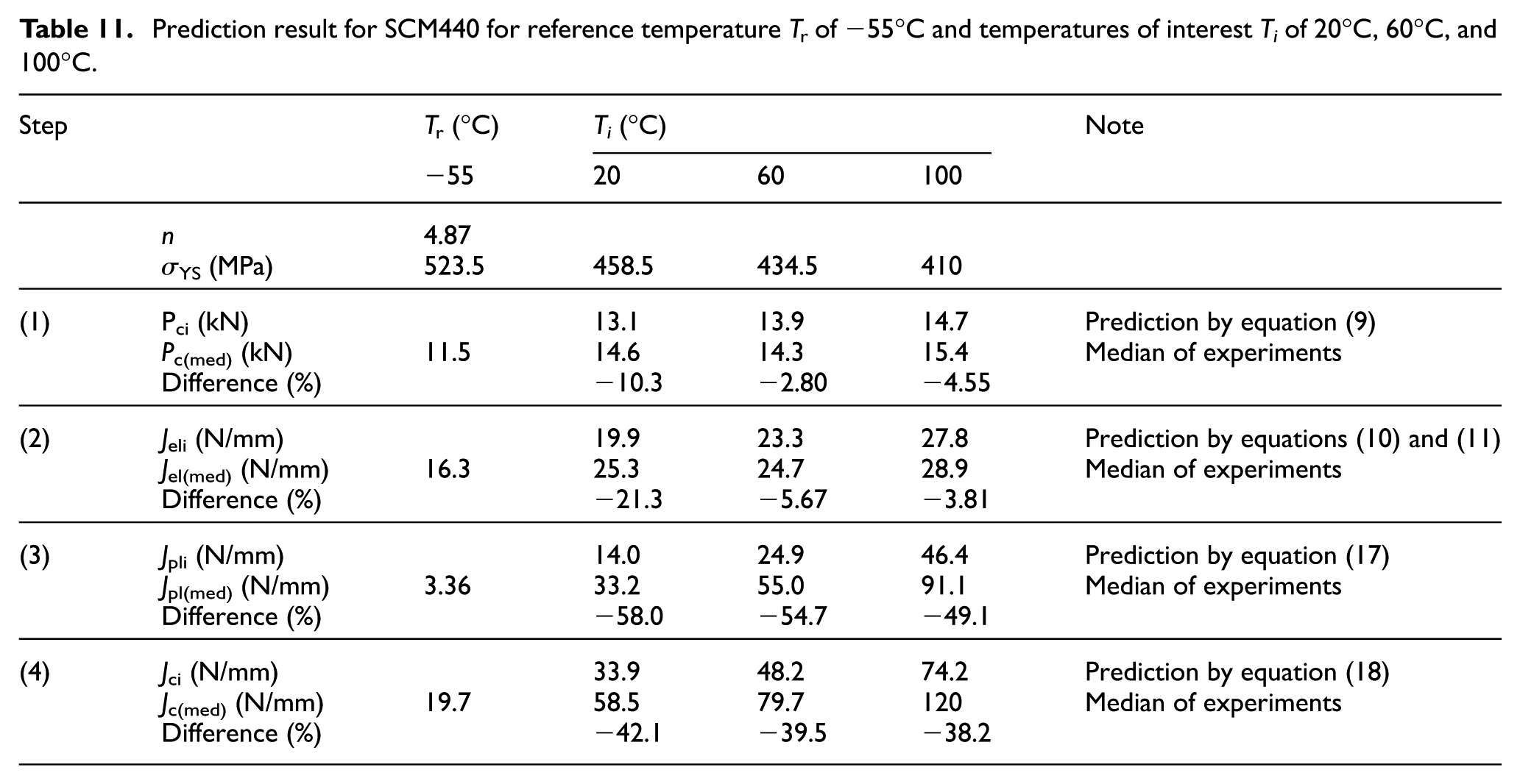
Tables 8–10 show the other temperature combination results for S55C. Similarly, Tables 11–14 show the results for SCM440. The average difference (absolute) between the predicted and mean test J_c values for 18 cases was 22.1%. The maximum observed difference for S55C was −50.4% for T_r = –45 and T_i = 20°C, and the minimum difference was 4.00% for T_r = –85 and T_i = –45°C. Generally, the prediction difference was small when T_r > T_i because J_pli is sensitive to P_ci change at higher temperatures.

Table 9.

Prediction result for S55C for reference temperature T_r of −45°C and temperatures of interest T_i of −85°C and 20°C.

Step		T r (°C)	Ti (°C)		Note
		−45	−85	20
	n	5.21
	σ YS (MPa)	474.5	561.5	381.5
(1)	P ci (kN)		8.00	11.8	Prediction by equation (9)
	P c(med) (kN)	9.47	8.05	12.0	Median of experiments
	Difference (%)		−0.64	−1.67
(2)	J eli (N/mm)		6.02	19.2	Prediction by equations (10) and (11)
	J el(med) (N/mm)	10.8	8.23	17.6	Median of experiments
	Difference (%)		−26.8	9.09
(3)	J pli (N/mm)		0.21	19.9	Prediction by equation (17)
	J pl(med) (N/mm)	1.65	0.48	61.3	Median of experiments
	Difference (%)		−56.3	−67.5
(4)	J ci (N/mm)		6.23	39.1	Prediction by equation (18)
	J c(med) (N/mm)	12.5	8.71	78.9	Median of experiments
	Difference (%)		−28.5	−50.4

Table 10.

Prediction result for S55C for reference temperature T_r of 20°C and temperatures of interest T_i of −85°C and −45°C.

Step		T r (°C)	Ti (°C)		Note
		20	−85	−45
	n	5.19
	σ YS (MPa)	381.5	561.5	474.5
(1)	P ci (kN)		8.12	9.61	Prediction by equation (9)
	P c(med) (kN)	12.0	8.05	9.47	Median of experiments
	Difference (%)		0.86	1.51
(2)	J eli (N/mm)		6.20	10.3	Prediction by equations (10) and (11)
	J el(med) (N/mm)	17.6	8.23	10.8	Median of experiments
	Difference (%)		−24.6	−4.63
(3)	J pli (N/mm)		0.75	5.12	Prediction by equation (17)
	J pl(med) (N/mm)	61.3	0.48	1.65	Median of experiments
	Difference (%)		56.9	210
(4)	J ci (N/mm)		6.95	15.4	Prediction by equation (18)
	J c(med) (N/mm)	78.9	8.71	12.5	Median of experiments
	Difference (%)		−20.2	23.2

Table 11.

Prediction result for SCM440 for reference temperature T_r of −55°C and temperatures of interest T_i of 20°C, 60°C, and 100°C.

Step		T r (°C)	Ti (°C)			Note
		−55	20	60	100
	n	4.87
	σ YS (MPa)	523.5	458.5	434.5	410
(1)	Pci (kN)		13.1	13.9	14.7	Prediction by equation (9)
	P c(med) (kN)	11.5	14.6	14.3	15.4	Median of experiments
	Difference (%)		−10.3	−2.80	−4.55
(2)	J eli (N/mm)		19.9	23.3	27.8	Prediction by equations (10) and (11)
	J el(med) (N/mm)	16.3	25.3	24.7	28.9	Median of experiments
	Difference (%)		−21.3	−5.67	−3.81
(3)	J pli (N/mm)		14.0	24.9	46.4	Prediction by equation (17)
	J pl(med) (N/mm)	3.36	33.2	55.0	91.1	Median of experiments
	Difference (%)		−58.0	−54.7	−49.1
(4)	J ci (N/mm)		33.9	48.2	74.2	Prediction by equation (18)
	J c(med) (N/mm)	19.7	58.5	79.7	120	Median of experiments
	Difference (%)		−42.1	−39.5	−38.2

Table 12.

Prediction result for SCM440 for reference temperature T_r of 20°C and temperatures of interest T_i of −55°C, 60°C, and 100°C.

Step		T r (°C)	Ti (°C)			Note
		20	−55	60	100
	n	4.77
	σ YS (MPa)	458.5	523.5	434.5	410
(1)	P ci (kN)		12.8	15.4	16.3	Prediction by equation (9)
	P c(med) (kN)	14.6	11.5	14.3	15.4	Median of experiments
	Difference (%)		11.2	7.69	5.84
(2)	J eli (N/mm)		16.5	28.9	34.4	Prediction by equations (10) and (11)
	J el(med) (N/mm)	25.3	16.3	24.7	28.9	Median of experiments
	Difference (%)		1.23	17.1	19.0
(3)	J pli (N/mm)		8.22	58.5	108	Prediction by equation (17)
	J pl(med) (N/mm)	33.2	3.36	55.0	91.1	Median of experiments
	Difference (%)		145	6.34	18.3
(4)	J ci (N/mm)		24.7	87.4	142	Prediction by equation (18)
	J c(med) (N/mm)	58.5	19.7	79.7	120	Median of experiments
	Difference (%)		25.8	9.67	18.5

Table 13.

Prediction result for SCM440 for reference temperature T_r of 60°C and temperatures of interest T_i of −55°C, 20°C, and 100°C.

Step		T r (°C)	Ti (°C)			Note
		60	−55	20	100
	n	5.04
	σ YS (MPa)	434.5	523.5	458.5	410
(1)	P ci (kN)		11.8	13.5	15.1	Prediction by equation (9)
	P c(med) (kN)	14.3	11.5	14.6	15.4	Median of experiments
	Difference (%)		2.61	−7.51	−1.94
(2)	J eli (N/mm)		14.1	21.0	29.4	Prediction by equations (10) and (11)
	J el(med) (N/mm)	24.7	16.3	25.3	28.9	Median of experiments
	Difference (%)		−13.4	−16.8	1.73
(3)	J pli (N/mm)		6.99	30.3	105	Prediction by equation (17)
	J pl(med) (N/mm)	55.0	3.36	33.2	91.1	Median of experiments
	Difference (%)		108	−8.65	14.8
(4)	J ci (N/mm)		21.1	51.3	134	Prediction by equation (18)
	J c(med) (N/mm)	79.7	19.7	58.5	120	Median of experiments
	Difference (%)		7.11	−12.2	11.7

Table 14.

Prediction result for SCM440 for reference temperature Tr of 100°C and temperatures of interest Ti of −55°C, 20°C, and 60°C.

Step		T r (°C)	Ti (°C)			Note
		100	−55	20	60
	n	5.14
	σ YS (MPa)	410	523.5	458.5	434.5
(1)	P ci (kN)		12.1	13.8	14.5	Prediction by equation (9)
	P c(med) (kN)	15.4	11.5	14.6	14.3	Median of experiments
	Difference (%)		5.22	−5.48	1.40
(2)	J eli (N/mm)		14.7	21.9	25.7	Prediction by equations (10) and (11)
	J el(med) (N/mm)	28.9	16.3	25.3	24.7	Median of experiments
	Difference (%)		−9.82	−13.4	4.05
(3)	Jpli (N/mm)		5.79	25.8	47.3	Prediction by equation (17)
	Jpl(med) (N/mm)	91.1	3.36	33.2	55.0	Median of experiments
	Difference (%)		72.2	−22.3	−13.9
(4)	J ci (N/mm)		20.5	47.7	73.0	Prediction by equation (18)
	J c(med) (N/mm)	120	19.7	58.5	79.7	Median of experiments
	Difference (%)		4.12	−18.4	−8.32

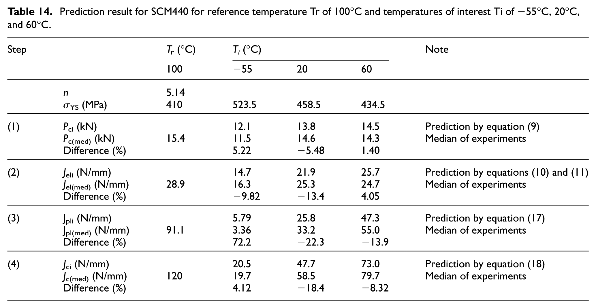
A similar tendency was observed for SCM440. The maximum observed difference was −42.1% for T_r = –55°C and T_i = 20°C, and the minimum difference was 4.12% for T_r = 100°C and T_i = –55°C.

In summary, the prediction discrepancy for these 18 cases ranged from −50.4% to +25.8%, and the average absolute difference was 22.1%. Considering the large scatter in J_c values, the proposed SDTS method seems to achieve prediction accuracy that is sufficient from an engineering viewpoint.

Discussion

The significance of the SDTS method is that it will enable design engineers and practitioners to predict the J_c temperature dependence in minimal time without requiring costly fracture toughness tests. Specifically, the SDTS method is advantageous because (1) it does not require preliminary tests to determine a suitable fracture toughness test temperature (cf. MC approach requires preliminary tests such as the Charpy impact test to select the fracture toughness test temperature so that this temperature is close to the desired reference temperature T₀) and an arbitrary temperature can be selected as the reference temperature T_r, and (2) J_c at the temperature of interest T_i can be predicted by a simple spreadsheet calculations.

The disadvantage of the SDTS method is that it requires tensile test results at T_r and T_i; specifically, it requires the R–O exponent n and σ_YS at T_r and σ_YS at T_i. This means that check tensile test is not sufficient and a detailed stress–strain relationship is necessary at T_r. However, this disadvantage seems allowable because tensile test specimens are small compared with fracture toughness test specimens and they show small scatter; therefore, two tests are usually enough.

Moreover, there exist an equation based on Considere’s construction to estimate the R–O exponent n from the nominal yield and tensile stress σ_YS and σ_B obtained from tensile tests as following ²⁶

$$\frac{{\sigma }_{\mathrm{B}}}{{\sigma }_{\mathrm{YS}}}={\left(\frac{\frac{1}{n}}{0.002+\frac{{\sigma }_{\mathrm{YS}}}{E}}\right)}^{\frac{1}{n}}\exp \left(\frac{-1}{n}\right)$$

(19)

Equation (19) estimated n within a range of −5.3% to +21.7% for S55C compared with the values listed in Table 3, and −5.5% to +2.6% for SCM440 compared with the values listed in Table 4. These results are acceptable, and in cases where a detailed tensile test to obtain a stress–strain relationship cannot be performed, this estimate will help.

The significance and advantages of the SDTS method compared with the ASTM E1921 MC approach are that it enables better J_c prediction at high temperature using low-temperature J_c data. For example, assume that the only data available for SCM440 were tested at −55°C; its SDTS reference temperature is T_r = –55°C and MC reference temperature is T₀ = –8.9°C. Because|T₀—T_r| = 46.1°C, this test was valid. Figure 11 shows the predictions performed using the two methods. The MC approach gave a non-conservative prediction for temperatures higher than 20°C, whereas the SDTS approach predicted K_Jc around the median value for all temperatures of interest.

Figure 11.

Comparison of fracture toughness K_Jc temperature dependence prediction from test data obtained at −55°C for SCM440 by SDTS method and by ASTM E1921 MC method. The SDTS method showed better prediction than the MC method at temperatures higher than the test temperatures.

Figure 11 shows that the effort of obtaining supplemental tensile test data at T_i, which is required in the SDTS method, is worthwhile because of the resulting large improvement in K_Jc prediction accuracy. The SDTS method is expected to solve the problem of improving the prediction for relatively high temperatures that is faced in the MC approach. ¹

The SDTS method was validated for application to the SE(B) specimen in this study. Because the EPRI J_pl functional form for other fracture toughness test specimen types is similar, the SDTS method is expected to be useful for other specimen types. Future studies should validate the SDTS method for other specimen types. In these future studies, if J_pl equations are developed for fracture toughness specimens that consider 3D size effects, improvement in the accuracy of J_c temperature dependence prediction is expected. Development of these equations is also our future work.

Conclusion

In this work, a spreadsheet-based method called the SDTS method was proposed to predict the temperature dependence of fracture toughness J_c in the DBTT region. Necessary data are fracture toughness test data (P_c, J_c with its components J_el and J_pl) and R–O exponent n and σ_YS at reference temperature T_r and σ_YS at the temperature of interest T_i to predicted J_c. The physical basis of the SDTS method is that the fracture stress for slip-induced cleavage fracture is temperature independent. The SDTS method was validated in a wide temperature range of −85°C to +20°C for S55C and −55°C to +100°C for SCM440. The prediction discrepancy for these 18 cases ranged from −50.4% to +25.8% and the average absolute difference was 22.1%. In particular, in cases for predicting J_c at temperatures higher than the lowest temperature of −55°C for SCM440, the SDTS method predicted J_c more realistically than the ASTM E1921 MC approach, even in a case of T_i = 100°C. Although the SDTS method requires additional tensile test data compared with the MC approach, the prediction improvement at high temperatures seems beneficial because the mass and time required for additional tensile tests are admissible.