Development and validation of wear models by using innovative three-dimensional laser scanners

Abstract

One of the main problems in railway and tramway systems, both dynamically (safety, comfort etc.) and economically (planning of maintenance interventions, reduction of wheel and rail lifetime etc.), is represented by the wear of wheel and rail profiles, due to the wheel–rail interaction. The profile’s shape variation caused by wear influences the dynamic behaviour of the vehicle and, in particular, the wheel–rail contact conditions. Hence, nowadays, one of the most important topics in the railway field is the development of reliable wear models to predict profiles evolution, together with the use of more efficient and accurate measuring instruments for the model validation and the rolling components inspection. In this context, the aim of this research work is the development and the validation of wear models, using experimental data acquired through an innovative measuring instrument based on noncontact three-dimensional laser scanning technology. The tramway line of the city of Florence, characterized by very narrow curves and critical in terms of wear, has been chosen as a reference test case. Moreover, the inspection procedures currently adopted on this line for the maintenance plan are based only on classical two-dimensional contact measurement systems, not so accurate for a complete wear assessment. Therefore, the introduction of a new three-dimensional laser scanning technology may have a great impact on the maintenance management of the line.

Introduction

The wear at the wheel–rail interface is a crucial aspect in the tramway field. Wear causes changes in wheel and rail profiles with a great effect on vehicle dynamics and on running stability, leading to performance decay and a less comfortable ride. ¹ Therefore, the original profiles must be periodically reconstructed by means of turning or grinding, in order to guarantee the running under safe condition, with a consequent increase in the maintenance costs. For these reasons, the development of reliable wear models represents a powerful tool both for the vehicle design and for the maintenance planning.^2–5

Because of the importance of rail and wheel conditions, their health status is constantly monitored by means of different measuring instruments. Currently, many digital wear measurement methods exist, and in general, they can be classified as direct and indirect.^6,7 Direct methods are used when the direct access to the worn surface is possible optically or by contact, and while when the access is impossible, indirect methods are used. The latter methods do not measure wear directly but they measure specific quantities which are caused by wear (e.g. heat, noise, vibration etc.) and which can be put in relationship with wear, by means of analytic formulas.^6,7

Direct methods range from visual inspection and two-dimensional (2D) contact profilometer to the most recent and innovative 2D/3D optical scanners. Currently, 2D wear measurements are the most used to check wheel and rail wear condition. They use a mechanical sensing probe (2D contact profilometer^6,8–10) or a laser beam (2D optical profilometer ¹ ) to detect a set of reference parameters which are representative of the wear status of the entire wheel and rail profiles geometry. However, most of them do not allow an accurate assessment of specific three-dimensional (3D) wear phenomena such as corrugation and plastic deformations. The most recent devices exploit 3D laser systems to detect wheel and rail surfaces in terms of Cartesian coordinates and polygonal meshes and, thanks to the continuous improvement of laser scanning technology, a higher degree of accuracy and efficiency can be reached, allowing a more complete analysis of the wear conditions over the whole component surfaces.^6,11–13 Thanks to their great versatility, reliability and accuracy; the use of these measuring instruments is highly suggested especially with a complex shape sample. Furthermore, some 3D optical scanners have the advantage of being portable, allowing to scan undercuts and complex geometries in a simple way^8,14 and without dismounting the components from their exercise environment. This way, it is possible to generate a full 3D digital model of the specimen and to accurately compare it to the unworn geometry, getting the final 3D distribution of material removed by wear. The resulting 3D wear maps allow also the measurement of several wear parameters, which would be unappreciable by 2D measurements. Thus, a complete scenario of the wear phenomenon can be achieved.

Together with the continuous improvement in monitoring instruments and techniques, the development of efficient wear models able to predict rail and wheel profile evolution is a powerful tool to better manage wheel and rail damages and optimize maintenance interventions.^15–17

The proposed wear model, based on the so-called T-gamma approach according to Braghin et al. ¹⁸ and Lewis and Dwyer-Joyce ¹⁹ in its local version, is able to simultaneously evaluate the wear progress both on the rail and on the wheel (see Figure 1). The T-gamma approach makes use of an experimental law to directly connect the power dissipated at the contact to the amount of material removed by wear.

Figure 1.

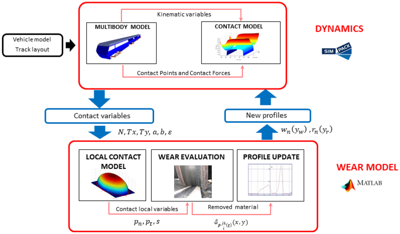
Model general architecture.

The whole model is made up of two reciprocally interacting blocks. In the dynamics block, the dynamical analysis is carried out: a 3D multibody model of the vehicle, implemented in Simpack environment, interacts online, creating a loop, with the global contact model. The latter is based on an efficient algorithm developed by University of Florence^20,21 in the previous years concerning the contact points detection, while the contact forces (normal and tangential) and the global creepages on the contact patch are calculated through the Hertz and Kalker global theories.^22,23 In the second block, the wear evolution is calculated by means of a wear model, entirely implemented in MATLAB and based on a local contact model (the Kalker’s ²² FASTSIM algorithm) which evaluates local pressures and sliding inside the contact patch. Starting from the outputs of the local contact model, the material removed by wear is estimated through an experimental law linking the volume of removed material to the friction power produced by the tangential contact pressures, following the so-called T-gamma approach. ¹⁸ The worn profiles of wheel and rail are obtained by subtracting the worn material from the wheel and rail old profiles and then are sent back to the dynamics block as input of the vehicle model, to go on with the next discrete step of the loop. Therefore, the evolution of the wheel and rail geometry is described through intermediate profiles. An appropriate profile update strategy, based on the distance travelled by the vehicle and the tonnage burden on the track, has been developed taking into account the different time scales characterizing the wear evolution of wheel and rail.

Although the proposed model is capable of calculating both the wheel and the rail wear, in this first step of the project, the focus will be only on the rail, and an accurate validation of the proposed approach will be carried out against experimental rail wear data acquired using a new noncontact portable metrological 3D laser scanner on a curved section of the Florence tramway line. ¹¹ The wear trend numerically evaluated in terms of 2D rail profiles will be compared to the experimental one, and consequently to the 3D wear maps of the worn rails. For the sake of completeness, the wear reference parameters acquired by the classical 2D contact profilometer (currently used in the Florence tramway line) will be also considered to get a more robust validation of the proposed model.

Wear model layout

The wear model (see Figure 1) is able to evaluate the wear progress both on the wheel and on the rail simultaneously. It is made up of two separate blocks that mutually interact: the dynamics block where the dynamical analysis is carried out and the wear model block for the wear evaluation.

Dynamics

The dynamic block consists of the multibody model of the vehicle (built in Simpack Rail environment) and the global contact model that interact online during the dynamical simulations. For this work, a 3D global contact model developed by the authors in previous works^20,21 is exploited to achieve better accuracy and reliability, especially concerning the contact point detection. The contact model calculates the contact forces in the normal and tangential direction and the global creepages on the contact patch through Hertz and Kalker global theories for each detected contact points at each time integration step.^20,21 The global contact variables are passed to the multibody model in order to carry on the simulation of the vehicle dynamics. The tramway track and the multibody model of the considered vehicle are the main inputs of the dynamic block. More particularly, the considered track is the Tram Line 1 of the city of Florence (see Figure 2). The vehicle, which provides passenger service on the considered line, is a 100% low floor independent wheels and articulated tram, built and designed by Hitachi Rail Italy on Sirio platform. It is composed of three bogies, two motors and one trailer, and five coaches, two motors with cabin, one trailer and two hanging (see Figure 3). The wheelbase is 1700 mm and the bogies are equipped with elastic, 660 mm diameter tired wheels with UNI3332 profile, running on a 60R2 rail profile. The adopted suspension system is a two-stage type with the primary suspension fitted with rubber elements and the secondary one consisting of a double coaxial helical spring. The main vehicle characteristics are shown in Table 1.

Figure 2.

Florence Tramway Line 1.

Figure 3.

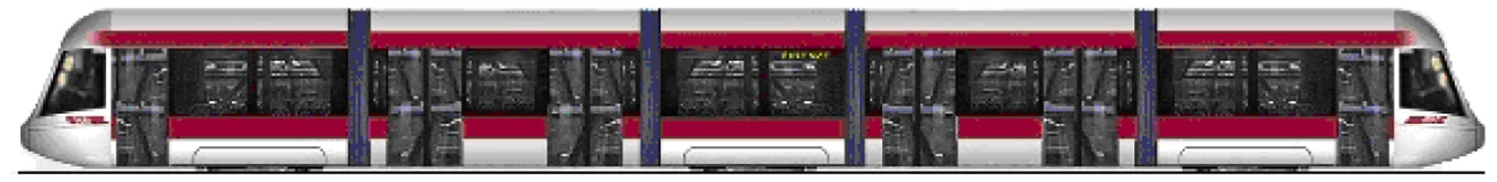
Tram vehicle Sirio.

Table 1.

Main vehicle dimensions.

Vehicle overall length	32,030 mm
Width	2400 mm
Height	3414 mm
Floor height from t.o.r.	350 mm
Wheel arrangement	Bo-2-Bo
Bogie wheelbase	1700 mm
Wheel diameter	660 mm

The multibody model built in Simpack Rail environment is made up of rigid bodies (coaches, drop axle for low floor, motors and gearbox) connected by means of appropriate elastic and damping elements. The primary suspensions are two appropriate spring-damper elements and connect the drop axle to the bogie frame, while the secondary suspensions connect the bogies to the coaches (see Figure 4).

Figure 4.

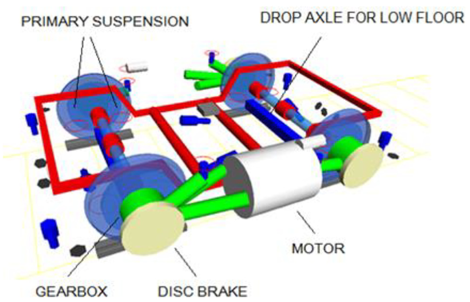
Multibody model of Sirio bogie.

Wear model

The wear model consists of three distinct phases (see Figure 1). In the first one, the local contact model, based on Hertz local theory and on simplified Kalker’s ²² algorithm FASTSIM, starting from the global contact variables calculated by the multibody simulation (global normal and tangential forces, global creepages and contact patch dimensions), evaluates the local contact variables (contact pressures $p_n$ , ${\mathbf{p}}_{\mathrm{t}}$ and local slip $\mathbf{s}$ within every discretization point of the contact patch) and divides the contact patch into adhesion area and creep area. One can refer to literature for a more detailed description of the FASTSIM algorithm. ²²

At this preliminary step of the research activity, the authors have followed the T-gamma approach for the wear evaluation according to Braghin et al. ¹⁸ and Lewis and Dwyer-Joyce. ¹⁹ It makes use of an experimental law to directly connect the power dissipated at the contact (measured by the Wear Index $I_W$ ) to the amount of material removed by wear (measured by the Wear Rate $K_W$ ).

This experimental relationship ¹⁸ has been obtained using two rolling twin discs of R8T steel for the wheel and UIC60 900A widely used in European and Italian network, and it allows to evaluate the specific volume of removed material on wheel and rail (expressed in mm³/(m mm²)) ${\delta }_{P_{\mathrm{wi}(t)}^j}(x,y)$ and ${\delta }_{P_{\mathrm{ri}(t)}^j}(x,y)$ (x and y indicate the coordinates of a generic point inside the contact patch) associated to the ith contact points $P_{\mathrm{wi}}^j(t)$ and $P_{\mathrm{ri}}^j(t)$ on the jth wheel and rail pair for unit of distance travelled by the vehicle (in m) and for unit of surface (in mm²). Moreover, the wear index $I_W$ (a measure of frictional power dissipated at the contact for unit of area and normalized by the vehicle velocity), expressed in N/mm², is evaluated considering the local tangential contact pressure ${\mathbf{p}}_{\mathrm{t}}$ (as calculated in Kalker^22,24) and creepages $\mathbf{s}$

$$I_W={\mathbf{p}}_t•\mathbf{s}/V$$

(1)

where V is the vehicle longitudinal speed. The wear index can be experimentally ¹⁸ correlated to the wear rate $K_W$ , which is the mass of removed material (expressed in μg/(m mm²)) for unit of distance travelled by the vehicle and for unit of surface. The experimental relationship between $K_W$ and $I_W$ is the following (see also Figure 5)

$$K_W\left(I_W\right)=\{\begin{array}{c}5.3^{*}{I}_w\hfill \\ \multicolumn{1}{c}{55.1}\\ \multicolumn{1}{c}{61.9^{*}{I}_W-4723.7}\end{array}\begin{array}{c}{I}_W<10.4\hfill \\ \multicolumn{1}{c}{10.4<I_W<77.2}\\ \multicolumn{1}{c}{I_W>77.2}\end{array}$$

(2)

Figure 5.

Wear rate trend.

The law above also includes the fact that a big part of the frictional power dissipated at the contact transforms into frictional heat. In fact, the frictional power dissipated at the contact is directly correlated by the heuristic wear law to the material removed by wear measured experimentally. Consequently, only the part of the frictional power involved in the wear process is considered by the law, and there is no risk of overestimating the wear on the contact surfaces.

Once the wear rate $K_W(I_W)$ is known (the same both for the wheel and for the rail), the specific volume of removed material on the wheel and on the rail (for unit of distance travelled by the vehicle and for unit of surface) can be calculated (expressed in mm³/(m mm²))

$$\begin{array}{c}{\delta }_{P_{\mathrm{wi}\left(t\right)}^j}(x,y)=K_W\left(I_W\right)\frac{1}{\rho }\hfill \\ {\delta }_{P_{\mathrm{ri}(t)}^j}(x,y)=K_W\left(I_W\right)\frac{1}{\rho }\hfill \end{array}$$

(3)

where $\rho$ is the material density.

After the worn material evaluation, wheel and rail profiles require to be updated prior to be used as the input of the next discrete step of the process. Some previous integration and average operations lead to the calculation of the average wear quantities ${\overline{\mathrm{\Delta }}}^w(s_w)$ and ${\overline{\mathrm{\Delta }}}^r(s_r)$ (expressed in mm).

Longitudinal integration

All the wear contributions inside the contact patch are summed along the longitudinal direction and this quantity is averaged over the whole longitudinal development of the wheel and of the rail (by means of the factors $1/2\pi w(y_{\mathrm{wi}}^j)$ and $1/1l_{\mathrm{track}}{l}_{\mathrm{track}}$ )

$$\begin{array}{c}\frac{1}{2\pi w\left(y_{\mathrm{wi}}^j\right)}\underset{-a(y)}{\overset{+a(y)}{\int }}{\delta }_{P_{\mathrm{wi}}^j(t)}(x,y)\mathrm{dx}={\delta }_{P_{\mathrm{wi}}^j(t)}^{\mathrm{tot}}\left(y\right)\hfill \\ \frac{1}{l_{\mathrm{track}}}\underset{-a(y)}{\overset{+a(y)}{\int }}{\delta }_{P_{\mathrm{ri}}^j(t)}(x,y)\mathrm{dx}={\delta }_{P_{\mathrm{ri}}^j(t)}^{\mathrm{tot}}\left(y\right)\hfill \end{array}$$

(4)

where $w(y_{\mathrm{wi}}^j)$ is the wheel radius evaluated in $y_{\mathrm{wi}}^j$ and $l_{\mathrm{track}}$ is the length of the simulated curve section.

Track integration

This integration over the track length adds all the wear contributions coming from the dynamic simulation to calculate the depth of removed material (in mm = mm³/mm²) on wheel and rail

$$\begin{array}{c}\underset{T_{\mathrm{in}}}{\overset{T_{\mathrm{end}}}{\int }}{\delta }_{P_{\mathrm{wi}}^j(t)}^{\mathrm{tot}}\left(y\right)V\left(t\right)\mathrm{dt}\approx \underset{T_{\mathrm{in}}}{\overset{T_{\mathrm{end}}}{\int }}{\delta }_{P_{\mathrm{wi}}^j(t)}^{\mathrm{tot}}(s_w-{\mathrm{s}}_{\mathrm{wi}}^{\mathrm{cj}}\left(t\right))V\left(t\right)\mathrm{dt}={\mathrm{\Delta }}_{P_{\mathrm{wi}}^j}\left(s_w\right)\hfill \\ \underset{T_{\mathrm{in}}}{\overset{T_{\mathrm{end}}}{\int }}{\delta }_{P_{\mathrm{ri}}^j(t)}^{\mathrm{tot}}\left(y\right)V\left(t\right)\mathrm{dt}\approx \underset{T_{\mathrm{in}}}{\overset{T_{\mathrm{end}}}{\int }}{\delta }_{P_{\mathrm{ri}}^j(t)}^{\mathrm{tot}}(s_r-{\mathrm{s}}_{\mathrm{ri}}^{\mathrm{cj}}\left(t\right))V\left(t\right)\mathrm{dt}={\mathrm{\Delta }}_{P_{\mathrm{ri}}^j}\left(s_w\right)\hfill \end{array}$$

(5)

The natural abscissas $s_w$ and $s_r$ of the curves $w(y_w)$ and $r(y_r)$ have been considered to have a better accuracy in the calculation of the worn profiles, especially in the flange zone and in the rail flank where the slope is steeper (see Figure 6).

Figure 6.

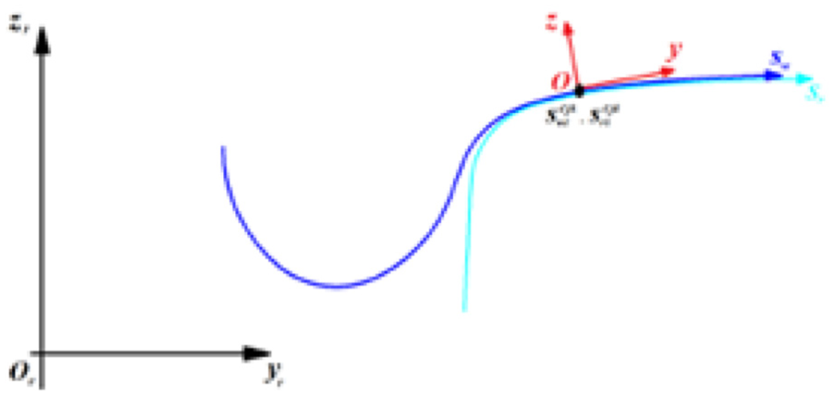
Normal abscissa for the wheel profile.

Sum on the contact points

All the wear contributions of each contact point are summed as follows

$$\begin{array}{c}\sum _{i=1}^{N_{\mathrm{PDC}}}{\mathrm{\Delta }}_{P_{\mathrm{wi}}^j}\left(s_w\right)={\mathrm{\Delta }}_j^w\left(s_w\right)\hfill \\ \sum _{i=1}^{N_{\mathrm{PDC}}}{\mathrm{\Delta }}_{P_{\mathrm{ri}}^j}\left(s_r\right)={\mathrm{\Delta }}_j^r\left(s_r\right)\hfill \end{array}$$

(6)

where $N_{\mathrm{PDC}}$ is the maximum number of contact points of each wheel and of each single rail, respectively. The number of contact points that appear during the dynamic simulation changes with time and it has been assumed that the contribution to wear associated to the fictitious points is zero.

Sum on the right and left wheel–rail pair to evaluate rail wear

The sum on right and left vehicle wheel–rail pairs is calculated to properly get the total rail wear

$$\sum _{j\in \mathrm{left}/\mathrm{right}\mathrm{wheel}}^{N_w}{\mathrm{\Delta }}_j^r\left(s_r\right)={\mathrm{\Delta }}_{l/r}^r\left(s_r\right)$$

(7)

where $N_w$ is the number of vehicle wheels. This operation is not required for the calculation of wheel wear.

Scaling

Since normally travelled distances of thousands of kilometres are needed to obtain measurable wear effects, an appropriate scaling procedure is required to reduce the simulated track length with a consequent lighter computational effort.

Furthermore, the wheels wear out much faster than the rails. Consequently, it is necessary to implement different strategies to update the wheel and rail profiles: the total mileage $k{m}_{\mathrm{tot}}$ travelled by the vehicle is considered for the wheel, which is then subdivided into constant steps of length $k{m}_{\mathrm{step}}$ ; on the contrary, for the rail update, the total tonnage burden on the track $M_{\mathrm{tot}}$ (and then the total number $N_{\mathrm{tot}}$ of vehicle running on the line) is taken into account (see Figure 7). As in the wheel case, the total number $N_{\mathrm{tot}}$ of vehicle operating on the line is subdivided into constant steps equal to $N_{\mathrm{step}}$ .

Figure 7.

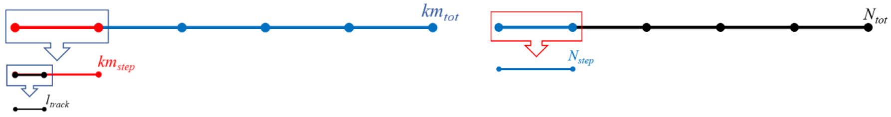
Discretization of the mileage and the total vehicle number.

In this research, an adaptive strategy has been chosen to update the wheel and rail profiles: the approach imposes a threshold value on the maximum of the removed material at each discrete step. Moreover, the update strategy consists of the following steps:

• The removed material on the wheel is proportional to the distance travelled by the vehicle. Thus, the material removed on the wheel has to be scaled according to the following law

$${\mathrm{\Delta }}_j^w\left(s_w\right)\frac{k{m}_{\mathrm{step}}}{l_{\mathrm{track}}}={\mathrm{\Delta }}_j^{\mathrm{wsc}}\left(s_w\right)$$

(7)

• where $k{m}_{\mathrm{step}}$ is calculated in an adaptive way setting a threshold value $D_{\mathrm{step}}^w$ on the maximum of the removed material quantity on the wheel at each discrete step

$$k{m}_{\mathrm{step}}=k{m}_{\mathrm{prove}}*\frac{D_{\mathrm{step}}^w}{\max \left({\mathrm{\Delta }}_j^w\left(s_w\right)\right)}$$

(8)

• where $\max ({\mathrm{\Delta }}_j^w(s_w))$ corresponds to the maximum value of wear depth obtained from the simulation before the scaling operation and $k{m}_{\mathrm{prove}}$ is the mileage travelled by the vehicle during the dynamic simulations.

• Instead, for the rail, the wear is proportional to the total tonnage burden on the track $M_{\mathrm{tot}}$ and thus to the total number of vehicles operating on the line $N_{\mathrm{tot}}$ (see Figure 7). Therefore, if $N_{\mathrm{step}}$ is the number of vehicles running in a discrete step, the quantity of removed material on the rail at each step will be

$${\mathrm{\Delta }}_{l/r}^r\left(s_r\right)*N_{\mathrm{step}}={\mathrm{\Delta }}_{l/r}^{\mathrm{rsc}}\left(s_r\right)$$

(9)

• where $N_{\mathrm{step}}$ is calculated in an adaptive way imposing a threshold value $D_{\mathrm{step}}^r$ on the maximum of the removed material quantity on the rail at each discrete step

$$N_{\mathrm{step}}=\frac{{D^r}_{\mathrm{step}}}{\max \left({\mathrm{\Delta }}_{l/r}^{\mathrm{rsc}}\left(s_r\right)\right)}$$

(10)

The total tonnage burden on the track during the whole simulation is calculated by multiplying the mass of the single vehicle $M_v$ by the total vehicle number

$$M_{\mathrm{tot}}=N_{\mathrm{tot}}*M_v$$

(11)

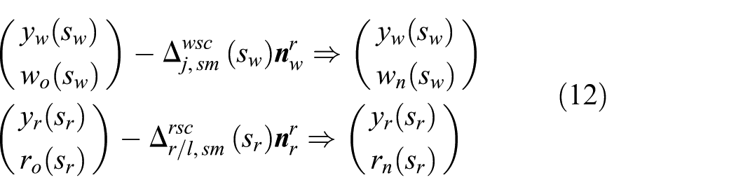
Profile update

Finally, after a smoothing process on the removed material function, necessary to reduce the numerical noise, the new profiles $w_n(s_w)$ and $r_n(s_r)$ are obtained removing the worn material ${\mathrm{\Delta }}_{j,\mathrm{sm}}^{\mathrm{wsc}}(s_w)$ and ${\mathrm{\Delta }}_{r/l,\mathrm{sm}}^{\mathrm{rsc}}(s_r)$ along the normal direction (where the subscript $\mathrm{sm}$ indicates that the profiles have been smoothed, and $n_w^r$ and $n_r^r$ are the outgoing unit vectors for the wheel and rail profile) to the wheel and rail old profile $w_o(s_w)$ and $r_o(s_r)$

$$\begin{array}{c}\left(\begin{array}{c}{y}_w\left(s_w\right)\hfill \\ \multicolumn{1}{c}{w_o\left(s_w\right)}\end{array}\right)-{\mathrm{\Delta }}_{j,\mathrm{sm}}^{\mathrm{wsc}}\left(s_w\right){\mathit{n}}_w^r\Rightarrow \left(\begin{array}{c}{y}_w\left(s_w\right)\hfill \\ \multicolumn{1}{c}{w_n\left(s_w\right)}\end{array}\right)\hfill \\ \left(\begin{array}{c}{y}_r\left(s_r\right)\hfill \\ \multicolumn{1}{c}{r_o\left(s_r\right)}\end{array}\right)-{\mathrm{\Delta }}_{r/l,\mathrm{sm}}^{\mathrm{rsc}}\left(s_r\right){\mathit{n}}_r^r\Rightarrow \left(\begin{array}{c}{y}_r\left(s_r\right)\hfill \\ \multicolumn{1}{c}{r_n\left(s_r\right)}\end{array}\right)\hfill \end{array}$$

(12)

The new updated profiles are then fed back as inputs to the vehicle model, and the whole model architecture can proceed with the next discrete step of the process where a new dynamic simulation and a new profile updating procedure are carried out.

Because of the different scales of magnitude, the wear evolution on wheel and rail has been decoupled (see Figure 8). In particular, since its variation due to wear is negligible in the considered time scale, the rail is supposed to be constant while the wheel wear evolves. On the contrary, each discrete rail profile comes in contact, with the same frequency, with each possible wheel profile. Then, the whole wheel wear evolution (from the original profile to the final one) has been simulated inside each rail step.

Figure 8.

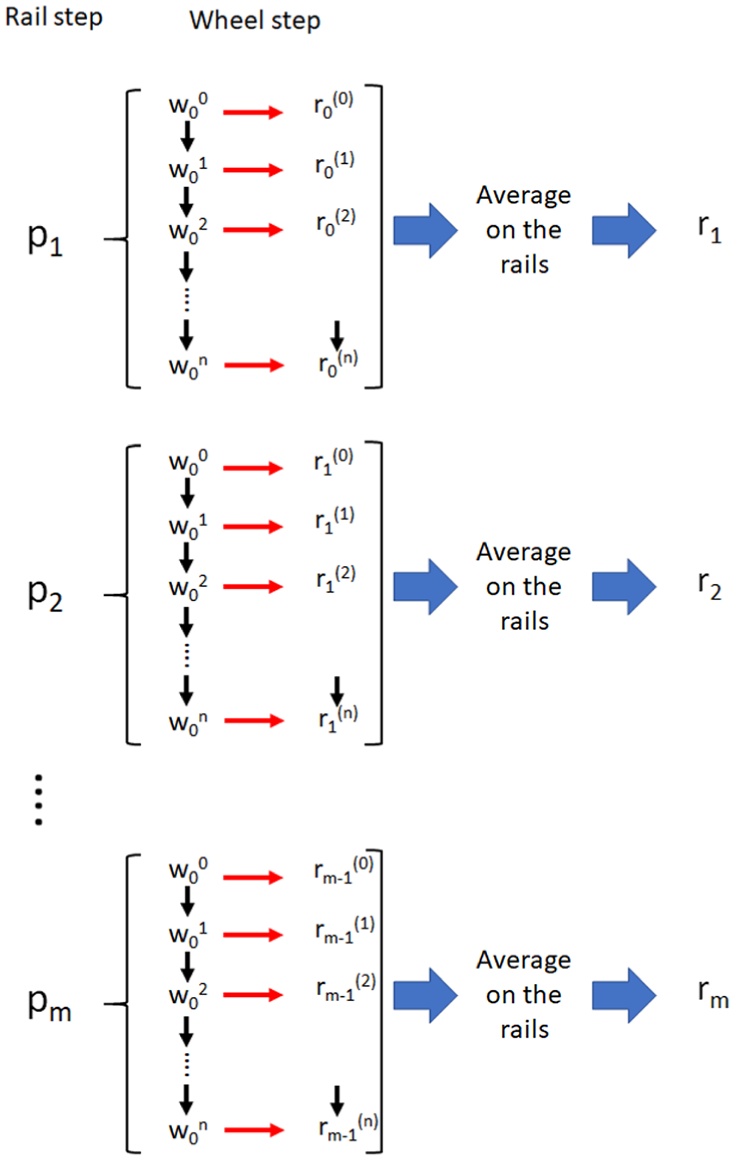
Simulation strategy.

More specifically, in the first discrete rail step p₁, the wheel, starting from the unworn profile $w_0^0$ , evolves on the unworn rail profile r₀ to produce the discrete wheel profiles $w_0^1,w_0^2,...,w_0^n$ . Then, the virtual rail profiles $r_0^0,r_0^1,\cdots$ obtained by running each different wheel profile $w_0^1,w_0^2,...,w_0^n$ on the initial unworn rail profile r₀ are arithmetically averaged to obtain the updated rail profile r₁, used as input in the next discrete rail step. This procedure can be repeated m times in order to perform all the rail steps (see Figure 8).

Measuring instruments and software

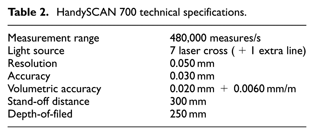
The new measuring instrument used in this work is the optical noncontact 3D laser scanner HandySCAN 700 produced by Creaform Inc (Levis, Quebec) (see Figure 9), suitable for a wide range of industrial applications and engineering services.^25–32 It is completely portable and easy to handle and use but characterized by a very high accuracy and reduced data processing time. Moreover, it allows also the scan of reflecting objects. The main technical specifications are shown in Table 2. The 3D acquisition software VXelements is directly embedded on board and allows the real time 3D reconstructions of any shapes without further additional data editing procedure. The scan is performed by positioning physical targets on the object and/or on the scene, to build a reference positioning model. The following wear mapping and inspection procedure were performed by means of VXmodel and VXinspect, integrated in VXelements software suite. The first one enables 3D scanned data to be used directly in any CAD software, optimizing and cleaning the acquired mesh and applying reverse engineering procedures. The latter allows complete inspection procedures by direct comparison between the scanned part with the nominal CAD project or with the imported mesh of the unworn part to obtain the wear distribution.

Figure 9.

HandySCAN 700.

Table 2.

HandySCAN 700 technical specifications.

Measurement range	480,000 measures/s
Light source	7 laser cross (+1 extra line)
Resolution	0.050 mm
Accuracy	0.030 mm
Volumetric accuracy	0.020 mm + 0.0060 mm/m
Stand-off distance	300 mm
Depth-of-filed	250 mm

Before carrying out the experimental campaign on the real track, to preliminarily test the acquisition procedure, a detailed laboratory analysis has been performed on a straight 500-mm length rail section manually worn out (see Figure 10). First of all, the scanned unworn rail was compared with the reference CAD model to prove the quality of the considered rail section. Then, the scanned worn rail portion was compared with the reference CAD model to evaluate the wear of the surface. Finally, the two unworn and worn scanned rail sections were compared to reproduce the real on-track acquisition procedure.

Figure 10.

Rail section used in laboratory analysis to preliminarily test the acquisition procedure.

Test case and experimental data

The considered test case is the Florence tramway that connects the railway station Santa Maria Novella to the suburban area of Florence (see Figure 2), characterized by very narrow curves (also with radius smaller than 50 m). The line is approximately 7.4 km long, with 14 intermediate stops, and equipped with the standard track gauge (1435 mm). The rail wear evolution has been evaluated on the narrowest curve of the whole network (named A-V08), the most critical in terms of wear, due to its small radius (equal to 25 m). The curve layout is shown in Figure 11. The vehicle runs through the curve at a speed of 14 km/h.

Figure 11.

Curve A-V08 layout.

As said in the introduction, in this phase of the research work, the wear model validation is focused on the rail. The validation has been carried out considering rail experimental data acquired by means of the new accurate 3D optical laser scanner (wear maps). As well, the reference wear parameters acquired by a commonly used 2D measurement instrument have been considered to have a more complete model validation.

3D optical scanning campaign

The measuring campaign with the 3D optical scanner started by placing a set of physical targets close to the rail in order to create a positioning model, made of reference points. After the generation and also optimization of the reference model by software tools to enhance the accuracy, the scanning procedure was performed by HandySCAN 700 generating the 3D model of the rail in real time (Figure 12).

Figure 12.

A 3D optical scanning campaign.

Two measurement campaigns using the optical scanner have been performed on 10 March and 26 September 2016, and the scanned rail surfaces have been used to validate the model in terms of rail shape evolution. During the considered time period, no grinding operations have been done on the track. The results of the acquisitions are saved as mesh files in a stl format and then converted to a step file by means of an ultra-accurate reverse engineering procedure, based on a perfect fitting of parametric surfaces onto the measured mesh. The resulting 3D models of the rails related to the two acquisition campaigns have been cut by using orthogonal planes in the investigated zone of the curve. Subsequently, the unworn and worn 2D rail profiles are obtained from the intersection between the 3D scanned meshes of the rail and such reference planes. For the complete workflow, see Figure 13.

Figure 13.

Workflow to obtain 2D rail profiles starting from 3D surfaces.

By way of example, the difference between the worn (acquired during the second measuring campaign carried out in September) and the unworn reference profile (reference CAD model) of the considered curve is shown in Figure 14. The colour map highlights the different wear depths along the rail.

Figure 14.

Rail 3D wear map.

Furthermore, the large amount and quality of the measured data could be better appreciated considering that the cross sections are taken every 100 mm (see Figure 14). In Figure 15, as an example, four cross sections of the considered curve are shown. From these sections, after a comparison between the nominal rail profile (reference CAD model) with the scanned one, it is possible to evaluate the tread and flange and check the rail conditions to get a clear and complete wear assessment. The red zone in the groove and on the checkrail top (red colour indicates positive wear values) are due, respectively, to the presence of sediments and oxides. The flange wear is higher especially in the central area of the rail where about 9 mm of removed material has been measured with reference to the nominal rail profile (reference CAD model). In the curves characterized by very narrow radius, wear on the checkrail is present as well.

Figure 15.

Cross sections.

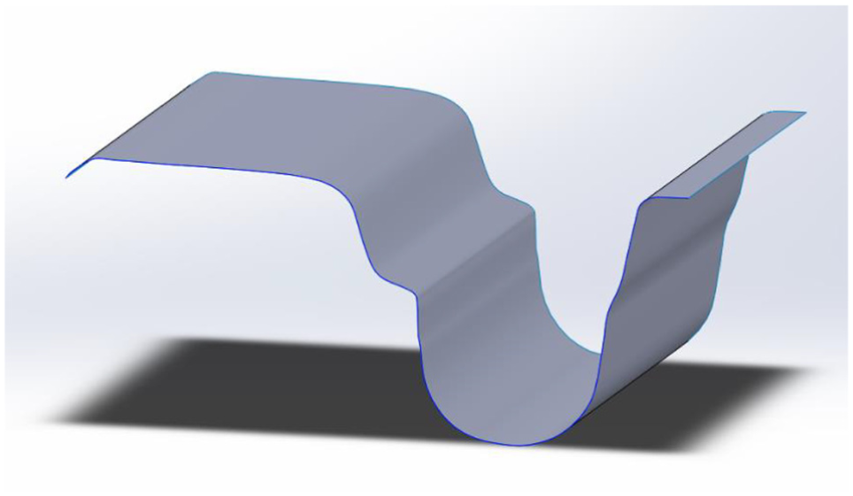
Since the grinding operations in the considered scenario are ‘targeted’ (i.e. the operator locates the spot along the rail where an addition of material is needed, according to the line maintenance plan previsions, he welds on it the new material and then he grinds to re-establish the rail profile), a specific 100-mm long section obtained by means of the procedure previously described and corresponding to the zone highlighted with a red square in Figure 14 has been considered for the wear model validation. The considered rail section is shown in Figure 16 for the first 3D scanner acquisition performed in March 2016 and in Figure 17 for the second one, performed in September 2016. In Figure 16, it is also possible to notice the 2D starting rail profile used in the simulations highlighted in red.

Figure 16.

Considered rail section related to the first measurement campaign.

Figure 17.

Considered rail section related to the second measurement campaign.

To have a clearer wear assessment, in Figure 18, the distribution of wear on the surface of the considered section of rail is shown: in particular, the difference measured in the normal direction between the two on-line scanner acquisitions is reported.

Figure 18.

Surfaces comparison between first and second measurement campaign.

Contact profilometer

The contact profilometer is an electronic hand-pushed trolley able to measure the main wear reference parameters as a function of the travelled distance. In particular, lateral wear has been considered because it directly provides the wear status of the track and by which the maintenance operations are scheduled. Three measurement campaigns have been performed, from March to September. According to the maintenance plan, during this period, no maintenance operations have been done on the considered track section. Processing the measured data, during the considered time period, a lateral wear equal to 2.6 mm on the outer rail has been observed; the related trend is shown in Table 3.

Table 3.

Experimental lateral wear values.

	March 2016	May 2016	September 2016
Lateral wear (mm)	0	1.3	2.6

The model validation will be carried out taking into account both the lateral wear measured through the contact profilometer and the wear measurement acquired by means of the laser scanner (Figure 19).

Figure 19.

Contact profilometer.

Wear model validation

As mentioned in the previous sections, experimental data acquired by means of the optical 3D scanner have been considered for the model validation. In particular, the scanned profiles have been used to validate the model in terms of rail shape evolution. In Figure 20, the comparison between experimental and simulated 2D rail profiles obtained after five rail discrete steps of the wear loop is shown: the continuous red line corresponds to the first scan carried out in March 2016 (see Figure 16) while the black one to the last scan performed in September 2016 (see Figure 17). The blue dashed lines are the simulated rail profiles. The wear is mainly concentrated on the flank zone (see also the zoom in Figure 21), and the simulated results show a good agreement with the real wear evolution.

Figure 20.

Experimental and simulated rail profiles comparison.

Figure 21.

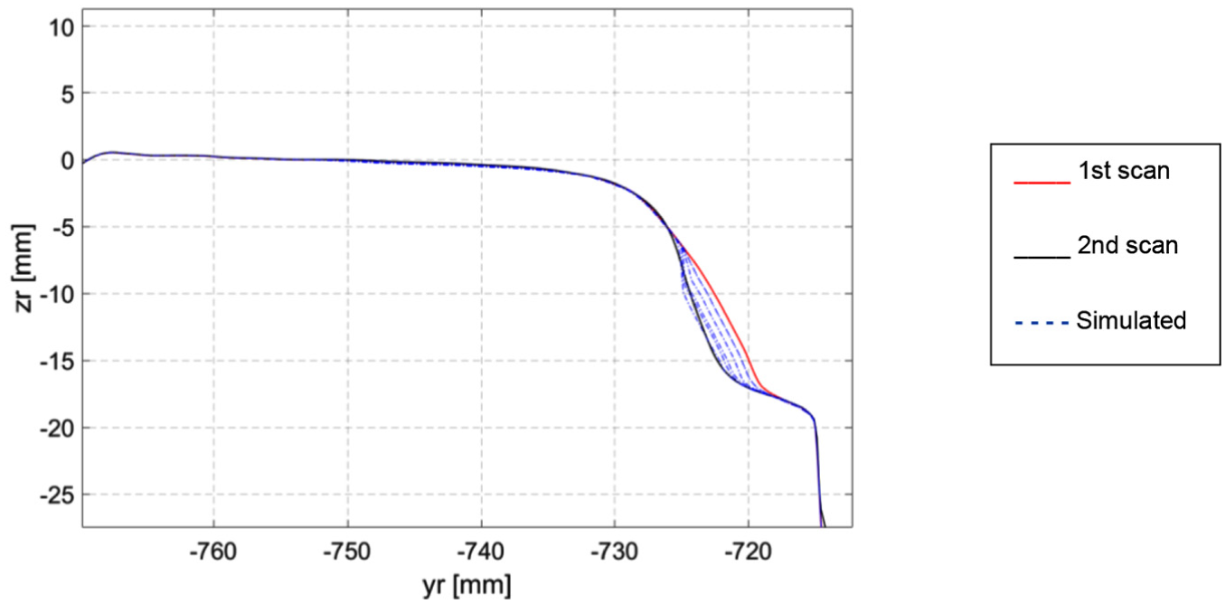
Experimental and simulated rail profiles comparison—zoom on rail flank zone.

In Figure 22, the comparison between the lateral wear values obtained as output of the wear model and those measured through the contact profilometer and the optical 3D scanner is shown. The lateral wear amounts are plotted as a function of the number of vehicles running on the line, calculated considering the real timetable provided by the research partner GEST S.p.A (see Tables 4 and 5). Also, in this case, the results obtained from the wear model can be considered satisfactory.

Figure 22.

Comparison between experimental and simulated lateral wear.

Table 4.

Experimental lateral wear as function of the vehicles number.

Vehicles No.	0	22,088	51,145
Lateral wear (mm)
Contact profilometer	0	1.3	2.6
3D scanner	0	–	2.5

Table 5.

Simulated lateral wear as function of the vehicles number.

Vehicles No.	0	8,880	18,132	27,834	37,829	47,995
Lateralwear (mm)	0	0.5	1.1	1.7	2.3	2.4

Conclusion

This article presents the development and the experimental validation of an efficient wear model able to predict both the wheel and rail shape evolution as a function of the mileage travelled by the vehicle and the number of operating trains, respectively. In this context, the aim of this research work was the experimental validation of the wear model by exploiting a new ultra-accurate laser 3D measurement instrument. In this phase of the work, the focus was set on the rail wear of a reference section of the Florentine tramway line (the narrowest curve of the line and the most critical in terms of wear).

In particular, the data collected by means the 3D laser scanner have been used to study the shape evolution of the rail profile. Moreover, to complete the model validation, the experimental data coming from a classical contact profilometer, the measurement instrument currently adopted for wear inspection on the Florence tramway line, have been considered to investigate the lateral wear.

In both cases, the results obtained from the comparison are satisfactory, highlighting the good accuracy of the model.

It has to be pointed out how the 3D laser scanner allowed a more accurate study of the rail profile evolution than the contact profilometer, providing a clearer and more complete picture of the wear distribution over the whole rail surface. Furthermore, thanks to this innovative measurement method, it becomes easy to detect and study particular 3D wear phenomena as corrugation, plastic flow and so on, not easy to be analyzed even through the most accurate 2D measurement instruments like 2D laser profilometers.

As a future development, further measurement campaigns using 3D laser scanners are already scheduled on other critical curves of the Florence tramway line to better evaluate the accuracy of the model. At the same time, the model validation via 3D laser scanners will be also extended to wheel wear despite the greater difficulty in performing the measurements. Moreover, an innovative 3D wear model will be implemented, especially concerning the rail wear, to obtain as output a spatial distribution of the wear on the rail surface. This way, 3D wear phenomena such as corrugation and plastic flow will be better investigated and the related 3D model will be better validated, thanks to the employment of new 3D optical scanners. Furthermore, the authors are working to include into the wear model the thermal effects and the hardening of the materials to have an even more accurate wear assessment. Finally, the authors are performing new experimental tests directly on field and on test rigs to calibrate the wear law under more general and realistic conditions (including wet contact and contaminants and different environmental temperatures) to get a more accurate wear estimation.