Sage Journals: Discover world-class research

Abstract

This article presents a vibration-based technique for damage detection in the cylindrical equipment. First, a damage index based on the residual frequency responses is defined. This technique uses the principal component analysis for data reduction by eliminating the components that have the minimum contribution to the damage index. Then, the principal components are fed into neural networks to identify the changes in the damage pattern. Furthermore, the efficiency of this technique in the field condition is investigated by adding different noise levels to the output data. This study aims at proposing a cost-effective damage detection model using only one sensor. Therefore, the optimal location of the sensor is also discussed. A case study of capacitive voltage transformer is used for validation of finite element models. The neural networks are trained using numerical data and tested with experimental one. Several parametric analyses are performed to investigate the sensitivity of the model.

Keywords

Cylindrical equipment neural networks experimental test sensor noise optimal location

Introduction

This article presents a vibration-based technique for damage detection in the cylindrical equipment (e.g. capacitive voltage transformer (CVT) equipment). The power transmission substations are susceptible to damage under seismic excitations.¹ Figure 1 shows some of the damaged equipment in Bam substation, Iran, during the 2003 devastative Bam Earthquake.

Figure 1.

Failure in electrical equipment during the Bam earthquake: (a) porcelain parts and (b) leakage in capacitive transformer.²

Since the repair and replacing cost of those damaged equipment is considerable, it is important to quantify the damage level a priori and take the required actions with respect to the damage severity. The process of detecting and tracking the structural damage is known as the structural health monitoring (SHM).^3,4 The presence of a damage in a structural system alters its physical properties, which subsequently affects the dynamic properties such as natural frequencies, mode shapes, and modal damping. Therefore, the damage state of a structure can be identified through examining its dynamic parameters.⁵ Generally, the dynamic properties of a structure can be determined by evaluating its time history responses, frequency response functions, and modal parameters.⁶

Pattern recognition is a promising method for discovering the structural damages.⁷ The basic idea of the damage recognition based on a neural network (NN) relies on defining the damage index (DI) of the model as an input for the NN, while the corresponding damage scenario is defined as the target. The NN, trained by fitting the features measured on the network inputs, has the ability to estimate the damage conditions in the structure.⁸

Many researchers have tried to identify the failures in different structures using NN capabilities. Gonzalez-Perez and Valdes-Gonzalez⁹ used an NN model to identify the damages in vehicular bridges. They used the modal strain energy to train the networks. Elshafey et al.¹⁰ used the NN and random decrement technique to obtain the free vibration of the system and examined the damage in the laboratory model of a offshore structure. Tan et al.¹¹ investigated the damage in simply supported beams using an NN-based technique combined with a modal strain energy-induced DI as an input to the network. Zang et al.¹² proposed a simple method based on the structural response in time domain and NN to detect the damage. Due to the large amount of data in time domain as well as the noise effects, they employed the independent component analysis (ICA). Massari et al.¹³ investigated a method based on the template matching to detect and locate the damage in buildings following severe earthquake shaking. Pakrashi et al.¹⁴ studied a statistical approach on the detection of the presence, the location, and the extent of an open crack from the first fundamental mode shape of a simply supported beam. Sazonov and Klinkhachorn¹⁵ investigated the analytical and numerical arguments to select the optimal mode shape sampling interval to maximize sensitivity of damage detection and the accuracy of damage localization. In a very comprehensive research, Ghiasi et al.¹⁶ compared several artificial intelligence techniques in damage detection of truss structures including NN, support vector machines, adaptive neural-fuzzy inference system, nearest neighbors, and extreme learning machine.

Application of the damage detection techniques in vulnerability assessment of the equipment in electrical industry is very limited. Yin et al.¹⁷ performed damage detection of a transmission tower using ambient vibration test. They adopted a method to identify the structural mode shapes along with dynamic reduction technique to detect the damage location. Lam and Yin¹⁸ verified the method employed by Yin et al.¹⁷ through experimental tests and applied it to a 2.4-m-high tower. They also investigated the sensor placement and computational efficiency.

In the light of the previous studies, this article proposes a method based on NN for damage detection in cylindrical equipment. The method relies on principal component analysis (PCA) to reduce the data size and employs NN to detect the damage patterns. To examine the accuracy of the proposed method, different damage scenarios are studied. Moreover, to evaluate the performance of the method under the field condition, a white Gaussian noise with different intensities is added to the structural response. In addition, this study aims at detecting the structural damage in a very cost-effective method by using only one sensor. Therefore, the optimal location of the sensor plays an important role on the accuracy of the results. Last but not least, the method is applied to a small-scale experimental model to evaluate its efficiency in detection of the damage location and its severity. This technique can be extended to the similar equipment and even nonstructural components.

Review of theoretical background

This section provides a very short review on the principals of the PCA and NN for the readers with these techniques. It provides a smooth transition from theoretical formulations to the numerical and experimental models.

PCA

PCA, developed by Jolliffe and Cadima¹⁹ and Bishop,²⁰ is a technique that compresses the data linearly and is widely used in image processing, flow visualization, pattern recognition, and time-series prediction fields. In fact, the process of extracting eigenvalues of the covariance matrix of the data is the basis of this technique. PCA is a statistical technique, which performs a dimension reduction on the variables space. Using this analysis, the original set of variables in an N-dimensional space is transformed into a new set of uncorrelated variables in a P-dimensional space where P < N.²¹

The following presents the procedure by which the principal component for $x_{ij}$ dataset is derived. First, the mean value of the jth column, $μ_{j}$ , and the corresponding standard deviation, $σ_{j}$ , are computed. Then, each element of the dataset is normalized, ${\tilde{x}}_{ij} = (x_{ij} - μ_{j}) / σ_{j}$ . The covariance matrix is defined as $[cov] = [\tilde{x}]^{T} [\tilde{x}] / n - 1$ , where $n$ is the number of measurements. Finally, the principal components are simply obtained by solving the eigenvalue problem: $[cov] {E_{i}} = λ_{i} {E_{i}}$ , where $λ_{i}$ is the ith eigenvalue and $E_{i}$ is the corresponding eigenvector.

The first principal component that has the highest eigenvalue and the eigenvector associated with it indicates the direction and the amount of maximum variability in the original data. The second principal component, which is orthogonal to the first component, indicates the next most significant contribution to the original data and so on. By eliminating the components with least contributions to the dataset, the data size can be reduced effectively.²¹ The projection of the response matrix on the $r$ principal components is given as follows

{[A]}_{n \times r} = {[X]}_{n \times r} {[E]}_{n \times r}

(1)

The projection matrix, $A$ , and the eigenvectors matrix, $λ$ , can be divided into (1) $p$ principal components that have the highest contributions to the dataset and (2) the remaining $r - p$ least important principal components. The choice of $p$ is critical to successful data compression. The value of $p$ is determined by considering the contribution rate of each component, and the effect of noise on components is determined accordingly.

By eliminating $r - p$ components, the reduced data matrix is obtained as follows

\begin{matrix} {[{\tilde{X}}_{R}]}_{n \times r} = [{[A]}_{1 \times p} : {[0]}_{1 \times (r - p)}] \\ {[{[E]}_{r \times p} : {[0]}_{r \times (r - p)}]}^{T} \approx {[A]}_{n \times p} {[E]}_{p \times r}^{T} \end{matrix}

(2)

PCA is a powerful method to reduce the effects of measurements noise on data. Since the measurements noise has a random nature, there is no clear correlation between noise and data. Therefore, deleting the components with less contribution acts like a filter and reduces the effect of noise on data.¹⁹

NN

NN is a powerful tool for pattern recognition and data classification. The architecture of an NN comprises four elements: (1) the number of layers (the neurons are organized in groups called layers), (2) the number of neurons in each layer, (3) the activation functions of each layer, and (4) the training algorithm. The layers are subsequently divided into output layers and hidden layers. The output layers are associated with the NN output, while the other layers are categorized as the hidden layers.²²

The number of neurons can vary between different layers, and each neuron is an independent element. The training algorithm is selected based on the bias and final weight values of the NNs.²³ The most commonly used networks for damage detection are multi-layer NNs coupled with the backpropagation algorithm.²⁴ The output of a feed-forward network with $s$ hidden layers is given as follows

a_{k} (p) = \sum_{j = 1}^{s} (w_{kj} f (\sum_{i = 1}^{d} w_{ji} p_{i} + b_{j 0})) + b_{k 0}

(3)

where $p_{i}$ is the input, $b_{j 0}$ and $b_{k 0}$ are the bias parameters, $w_{kj}$ and $w_{ji}$ are the inter-connection weights, $d$ is the number of input units, and $f$ refers to the transfer function. Note that each layer can have a different transfer function. In this research, a nonlinear sigmoidal transfer function is adopted for all the layers in the form of

f (x) = (1 + e^{- x})^{- 1}

(4)

The NN is trained to minimize errors on the training dataset and also to maximize its accuracy when new inputs are introduced to the network. For this purpose, the “Bayesian regularization” algorithm is used in which the weight and bias values are updated according to Levenberg–Marquardt optimization technique. It minimizes a combination of squared errors and weights and then determines the correct combination to establish a generalized network.^25,26

Methodology

In this research, a vibration-based method is proposed for damage detection in CVTs. Methods based on frequency response functions have been investigated in the previous studies. In this research, a DI based on residual frequency response of the structure under impact excitation is defined. The residual frequency response is the difference between the intact and the damaged structure.

This method is first implemented on a numerical model. Then, the improved version is applied in the field condition. The designed NN for the numerical simulation is utilized for damage detection (both the location and severity) of field dataset. Figure 2 illustrates the proposed damage detection algorithm.

Figure 2.

Damage detection algorithm.

Algorithm implementation

Numerical model

The first numerical model is a CVT developed in SAP2000 program. The configuration of the system is shown in Figure 3 as provided by the manufacturer. In this model, the porcelain insulator, cement material, and aluminum flanges are considered as eight-noded solid elements with a maximum dimension of 0.02 m. Moreover, the oil tank is modeled using four-noded shell elements with a maximum dimension of 0.05 m.

Figure 3.

Capacitive voltage transformer system: (a) elements and (b) support structure.²

The material properties of each part are summarized in Table 1. The supporting structure consists of the steel elements: the vertical members of the supporting structure are in $L 60 \times 60 \times 6$ angles and the diagonal members are in $L 40 \times 40 \times 4$ angles. These properties are based on the IEEE Standard-693 recommendations. According to the IEEE recommendations, the damping ratio of this equipment is assumed to be 2%. In order to account for the oil mass inside the tank, as well as the porcelain insulator, additional masses are symmetrically added to the insulator and the tank walls.

Table 1.

Material properties of each element in CVT; $γ$ : specific weight and $E$ : modulus of elasticity.

Name	Element type	Properties	$γ$ (kgf cm)	$E$ (kgf cm)
Leg	Elastic	Steel	7.85E−03	2.10E+06
Oil tank	Shell	Aluminum	7.50E−03	7.04E+05
Flange	Shell	Aluminum	2.70E−03	7.04E+05
Cement	Shell	Special cement	7.85E−03	2.50E+05
Porcelain	Solid	Porcelain	5.48E−03	7.10E+05

CVT: capacitive voltage transformer.

The height and total mass of the porcelain insulator and bottom flange are 2.4 m and 330 kg, respectively. The similar parameters for the oil tank are 0.6 m and 200 kg, respectively. The total stiffness of the CVT is 2.81 MN/m². The natural frequency of the CVT (without equipment support) is 8.95 and 8.90 Hz according to the equipment catalog and the finite element model, respectively. Traditionally, the numerical model is verified by comparing its frequency response with experimental one. In the current example, the first mode is captured with only 0.6% error. One may note that for cantilever-type structures, the first model is the dominant one.

Damage scenarios and loading details

To examine the effectiveness of the proposed method, different damage scenarios are considered as shown in Figure 4. According to this plot, three damage severities (denoted as D15%, D30%, and D50%) including 15%, 30%, and 50% element removal from the insulator are considered. The width of the cracks is assumed to be 0.005 m in all cases. Moreover, 18 damage locations (shown as L01 to L18) are taken into account along the height, with the distance of 0.12 m from each other. Finally, four damage angles (shown as a1 to a4) are modeled along the perimeter. 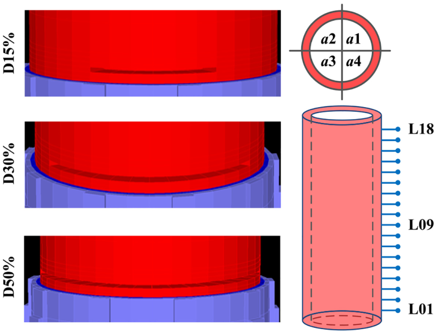Therefore, a combination of $3 \times 18 \times 4 = 216$ dataset is generated to train the NN. Again, the goal is to detect the location and severity of the cracks occurred along the porcelain insulator.

Figure 4.

Illustration of the damage severity, location, and angle.

In this section, only one sensor (located at the top of the bottom aluminum flange) is used to record the responses under the impact excitation. The ramp-type impact load is applied at point A of structure as shown in Figure 5, with the angle of 45° with respect to both axes.

Figure 5.

Illustration of the impact location, angle, recording directions, and loading details.

For each of the 216 damage scenario, there are two frequency responses with the total duration of 2.0 s recorded at 0.001 s time step in the horizontal and vertical directions. For each damage scenario, the frequency response of the damaged structure is subtracted from the one resulted from sound structure and is called the residual frequency response. Overall, 216 averaged residual frequency responses are collected. Therefore, a matrix of data with the size of $216 \times 300$ is formed, in which 216 refers to the number of samples and 300 presents the sample size. Figure 6(a) shows the effect of damage on the frequency response of the structure, while the impact of different damage locations on the residual responses is shown in Figure 6(b). As seen, the location of peak residual responses corresponds to the peak frequency responses in healthy and damaged structures.

Figure 6.

Effects of light damage on vibration response: (a) frequency response at L12 and (b) residual responses at different locations.

The PCA is performed on the data matrix and the number of components used to train the NN is determined based on the contribution of each component and the effect of noise on them. The remaining components are used as the DI instead of the residual frequency response to train the NNs.

According to Figure 7, it is clear that different damage scenarios have different principal component patterns. In general, lower locations provide higher quantity for the principal components. Furthermore, a more severe damage scenario leads to higher variation in the principal component.

Figure 7.

Variation of the first 10 principal components for different damage scenarios: (a) impact of location; all small damage and (b) impact of severity; all L09 damage.

To detect the damage location and severity, NNs are employed. The principal components of each damage scenario are fed to the NN as DI. A sensitivity analysis is performed to determine the minimum number of the layers, as well as the number of the neurons in each layer. The architecture of the NN can be summarized as follows:

Bayesian regularization is used as training algorithm.

Sigmoid transfer function is used for all the layers.

There are three layers in the models.

A total of 10 principal components are used in each case.

There are 14 and 3 neurons in first layer if the target is damage location and damage severity, respectively.

There are 6 and 3 neurons in second layer if the target is damage location and damage severity, respectively.

It should be noted that the simple hold-out technique is used to generalize the trained networks.

The networks are fed with the principal components of each damage scenario and are trained to detect the damage location and severity by determining the target function and trying different sets of network parameters. The normalized error, $Er r_{norm}$ , criterion is used to evaluate the performance of the trained networks. This criterion is expressed as follows

E r r_{n o r m}^{β} = \frac{\sum_{i = 1}^{n} \frac{{| NO - NT |}_{i}}{β_{m a x}}}{n} \times 100 %

(5)

where $NO$ and $NT$ refer to the network output and target, respectively; $β_{\max}$ might take one of the following forms depending on whether it is used for location or severity damage detection: $L_{\max}$ (length of the insulator) or $D_{\max}$ (maximum severity); and finally, $n$ is the size of the data.

During the training process, for each scenario, 10 networks are used to reduce the uncertainties associated with damage detection. The average normalized error is 0.182% and 0.021% for the location and severity detection, respectively. To evaluate the performance of the trained NNs, four new damage scenarios are defined, which were not included in the training step, and the results of the damage detection are reported in Table 2. In the first three scenarios, the objective is to predict the unknown damage location with a fixed damage severity value (i.e. 15%). One should note that 15% is the lower bound for damage severity training (i.e. (15%, 50%)) and thus is considered as a worst-case scenario. It is expected that the performance of the system will get better for higher damage severity percentages. As seen, the error of predicted damage severity is zero, and those from unknown locations are pretty negligible.

Table 2.

Evaluation of trained neural networks.

Scenario	Target	NT	NO	$Er r_{norm}$
1	Location	18 cm	18.71 cm	0.32%
	Severity	15%	15%	0
2	Location	90 cm	90.18 cm	0.08%
	Severity	15%	15%	0
3	Location	150 cm	151.32 cm	0.60%
	Severity	15%	15%	0
4	Location	114 cm	110.22 cm	1.80%
	Severity	25%	22%	3%

NO: network output; NT: network target.

Scenario 4 is based on 10% noise.

In scenario 4, both the damage location and its severity are assumed to be unknown simultaneously. The target location and severity are set to 114 cm (which is between 108 and 120 cm points) and 25% (which is between 15% and 30% damage), respectively. For this combined scenario, the developed NN predicts the location and severity with 1.8% and 3.0% errors, respectively (see Table 2).

Noise effect

To account for the field condition, a white Gaussian noise is added to the structural responses. Three noise-to-signal ratios of 2%, 5%, and 10% are generated to evaluate the model sensitivity. The noise has a random nature and affects all the components including those with less significance. Therefore, by eliminating the low contribution components, the effect of noise on the accuracy of the results is decreased. To determine the number of principal components which are not affected by the noise (for each noise level), the noise is iteratively added to the responses multiple times and the PCA is performed for each case. The components which demonstrate the highest variations are eliminated from the computations. This operation is shown in Figure 8 for a scenario in which the damage occurs on L09.

Figure 8.

Uncertainty in principal components with different noise ratios; results are at L09: (a) without noise, (b) 2% noise, (c) 5% noise, and (d) 10% noise.

Figure 8(a) presents the case where no noise is introduced to the model. As a result, this is a deterministic curve for the idealized condition. Figure 8(b) presents the first 10 components of the structure with 2% noise. Since the noise does not practically have any effect on the first 10 components, all of them are used to train the NNs. According to Figure 8(c), the first five components are not affected in the case of adding 5% noise to the system. Thus, only the first five components are selected in the training process, and the others are eliminated. Finally, the impact of 10% noise is shown in Figure 8(d), and only the first four components are used for NN training. It is noteworthy that to evaluate the trained NNs, three damage scenarios are assumed and the results are reported in Table 3. The goodness of fit for both the train and test data is shown in Figure 9 for the model with 10% noise (worst-case scenario).

Table 3.

Evaluation of trained neural networks including noise effects.

Noise	Scenario	Target	NT	NO	$Er r_{norm}$
2%	1	Location	18 cm	18.97 cm	0.44%
		Severity	15%	15%	0
	2	Location	90 cm	91.05 cm	0.47%
		Severity	15%	15%	0
	3	Location	150 cm	149.05 cm	0.43%
		Severity	15%	15%	0
5%	1	Location	18 cm	19.10 cm	0.50%
		Severity	15%	15%	0
	2	Location	90 cm	91.25 cm	0.57%
		Severity	15%	15%	0
	3	Location	150 cm	148.58 cm	0.65%
		Severity	15%	15%	0
10%	1	Location	18 cm	24.12 cm	2.78%
		Severity	15%	15%	0
	2	Location	90 cm	96.32 cm	2.87%
		Severity	15%	15%	0
	3	Location	150 cm	159.32 cm	4.32%
		Severity	15%	15%	0

Figure 9.

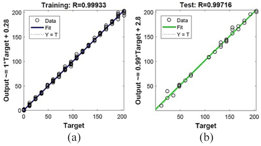
NN-based goodness of fit for train and test data; the case with 10% noise.

Optimal sensor location

Since only one sensor is used to detect the location and the severity of the damage, it is necessary to determine an optimal location which yields the least error. For this purpose, five different locations along the height of insulator are selected with a uniform distance of 50 cm. They roughly corresponded to L01, L05, L09, L13 (of L14), and L18 in Figure 4.

For each damage scenario, and each noise level, the normalized error of the training data is calculated, and the location with the minimum $Er r_{norm}$ is selected as an optimal place for the sensor. For each sensor location and each noise level, 10 networks are trained and the sum of the $Er r_{norm}$ from all the networks is used as an index to evaluate the optimality of the location. The $Er r_{norm}$ for each sensor location and each noise level is shown in Figure 10. Obviously, higher noise increases the normalized error. Shown in this plot is also the mean value of different noise levels for each location. Overall, L05 seems to be the optimal location for sensor location.

Figure 10.

Optimal sensor location considering noise effect.

Experimental test setup

The proposed method in the previous sections is examined through an experimental program. For this purpose, a similar structure to the numerical model of CVT is built by the authors (Figure 11(a)). The structure is made up of an U-PVC pipe which is connected to a rigid base with four bolts, a steel pipe, and a steel sheet. The space between the U-PVC pipe and the steel pipe is filled with cement. Diameter and thickness of the U-PVC pipe are 0.125 m and 0.0032 m, respectively. The height of the U-PVC pipe is 1.31 m.

Figure 11.

CVT models: (a) experimental, (b) FE, and (c) three damage scenarios.

Model updating technique is used to obtain modulus of elasticity of the U-PVC pipe. For this purpose, the numerical model of this structure is established in SAP2000 (Figure 11(b)). The body of the U-PVC pipe is modeled with shell elements. The natural frequency of the first mode of the structure is considered as the target parameter in the model updating process. Using this method, the modulus of elasticity of the U-PVC pipe is obtained as 496,200 kg/cm². Since the connection to the base is not completely rigid, some translational and rotational springs are used in the numerical model to connect the structure to the base. In addition, using the aforementioned method to model the base connection improves the accuracy of the numerical model in higher modes of vibration. Natural frequencies of the numerical and the experimental models are compared in Table 4.

Table 4.

Comparison of the natural frequencies of experimental and numerical models.

Mode	Numerical (Hz)	Experimental (Hz)	Error (%)
1	25.49	25.49 Hz	0.00
2	134.10	134.01 Hz	0.06
3	196.80	198.17 Hz	0.69
4	241.10	240.41 Hz	0.29

In this study, the structure is excited with a pendulum thrown from a specified height. It hits the structure at a distance of 0.1 m from the bottom of the U-PVC pipe. A series of “Kyowa AS-5GB” sensors are used to record the response of the structure. These sensors are installed at a distance of 0.15 m from the top of the U-PVC pipe. The recording sample rate is considered 1000 Hz. The NN training is performed with 23 damage locations along the U-PVC pipe uniformly distributed at 0.05 m distance from each other. In each damage location, three damage severities including small, medium, and high are implemented.

In the case of small damage, the elements of the structure with 0.022 m length and 0.0025 m width are removed. In damage with medium severity, the elements with 0.044 cm length and 0.0025 m width are removed, and finally for severe damage, the elements with 0.066 m length and 0.0025 m width are removed. Note that each damage scenario is considered to occur in four angles around the structure. Therefore, the total number of NN inputs is $4 \times 3 \times 23 = 276$ . It should be noted that the NNs are trained with numerical models and tested with experimental data. To evaluate the performance of the trained NN, three damage scenarios are assumed. A damage with the length of 0.022, 0.044, and 0.066 and 0.0025 m width is formed at a distance of 0.27 m from the bottom of the U-PVC pipe (Figure 11(c)).

In this study, a three-layer feed-forward NN with six neurons in its first and second hidden layers is used. The transfer function of all the layers is set to “tansig.” To take into account the uncertainties associated with the NN training, a number of 50 sample networks are considered for each damage scenario. The results of the damage detection in the first, second, and third scenarios are shown in Figure 12.

Figure 12.

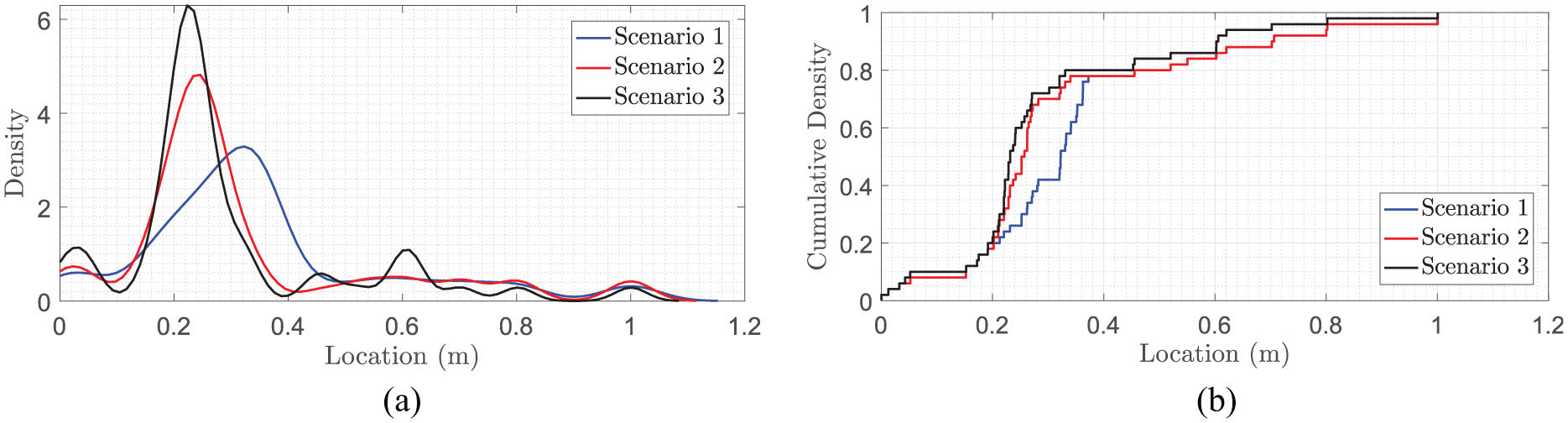
Damage detection in experimental program: (a) Kernel distribution model and (b) empirical cumulative density function.

Figure 12(a) presents the kernel distribution of three scenarios. This is a nonparametric representation of the probability density function of a random variable²⁷ and is used when a parametric distribution cannot properly describe the data or to avoid making assumptions about the distribution of the data. Scenarios 2 and 3 have a close peak (i.e. 0.249 and 0.229 m distance from the bottom of the PVC pipe, respectively), while scenario 1 has its peak at about 0.309 m. In addition, the empirical cumulative density function is shown in Figure 12(b). Again, scenarios 2 and 3 are close, while scenario 1 has a gap between the range of (0.2, 0.4) m. Finally, regardless of the damage severity, its location is detected with a good accuracy.

Conclusion

In this article, a vibration-based method to detect the damage location and its severity in CVTs is presented. The method uses the PCA on residual frequency response functions of the structure under impact excitation and employs NNs to find damage patterns. To examine the effectiveness of the proposed method under field condition, the white Gaussian noise with different scattering is added to the structural response. Based on the analysis results, the method provides fairly accurate results under various conditions.

Furthermore, the accuracy of the damage detection highly depends on the sensor location. Therefore, a part of this study is dedicated to determine the optimal sensor location. This provides a cost-effective method to be used in real-world problems of experimental damage detection. Finally, the presented method is examined through an experiment program, and it is shown that the proposed method is effective in damage detection of the pipe-type structure. In general, both the location and severity can be estimated though this technique.

Footnotes

Handling Editor: James Baldwin

Declaration of conflicting interests

The author(s) declared no potential conflicts of interest with respect to the research, authorship, and/or publication of this article.

Funding

The author(s) received no financial support for the research, authorship, and/or publication of this article.

ORCID iDs

M Mirtaheri

MA Hariri-Ardebili

References

Kwasinski

Eidinger

Tang

et al . Performance of electric power systems in the 2010–2011 Christchurch, New Zealand, earthquake sequence. Earthq Spectra 2014; 30: 205–230.

Mohammadi

Akrami

Nikfar

Dynamic properties of substation support structures. J Construct Steel Res 2012; 78: 173–182.

Al-Khalidy

Noori

Hou

et al . Health monitoring systems of linear structures using wavelet analysis. In: Proceedings of the structural health monitoring–current status and perspectives, proceedings of the international workshop on structural health monitoring, Stanford, CA, 18–20 September 1997, pp.164–175. New York: ASME.

Chang

Flatau

Liu

SC.

Health monitoring of civil infrastructure. Struct Health Monit 2003; 2: 257–267.

Hou

Noori

St Amand

Wavelet-based approach for structural damage detection. J Eng Mech 2000; 126: 677–683.

Mohan

Maiti

Maity

Structural damage assessment using FRF employing particle swarm optimization. Appl Math Comput 2013; 219: 10387–10400.

Moradi

Amin Hariri-Ardebili

Developing a library of shear walls database and the neural network based predictive meta-model. Appl Sci 2019; 9: 2562.

Lam

CT.

The selection of pattern features for structural damage detection using an extended Bayesian ANN algorithm. Eng Struct 2008; 30: 2762–2770.

Gonzalez-Perez

Valdes-Gonzalez

Identification of structural damage in a vehicular bridge using artificial neural networks. Struct Health Monit 2011; 10: 33–48.

10.

Elshafey

Haddara

Marzouk

Damage detection in offshore structures using neural networks. Marine Struct 2010; 23: 131–145.

11.

Tan

Thambiratnam

Chan

THT

et al . Detecting damage in steel beams using modal strain energy based damage index and artificial neural network. Eng Fail Anal 2017; 79: 253–262.

12.

Zang

Friswell

Imregun

Structural damage detection using independent component analysis. Struct Health Monit 2004; 69–83.

13.

Massari

Clayton

Kohler

Damage detection by template matching of scattered waves. Bull Seismol Soc Am 2018; 108: 2556–2564.

14.

Pakrashi

Basu

O’Connor

A statistical measure for wavelet based singularity detection. J Vib Acoust 2009; 131: 041015.

15.

Sazonov

Klinkhachorn

Optimal spatial sampling interval for damage detection by curvature or strain energy mode shapes. J Sound Vib 2005; 285: 783–801.

16.

Ghiasi

Ghasemi

Noori

Comparative studies of metamodeling and AI-based techniques in damage detection of structures. Adv Eng Soft 2018; 125: 101–112.

17.

Yin

Lam

Chow

et al . Dynamic reduction-based structural damage detection of transmission tower utilizing ambient vibration data. Eng Struct 2009; 31: 2009–2019.

18.

Lam

Yin

Dynamic reduction-based structural damage detection of transmission towers: practical issues and experimental verification. Eng Struct 2011; 33: 1459–1478.

19.

Jolliffe

Cadima

Principal component analysis: a review and recent developments. Philos T R Soc A: Math Phys Eng Sci 2016; 374: 20150202.

20.

Bishop

CM.

Neural networks for pattern recognition. Oxford: Oxford University Press, 1995.

21.

Tharwat

Principal component analysis: a tutorial. Int J Appl Pattern Recogn 2016; 3: 197–240.

22.

Daniel

Principles of artificial neural networks, vol. 7. River Edge, NJ: World Scientific, 2013.

23.

Ghiasi

Torkzadeh

Noori

Structural damage detection using artificial neural networks and least square support vector machine with particle swarm harmony search algorithm. Int J Sustain Mater Struct Syst 2014; 1: 303–320.

24.

Haykin

SS.

Neural networks and learning machines, vol. 3. Upper Saddle River, NJ: Pearson, 2009.

25.

Aggarwal

Singh

Pravin

et al . Bayesian regularization in a neural network model to estimate lines of code using function points. J Comput Sci 2005; 1: 505–509.

26.

Dan Foresee

Hagan

. Gauss-Newton approximation to Bayesian learning. In: Proceedings of international conference on neural networks (ICNN’97), vol. 3, Houston, TX, 12 June 1997, pp.1930–1935. New York: IEEE.

27.

MATLAB version 9.1 (R2016b). Natick, MA: The MathWorks Inc., 2016.

A cost-effective neural network–based damage detection procedure for cylindrical equipment

Abstract

Keywords

Introduction

Review of theoretical background

PCA

NN

Methodology

Algorithm implementation

Numerical model

Damage scenarios and loading details

Noise effect

Optimal sensor location

Experimental test setup

Conclusion

Footnotes

Declaration of conflicting interests

Funding

ORCID iDs

References