Sage Journals: Discover world-class research

Abstract

A pantograph in contact with a catenary for power supply is one of the major aerodynamic noise sources in high-speed trains. To reduce pantograph noise, it is essential to understand the noise generation mechanism of the pantograph. However, it is difficult to determine this mechanism through measurement. Therefore, in this study, the aerodynamic and acoustic performances of a pantograph in a high-speed train were investigated through numerical analysis using the lattice Boltzmann method. First, a real-scaled pantograph was modeled through computer-aided design. Then, the surface and volume meshes of the pantograph model were generated for simulation analysis. Numerical simulation was conducted at a speed of 300 km/h based on the lattice Boltzmann method. Based on the time derivative analysis of flow pressures, it was concluded that the panhead, joint, and base were the dominant noise sources in the pantograph. In particular, various vortexes were generated from the metalized carbon strip of the panhead. The peaks of the sound pressure level propagated from the panhead were 242, 430, and 640 Hz. The noise generation mechanism was analyzed through numerical simulation using noise characteristics.

Keywords

High-speed train pantograph aeroacoustics numerical analysis lattice Boltzmann method

Introduction

The aerodynamic noise of high-speed trains increases sharply at a running speed of over approximately 300 km/h.¹ The primary sources of aerodynamic noise are the front nose, pantograph, inter-coach spacing, and so on.^2,3 Among these, the pantograph is composed of protruding shapes in contact with a catenary for power supply.⁴ Therefore, high air resistance and complex flow of the pantograph are inevitable at high speeds. Moreover, it is difficult to measure the propagation noise of the pantograph using microphones because of a high voltage of over 2.5 kV from the catenary. In this regard, studies have been conducted to measure and analyze the aerodynamic noise from the pantograph.

The beamforming method was used to measure and analyze the propagation noise of the pantograph using microphone array systems.^5,6 A microphone array system has the advantage that it can derive noise at specific locations such as bogies or pantographs. However, it is difficult to obtain the aerodynamic noise generation mechanism through measurements performed using microphone arrays. Conducting numerical analysis by employing computational approaches is useful for deriving the noise generation mechanism of the pantograph.

In recent years, two-stage hybrid methods based on computational fluid dynamics (CFD) and computational acoustics have been developed for investigating the noise generation mechanism in high-speed trains.⁷ The aerodynamic and aeroacoustic behavior of the flow past a simplified high-speed train bogie at scale of 1:10 was studied at a flow speed of 30 m/s.⁸ In particular, near-field unsteady flow was obtained by numerically solving the Navier–Stokes equations using the delayed-eddy model, and the results were used to predict far-field noise using the Ffowcs Williams–Hawkings method. A dipole shape was observed for the noise radiated from the bogie, and the noise contribution from the bogie frame was relatively weak compared to that from the wheelsets of the bogie.

However, while hybrid simulation might be able to capture the global characteristics of a small-scaled system in a few cases, it does not allow for the prediction of the actual highly unsteady flow field present in the system during operational speeds and can lead to large errors in the prediction of propagation noise depending on the flow conditions and geometry of the system. Furthermore, the method is expensive in terms of computing power owing to large meshes required for simulating the propagation of the acoustic field.

However, in the past few decades, a new CFD method referred to as the lattice Boltzmann method (LBM) has been developed.^9–11 The method is based on the well-known Boltzmann equation dating back to the late 1800s, and it exhibits interesting potential for the performance evaluation of systems and the direct acoustical simulation for low Mach number flows (typically under 0.5). The LBM is based on statistical mechanics and depends on microscopic quantities instead of macroscopic quantities. The cavity modes that occur in the rims of two opposite wheels were investigated through lattice Boltzmann CFD simulations.¹² The description of facing rim cavity modes was proposed as a possible source of landing gear tonal noise. The LBM implemented in the PowerFLOW software provided a satisfactory combination of reliability, simulation time, and usage flexibility in this application. Despite the advantages of the LBM, there have been no studies on applying the LBM to predict the noise generated from high-speed trains.

In this study, the aerodynamic and acoustic performances of a pantograph in a high-speed train were investigated through numerical analysis using the LBM. First, a real-scaled pantograph was modeled using computer-aided design. Then, the surface and volume meshes of the pantograph model were generated for simulation analysis. Numerical simulation was conducted at a speed of 300 km/h based on the LBM. Based on the time derivative analysis of flow pressures, it was concluded that the panhead, joint, and base were the dominant noise sources in the pantograph. In particular, various vortexes were generated from the metalized carbon strip of the panhead. The peaks of the sound pressure level propagated from the panhead were 242, 430, and 640 Hz. The noise generation mechanism was analyzed through numerical simulation using the noise characteristics.

LBM

The LBM is a different kind of CFD tool as compared to classical CFD methods, such as Reynolds-averaged Navier–Stokes (RANS), large eddy simulation large eddy simulation (LES), and direct numerical simulation (DNS), as it does not depend on the discretization of the Navier–Stokes equations but rather on the statistical distribution of particles in a given fluid and their interaction based on the lattice Boltzmann equation, which is derived from the original equation proposed by Boltzmann in 1872. This highlights a fundamentally different approach to the resolution of flow fields because the primary flow features, such as density, velocity, and pressure, are not resolved directly; instead, the layout is determined and the evolution of the individual particles of the fluid is calculated, from which macroscopic properties can be obtained.

The LBM analyzes flow using the Boltzmann equation as the governing equation, which defines the behavior of particles, including movement and collision, in a discretized lattice as a probability distribution function. The Bhatnagar–Gross–Krook (BGK) model with single relaxation time (SRT) and the D3Q19 model, which uses square grids in three-dimensional (3D) analysis, are widely employed because the collision term of the Boltzmann equation is considered.¹³ A schematic representation of particle behavior in the D3Q19 model is shown in Figure 1, and the related model is defined as follows

f_{i} (\vec{r} + {\vec{c}}_{i} Δ t, t + Δ t) = f_{i} (\vec{r}, t) - \frac{[f_{i} (\vec{r}, t) - f_{i}^{eq} (\vec{r}, t)]}{τ}

(1)

where f is the particle distribution function at spatial coordinates $\vec{r}$ and time t, $\vec{c}$ denotes speed, and $τ$ is the relaxation time parameter. In this equation, $f_{i} (\vec{r} + {\vec{c}}_{i} Δ t, t + Δ t)$ represents the streaming process of moving particle distribution function values in each direction. In addition, $[f_{i} (\vec{r}, t) - f_{i}^{eq} (\vec{r}, t)] / τ$ describes the collision process according to the relaxation time determined by the viscosity coefficient.^14,15 In particular, $f_{i}^{eq}$ is the thermodynamic equilibrium distribution function (distribution function in the absence of collision between particles), which is the Maxwell–Boltzmann distribution. The Boltzmann equation combined the BGK collision operator can be processed using Chapman–Enskog development; this makes it possible to recover the Navier–Stokes equations from equation (1) in the limit of low Mach numbers.

Figure 1.

D3Q19 model of LBM.

The Taylor expansion of the Maxwell–Boltzmann distribution function to the second term of velocity is as follows

f_{i}^{eq} (\vec{r}, t) = w_{i} ρ (\vec{r}, t) [1 + 3 \frac{{\vec{c}}_{i} \cdot \vec{u}}{c^{2}} + \frac{9}{2} \frac{{({\vec{c}}_{i} \cdot \vec{u})}^{2}}{c^{4}} - \frac{3}{2} \frac{{\vec{u}}^{2}}{c^{2}}]

(2)

where $ρ$ is the density of the fluid and $w_{i}$ is the weighting constant. The weight $w_{i}$ depends on the set of velocities. The values for commonly used models are given below¹⁰

w_{1 - 6} = \frac{2}{36}, w_{7 - 18} = \frac{1}{36}, w_{19} = \frac{12}{36}

(3)

The viscosity coefficient that determines flow characteristics is as follows

υ = c_{s}^{2} (τ - \frac{Δ t}{2})

(4)

where $τ$ is the time required for a particle to reach its equilibrium state after impact, and it is referred to as the single time relaxation coefficient. In addition, $c_{s}^{2}$ represents the sound velocity in the lattice. The density, momentum, and pressure of the fluid at each lattice point of the D3Q19 model are defined as follows

ρ = \sum_{i = 0}^{8} f_{i}

(5)

ρ \vec{u} = \sum_{i = 0}^{8} {\vec{c}}_{i} f_{i}

(6)

P = ρ C_{s}^{2}

(7)

The BGK relaxation method is defined as the collision process according to the relaxation time determined by the flow process and the streaming process of moving a particle according to the probability distribution function value in each direction in the lattice. The particle distribution function value at the point is calculated.

The LBM provides certain innate advantages. First, equation (1) is explicit in nature; this makes it easy to implement into parallel computing.^16,17 The calculation is separated into a local collision process, where the particle distribution is modified through the collision process inside every volume element independently, and a streaming process, where particles are transferred to neighboring volume elements and the process is repeated. The collision process may include the integration of solid boundaries, which are localized within voxels. This intrinsic property of the method makes it a highly capable tool to perform CFD calculations on realistic geometries on massively parallel computer architectures and allows for reasonable computational times. In addition, the particulate nature of the method makes it easy to implement into multiphase or multicomponent flows.^18,19 The discretization of the velocity subspace of the particles simplifies the problem without the loss of hydrodynamics properties for low Mach number flows.

Another intrinsic property of the lattice Boltzmann equation is that the conservation laws, such as density and momentum, are integrated into the method through the collision operator.²⁰ Therefore, the conservation of the basic properties is a byproduct of the method rather than being achieved through an iterative procedure as in conventional Navier–Stokes methods, where the conservation laws are discretized.

Moreover, and this is a subject of major importance as stated earlier, the LBM recovers the compressible Navier–Stokes equation and the acoustic flow properties of a given solution. Therefore, direct acoustic simulations become feasible. Therefore, the LBM is of interest for investigating the acoustic sources for a given application as it allows for the simultaneous evaluation of aerodynamic phenomena and their acoustic effects on a given flow through direct simulation.

Verification of computational method

Aerodynamic and acoustic analyses were carried out for basic shapes, such as square and circular cylinders, based on the LBM. Based on shape, the drag coefficient, Strouhal number, and sound pressure level were derived using computational simulation. All numerical simulations were performed using the PowerFLOW software.

The square length (L) was 0.019 m, and the free-stream Mach number was M = 0.2, which corresponds to Re ≈ 90.000 (the flow parameter used in the experiment),²¹ as shown in Figure 2. A structured form mesh with the finest voxel size of 0.2375 mm was employed. The top and bottom boundaries of the computational domain were located at 10.5L from the square axis. The inlet and outlet were placed at distances of 8.5L and 20.5L from the square axis, respectively; these values were based on the work by Orselli et al.²² For adequate temporal resolution, each shedding cycle was divided by approximately 3.9915 × 10⁻⁷ s. The simulation duration was 0.4 s.

Figure 2.

Computational structured mesh of square shape.

The cylinder diameter (D) was 0.019 m, the free-stream Mach number was 0.2, and the corresponding Reynolds number was 90,000, as shown in Figure 3. The smallest voxel size of the constructed model was 0.0475 mm. The top and bottom boundaries of the computational domain were located at 10.5L from the square axis. The inlet and outlet were placed at distances of 8.5L and 20.5L from the cylinder axis, respectively. The time step for this analysis was 7.831 × 10⁻⁸ s, and the overall analysis time was 0.4 s.

Figure 3.

Computational structured mesh of cylinder shape.

The drag and lift coefficients calculated for the square shape are shown in Figure 4. The drag coefficient is 2.21, and the Strouhal number is 0.14. The measured results are similar to those of Orselli et al.²² (a drag coefficient of 2.20 and a Strouhal number of 0.12). The characteristics of the noise generated by the flow in the square-shaped model are shown in Figure 5. The analysis of the generated noise shows that the sound pressure of the fundamental frequency corresponding to the Strouhal number is continuously generated by harmonics. Periodic vortex shedding occurs continuously in the upstream and downstream directions of the flowing surface through the actual flow, as shown in Figure 6.

Figure 4.

Calculated drag and lift coefficients for square shape.

Figure 5.

Calculated sound pressure level for square shape.

Figure 6.

Flow field view of vorticity magnitude contours for square shape.

The drag and lift coefficients calculated for the cylinder shape are shown in Figure 7. The drag coefficient is 0.89, and the Strouhal number is 0.26. The measured results are similar to those of Orselli et al.²² (a drag coefficient of 1.10 and a Strouhal number of 0.20). However, it can be seen that the difference between the analysis results is greater than that compared with the previous the square-shaped model, which can be attributed to the simulation method. In this article, we analyzed based on LBM of the LES model. On the other hand, the results of the reference were obtained by solving unsteady RANS equation of the LES model. As a result, there is a difference between the drag coefficients and Strouhal numbers at the boundary of the object. The characteristics of the noise generated by the flow in the cylinder-shaped model are shown in Figure 8. According to the noise analysis results, the center frequency corresponding to the cylindrical shape occurs periodically. In addition, it can be confirmed that the flow passing through the cylindrical shape is the main cause of periodic noise owing to the occurrence of the vortex at the rear surface, as shown in Figure 9.

Figure 7.

Calculated drag and lift coefficients for cylinder shape.

Figure 8.

Calculated sound pressure level for cylinder shape.

Figure 9.

Flow field view of vorticity magnitude contours for cylinder shape.

Numerical analysis of pantograph

First, a real-scaled pantograph model was developed with a computer-aided design program, as shown in Figure 10. The pantograph model can be classified as panhead, joint, and base sections. In the panhead section, the metalized carbon strip is the main structure in contact with the catenary. The joint section is the connection between arms and rods. The base section has a lifting device and supporting frames. The pantographs analyzed in this study were based on the model used in actual operations. The height of the pantograph is 3004 mm, while the width is 1200 mm based on the panhead. At this time, the height of the panhead is 177 mm.

Figure 10.

Pantograph simulation model.

Then, the surface meshes of the pantograph model were constructed as shown in Figure 11. The effective size of the mesh was based on simulation geometry. The pantographs had complex shapes, and in the analysis of aero-acoustics, small shape variations can cause large fluctuations in the analysis. From this point of view, it is necessary to configure the mesh to be as small as possible. However, if we set the mesh too small, it will take a very long time to conduct the simulation. Therefore, the size of the mesh was selected based on the complex shape of the pantograph. The curved surfaces of the main structures such as the panhead, the joint, and the base sections were fine enough to accurately describe its shape. It is important in the areas where the flow behavior is highly dependent on the geometry. Then, volume meshes were composed as shown in Figure 12. To investigate the flow, the volume meshes were densely packed in the space close to the structure. The finest voxel resolution used was 0.5 mm with a maximum voxel size of 8 mm being used in the outer layer, resulting in a mesh composed of 27 million voxels in total and 3 million surface meshes. The temporal resolution in the simulation based on the finest voxel resolution is 9.179 × 10⁻⁶. The total number of the volume meshes of the model was 72,647,406.

Figure 11.

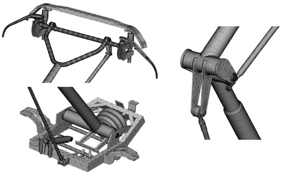
Surface meshes of pantograph model.

Figure 12.

Volume meshes of pantograph model.

To understand the propagation noise coming from the pantograph of the operational high-speed train using numerical simulation, it is important that the simulation condition be the same as the actual operating conditions. In particular, the inlet velocity must be equal to the actual train speed. The maximum speed of the high-speed train in South Korea is 300 km/h (83.3 m/s). Therefore, this study focused on the effects of the pantograph on flow-induced noise at an incoming flow speed of 83.3 m/s, as shown in Figure 13.

Figure 13.

Boundary conditions for simulation.

The numerical simulation of the pantograph model was conducted using the LBM implemented in the software PowerFLOW. The physical time scaling was 1.649 × 10⁻⁶ s and the simulation duration was 363,964 time steps. The time step of the analysis was related to the frequency ranges to be analyzed. The frequency range of the analysis was up to 3000 Hz, and the time step was selected by considering the aliasing effect. The noise generated from the pantograph is closely related to the time derivative of pressure in the flow field. In this sense, large pressure fluctuations occurred at the locations of the panhead, joint, and base sections, as shown in Figure 14. Moreover, it can be seen that complex turbulent flows were generated through the panhead, joint, and base sections. In particular, complicated vortexes were observed in the collector head, slide plate, and guide horn of the pantograph, as shown in Figure 15.

Figure 14.

Time derivative of pressure in pantograph.

Figure 15.

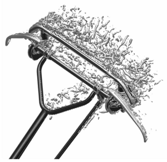
Vortex shedding of panhead.

The noise analysis position in the pantograph model was selected as shown in Figure 16. To analyze the propagation noise in the panhead, joint, and base sections, measurement locations were selected at 2 m from the center of each model. First, the sound pressure level in the propagation noise from the panhead section ranged from 102.3 to 107.6 dB(A) as shown in Figure 17. In addition, a high noise was generated from the back of the panhead through the flow. Moreover, it was confirmed that the highest noise was generated in almost all frequency ranges from 20 to 10,000 Hz, as shown in Figure 18. The frequency range of the dominant noise was from 200 to 800 Hz. Furthermore, it is noteworthy that the peak at 242 Hz occurred in the upper direction of the panhead. To investigate the noise generation mechanism, DNS using a two-dimensional panhead was conducted. The flow in the panhead section had continuous vortex sheddings, as shown in Figure 19. Moreover, the peak of the sound pressure about the two-dimensional panhead in the considered frequency range was at the same frequency of 242 Hz as the upper direction of the panhead, as shown in Figure 20. Therefore, the cause of the peak noise at 242 Hz was the vortex shadings of the panhead. Moreover, the same mechanism was also observed in the bandpass-filtered sound pressure between 200 and 300 Hz, as shown in Figure 21. The noise generated from the slide plate was that generated between 600 and 700 Hz, observed in the bandpass-filtered sound pressure.

Figure 16.

Noise measurement positions of pantograph.

Figure 17.

Sound pressure level of propagation noise from panhead section.

Figure 18.

Noise characteristics of panhead section.

Figure 19.

Direct numerical simulation of two-dimensional panhead section.

Figure 20.

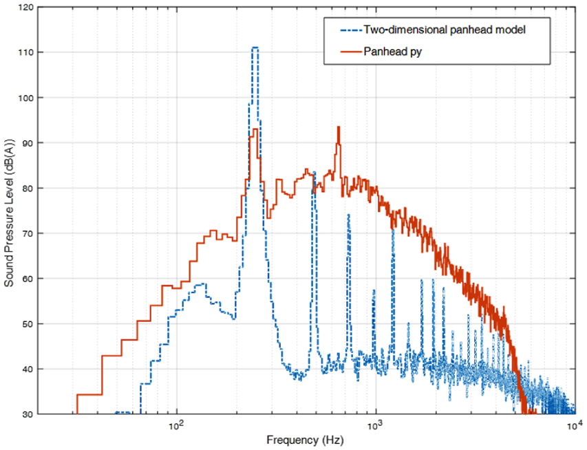
Noise characteristics of two-dimensional panhead model.

Figure 21.

Bandpass-filtered sound pressure derivation.

The sound pressure level generated from the joint section was between 90.3 and 103.5 dB(A), as shown in Figure 22. At the joint section, the noise spreading to both sides was larger than back and forth in the direction of the flow. The dominant noise frequency range was between 200 and 800 Hz, as shown in Figure 23. The sound pressure level generated from the base section was between 99.8 and 104.9 dB(A), as shown in Figure 24. The base section had the noise spreading to both sides in the direction of the flow. Moreover, the dominant noise in the frequency range was between 600 and 700 Hz, as shown in Figure 25.

Figure 22.

Sound pressure level of propagation noise from joint section.

Figure 23.

Noise characteristics of joint section.

Figure 24.

Sound pressure level of propagation noise from base section.

Figure 25.

Noise characteristics of base section.

Field test analysis

The purpose of this study is to identify the noise generation mechanism of the pantograph in a high-speed train. The main noise sources in the pantograph can be considered as complex aerodynamic flows around the structure when running at high speeds. However, it is difficult to derive the pantograph noise from the noise of the whole train when running at high speeds. Therefore, in this study, sound visualization results of the high-speed train were used to compare the propagation noise from the pantograph in the up and down modes under the same operational conditions as in a real high-speed train. The microphone array system has 144 channels and a spiral configuration, as shown in Figure 26. The measurement location was an open field in the Honam high-speed rail. Korean high-speed trains generally run at the maximum operating speed of 300 km/h. Therefore, the simulation analysis was carried out at the maximum operating speed. However, the tested high-speed train was designed to reach a speed higher than that of the conventional high-speed train. In particular, this train was able to run in the down mode of the pantograph in the operation line. Under this running condition, the high-speed train traveled without power supplied from the catenary. In order to distinguish the pantograph noise from the noise of the whole train when running at high speed, the propagation noise was measured from the pantograph in the up and down modes. The experiment was performed under the same conditions of vehicle speed, rail roughness, and measurement positions, which are the main factors affecting propagation noise.²³

Figure 26.

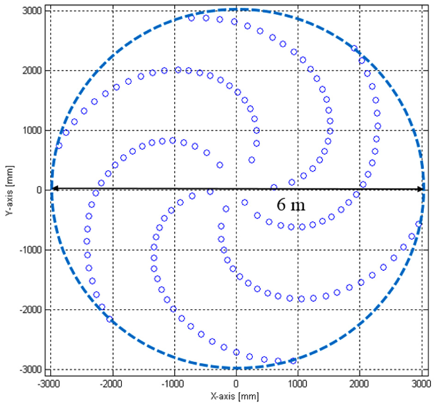
The 144-channel microphone array configuration.

The microphone used for the measurement was a 378B02 from PCB Piezotronics. The sampling rate was 12,800 Hz and data acquisition was PXI DAQ of National Instruments. The two photo sensors were used as start and end triggers to measure the speed of the train. The microphone array was located at 8 m from the rail center, as shown in Figure 27.

Figure 27.

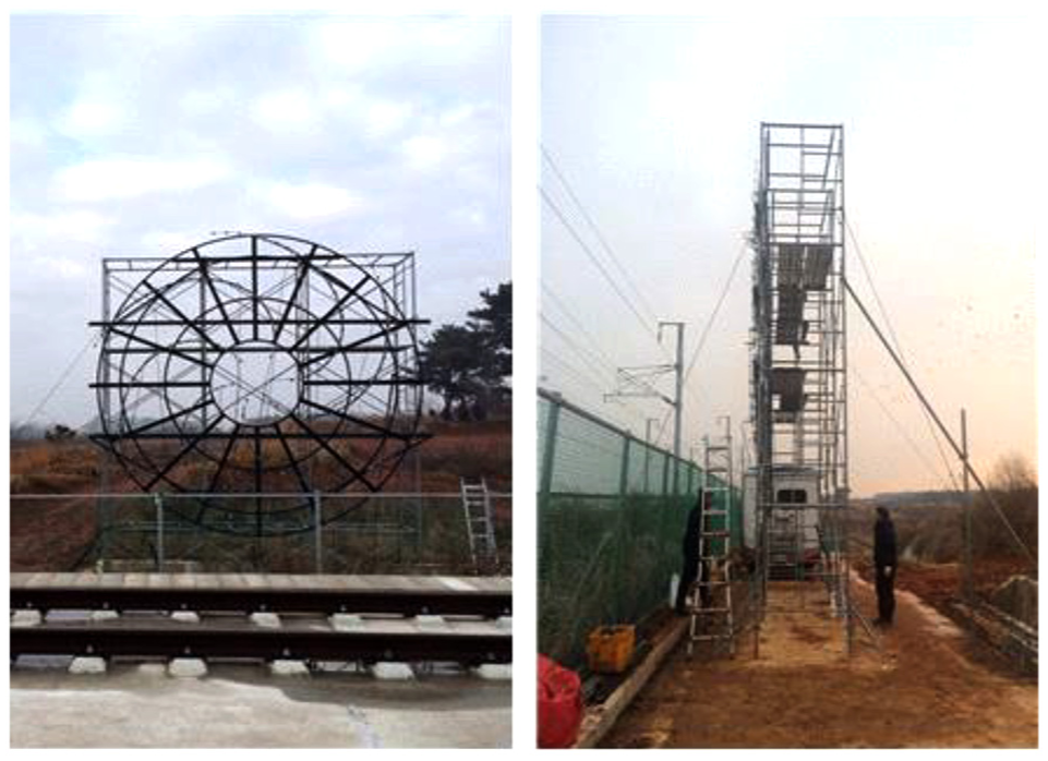
Microphone array measurement.

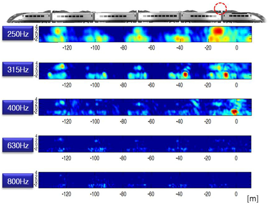
From the noise mapping results of the pantograph in the up mode at 350 km/h, the main noise sources such as wheels, inter-coach spacing, and pantograph are shown in Figure 28. Noise mapping results of the pantograph in the down mode at 350 km/h are shown in Figure 29. This measurement was carried out under the same conditions except for the pantograph being down. Moreover, because the pantograph, in the down mode, was in the pantograph cover area, it was difficult to generate aerodynamic noise from the structure. According to the two comparison results of exterior noise measurements using the microphone array, the noise of the pantograph was dominant in the low-frequency range, below 800 Hz. As a result of the simulation, it can be confirmed that the low-frequency noise is generated in the pantograph.

Figure 28.

Noise map of pantograph up at 350 km/h.

Figure 29.

Noise map of pantograph down at 350 km/h.

Conclusion

In this study, the aeroacoustic performances of the pantograph in a high-speed train were investigated through numerical analysis using the LBM. In the simulation analysis, a real-scaled pantograph was modeled and an incoming flow speed of 83.3 m/s was applied to examine the actual operational conditions of high-speed trains. From the simulation results, it was concluded that the highest noise was generated from the back of the pantograph through the flow in the frequency range from 200 to 800 Hz. Moreover, the dominant noise sources in the pantograph were the panhead, joint, and base sections. In particular, the simulation analysis showed that the peak noise of the panhead was the vortex shadings through the flows. In this sense, this study proposes the detailed noise generation mechanism of the pantograph that is essential for effectively reducing the aerodynamic noise of the pantograph.

Footnotes

Appendix 1

Handling Editor: Ahmed Abdel Gawad

Declaration of conflicting interests

The author(s) declared no potential conflicts of interest with respect to the research, authorship, and/or publication of this article.

Funding

The author(s) disclosed receipt of the following financial support for the research, authorship, and/or publication of this article: This research was supported by a grant from R&D Program of the Korea Railroad Research Institute, Republic of Korea.

ORCID iD

Hee-Min Noh

References

Thompson

. Railway noise and vibration: mechanisms, modelling and means of control. 1st ed. Oxford: Elsevier, 2009.

Noh

H-M

Choi

Hong

et al . Investigation of noise sources in high-speed trains. P I Mech Eng F: J Rai 2014; 228: 307–322.

Poisson

Gautier

Letourneaux

. Noise sources for high speed trains: a review of results in the TGV case. In: Schulte-Werning

(ed.) Noise and vibration mitigation for rail transportation systems: notes on numerical fluid mechanics and multidisciplinary design, vol. 99. Berlin; Heidelberg: Springer, 2008, pp.71–77.

Noh

H-M

Choi

J-W

. Identification of low-frequency noise sources in high-speed train via resolution improvement. J Mech Sci Technol 2015; 29: 3609–3615.

Kook

Moebs

Davies

et al . An efficient procedure for visualizing the sound field radiated by vehicles during standardized pass-by tests. J Sound Vib 2000; 233: 137–156.

Mellet

Letournearux

Poisson

et al . High speed train noise emission: latest investigation of the aerodynamic/rolling noise contribution. J Sound Vib 2006; 293: 535–546.

Zhu

Thompson

. Flow simulation and aerodynamic noise prediction for a high-speed train wheelset. Int J Aeroacoust 2014; 13: 533–552.

Zhu

Thompson

. Flow behaviour and aeroacoustic characteristics of a simplified high-speed train bogie. P I Mech Eng F: J Rai 2016; 230: 1642–1658.

Marie

Ricot

Sagaut

. Comparison between lattice Boltzmann method and Navier-Stokes high order schemes for computational aeroacoustics. J Comput Phys 2009; 228: 1056–1070.

10.

Chen

Doolen

. Lattice Boltzmann method for fluid flows. Annu Rev Fluid Mech 1998; 30: 329–364.

11.

Ricot

Maillard

Bailly

. Numerical simulation of unsteady cavity flow using lattice Boltzmann method. In: Proceedings of the 8th AIAA/CEAS aeroacoustics conference and exhibit, Breckenridge, CO, 17–19 June 2002, pp.2002–2532. Reston, VA: American Institute of Aeronautics and Astronautics.

12.

Casalino

Riberiro

AFP

Fares

. Facing rim cavities fluctuation modes. J Sound Vib 2014; 333: 2812–2830.

13.

Bhatnagar

Gross

Krook

. A model for collision processes in gases—I: small amplitude processes in charged and neutral one-component systems. Phys Rev J Arch 1954; 94: 511–525.

14.

Frisch

Hasslacher

Pomeeau

. Lattice-gas automata for the Navier-Stokes equation. Phys Rev Lett 1986; 56: 1505–1508.

15.

Chen

Matthaeus

. Recovery of the Navier-Stokes equations using a lattice-gas Boltzmann method. Phys Rev A 1992; 45: R5339–R5342.

16.

Chen

Orszag

Staroselsky

et al . Expanded analogy between Boltzmann kinetic theory of fluids and turbulence. J Fluid Mech 2003; 519: 301–314.

17.

Chen

Kandasamy

Orszag

et al . Extended Boltzmann kinetic equation for turbulent flows. Science 2003; 301: 633–636.

18.

Yakhot

Orszag

. Renormalization group analysis of turbulence—I: basic theory. J Sci Comput 1986; 1: 3–51.

19.

Exa Corporation. PowerFLOW user’s guide, release 4.4. Boston, MA: Exa Corporation, 2011.

20.

Chen

Teixeira

Movig

. Realization of fluid boundary conditions via discrete Boltzmann dynamics. Int J Mod Phys C 1998; 9: 1281–1292.

21.

Revell

Prydz

Hays

. Experimental study of airframe noise vs. drag relationship for circular cylinders. Lockheed Report 28074, Final Report NASA Contract NAS1–14403, February 1977. Washington, DC: National Aeronautics and Space Administration.

22.

Orselli

Meneghini

Saltara

. Two and three-dimensional simulation of sound generated by flow around a circular cylinder. In: Proceedings of the 15th AIAA/CEAS aeroacoustics conference (30th AIAA aeroacoustics conference), Miami, FL, 11–13 May 2009. Reston, VA: American Institute of Aeronautics and Astronautics.

23.

Noh

H-M

Kim

J-K

et al . Noise contribution analysis of pantograph using real train experiment. J Korean Soc Rail 2016; 19: 271–279.

Numerical analysis of aerodynamic noise from pantograph in high-speed trains using lattice Boltzmann method

Abstract

Keywords

Introduction

LBM

Verification of computational method

Numerical analysis of pantograph

Field test analysis

Conclusion

Footnotes

Appendix 1

Declaration of conflicting interests

Funding

ORCID iD

References