Numerical analysis of stochastic SIR model by Legendre spectral collocation method

Abstract

This article represents Legendre spectral collocation method based on Legendre polynomials to solve a stochastic Susceptible, infected, Recovered (SIR) model. The Legendre polynomials on stochastic SIR model that convert it to a system of equations has been applied and then solved by the Legendre spectral method, which leads to excellent accuracy and convergence by implementing Legendre–Gauss–Lobatto collocation points permitting to generate coarser meshes. The numerical results for both the deterministic and stochastic models are presented. In case of probably small noise, the verge dynamics is analyzed. The large noise will show eradication of disease, which controls disease spreading. Various graphical results demonstrate the effectiveness of the proposed method to SIR model.

Introduction

There are many classical epidemic models which have been intentional and recommended for modeling of spread process of the infectious diseases, like Susceptible, infected, Recovered (SIR), Susceptible infected, Recovered, Susceptible (SIRS), and Susceptible, Exposed, infected Recovered models. These models have been proposed by many researchers to study the dynamics of disease spread and controls.^1–9

Mathematical modeling of infectious diseases has an old history. In 1760, an infectious disease model was proposed by Bernoulli ¹⁰ for smallpox. Furthermore, in 1906, H Hamer ¹¹ studied the measles epidemic through an SIR model. After that, a mathematical model was proposed by RA Ross ¹² in 1911 to study the dynamics of malaria. The models proposed in previous studies^13–16 were used in a different way for different disease dynamics. Moreover, the first classical SIR model was proposed by WO Kermack and AG McKendrick, ¹⁷ where the population is considered in three compartments, that is susceptible, infected, and recovered.

Susceptible becomes infected, and infected becomes recovered, is the concept of SIR model. However, for some epidemic diseases, the recovery does not produce lifelong protection, for example, plague, meningitis, malaria, and sleeping sickness; ¹⁸ thus, susceptible persons are individually transferred to the infected persons and then consequently to recovery, and return to susceptible class, such type of model is identified as Susceptible, Infected, Susceptible (SIS) model. The SIS model has been studied by many researchers.^19–21 Although for some epidemic diseases, the recovery can produce protection for the time being, and after some time, recovery may lose protection and returns to the susceptible class, such as influenza, smallpox, tetanus, typhoid fever, and cholera. Such type of model is called SIRS model. Literature^22–24 is full of many research papers which are based on SIR models. These SIR models have been proposed by the authors for a specific infectious disease with specific incident rate.

Using the Legendre spectral collocation method (LSCM), we prepared an SIR model with stochastic effect to present their numerical solution. There is no such article in the literature that shows the dynamics of an SIR stochastic model. So, this is a novel approach to study stochastic SIR model. The nonlinear SIR model is as follows

$$(\begin{array}{c}\frac{\mathrm{dS}(t)}{\mathrm{dt}}=\mathrm{\Lambda }-\beta S(t)I(t)-\mu S(t)+\epsilon I(t)\hfill \\ \frac{\mathrm{dI}(t)}{\mathrm{dt}}=\beta S(t)I(t)-(\mu +\epsilon +\gamma )I(t)\hfill \\ \frac{\mathrm{dR}(t)}{\mathrm{dt}}=\gamma I(t)-\mu R(t)\hfill \end{array}$$

(1)

Total population $N$ are categorized further into three classes, these classes are represented by $S(t),I(t),R(t)$ . In equation (1), $S(t)$ represents the population of susceptible individuals, $I(t)$ denotes the population of infected individuals, and $R(t)$ is the population of recovered individuals. The parameters $\mathrm{\Lambda },\beta ,\epsilon ,\mu$ , and $\gamma$ are positive constants. Parameter $\mathrm{\Lambda }$ represents the natural birth rate of susceptible individuals, $\mu$ represents natural death rate in each individuals class, disease contact rate is given by $\beta$ , $\gamma$ denotes recovery rate of infected individuals, and the infected individuals become susceptible at a rate $\epsilon$ and move to susceptible class. Using LaSalle’s invariance principle, a threshold dynamics of equation (1) is driven by basic reproduction number $R_0$ ; therefore, if the reproduction number $R_0<1$ , then equation (1) has infection-free equilibrium $E_0=(\mathrm{\Lambda }/\mu ,0,0)$ and asymptotically stable. However, if the reproduction number $R_0>1$ , then endemic equilibrium $E^{*}=(S^{*},I^{*},R^{*})$ of the given system is asymptotically stable. ²⁵

The stochastic perturbations are assumed to be white noise, and the system equation (1) will be deduced to the following form

$$(\begin{array}{c}\mathrm{dS}(t)=(\mathrm{\Lambda }-\beta S(t)I(t)-\mu S(t)+\epsilon I(t))\mathrm{dt}+\sigma S(t)\mathrm{dW}(t)\hfill \\ \multicolumn{1}{c}{\mathrm{dI}(t)=(\beta S(t)I(t)-(\mu +\epsilon +\gamma )I(t))\mathrm{dt}+\sigma I(t)\mathrm{dW}(t)}\\ \multicolumn{1}{c}{\mathrm{dR}(t)=(\gamma I(t)-\mu R(t))\mathrm{dt}+\sigma R(t)\mathrm{dW}(t)}\end{array}$$

(2)

where $S(0)={\alpha }_1,I(0)={\alpha }_2,\mathrm{and}R(0)={\alpha }_3$ are the initial conditions, $W(t)$ are the Brownian motions, and each ${\sigma }^2>0$ is the intensity of $W(t)$ . The aim of this study is to implement present method for numerical solution of stochastic SIR model given in equation (2). This method was previously demonstrated by D Lehotzky et al., ²⁶ for the stability analysis of time-periodic delay-differential equations with multiple and distributed delays. Similarly, P Zakian and N Khaji ²⁷ discussed the stochastic spectral finite element method for wave propagation analysis with medium uncertainties. The Legendre polynomials have been used by many researchers for approximate solution of differential and integral equations.^28,29

This article is structured as follows: Legendre polynomials are reviewed in section “Legendre polynomials.” In section “Description of LSCM,” a brief description of LSCM is given to solve equation (2). Analysis is given in section “Analysis of stochastic SIR model.” Numerical results are discussed in section “Numerical results.” The conclusion is given in section “Conclusion.”

Legendre polynomials

In this section, we review the Legendre polynomials; the N-order Legendre polynomials are denoted by $P_N(t)$ . Any function $x(t)$ defined over $[-1,1]$ can be approximated by Legendre interpolating polynomials as

$$x(t)=\sum _{n=0}^N{x}_n{P}_n(t)$$

(3)

where $x_n=x(t_n)$ are unknown Legendre coefficients, $t_n,n=0,1,\dots ,N$ are interpolating points which satisfy $-1=t_0<t_1<\cdots <t_{N-1}<t_N=1$ , and $P_N(t)$ is the N-order Legendre polynomial defined by

$$\begin{array}{c}{P}_n(t)=\frac{1}{2^n}\sum _{k=0}^{\left[\frac{n}{2}\right]}(-1{)}^k\left(\begin{array}{c}n\\ k\end{array}\right)\left(\begin{array}{c}2n-2k\\ n\end{array}\right)t^{n-2k},t\in [-1,1]\hfill \\ (n=0,1,2,\dots ,N)\hfill \\ \left[\frac{n}{2}\right]=(\begin{array}{cc}\frac{n}{2},\hfill & n\mathrm{even}\hfill \\ \multicolumn{1}{c}{\frac{n-1}{2},}& n\mathrm{odd}\hfill \end{array}\hfill \end{array}$$

(4)

Description of LSCM

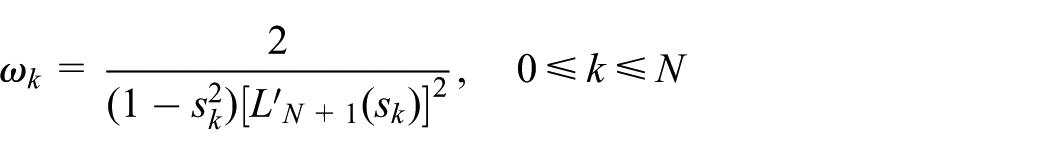
In this section, we introduce LSCM to solve stochastic SIR model defined in equation (2). In the procedure of LSCM, the Legendre–Guass quadrature with weight function has been used. For this method, we consider Legendre–Gauss–Lobatto points $\{t_j{\}}_{j=0}^N,$ ; therefore, roots of $L_{N+1}(t),$ where $L_{N+1}$ is $(N+1)\mathrm{th}$ Legendre polynomial.

Our purpose is to obtain an approximate solution of equation (2); for this, taking integral within $[0,t]$ on both sides of equation (2), then the equation takes the following form

$$\begin{array}{c}S(t)=S(0)+\underset{0}{\overset{t}{\int }}(\mathrm{\Lambda }-\beta S(s)I(s)-\mu S(s)+\epsilon I(s))\mathrm{ds}+\underset{0}{\overset{t}{\int }}\sigma S(s)\mathrm{dW}(s)\hfill \\ I(t)=I(0)+\underset{0}{\overset{t}{\int }}(\beta S(s)I(s)-(\mu +\epsilon +\gamma )I(s))\mathrm{ds}+\underset{0}{\overset{t}{\int }}\sigma I(s)\mathrm{dW}(s)\hfill \\ R(t)=R(0)+\underset{0}{\overset{t}{\int }}(\gamma I(s)-\mu R(s))\mathrm{ds}+\underset{0}{\overset{t}{\int }}\sigma R(s)\mathrm{dW}(s)\hfill \end{array}$$

(5)

where the initial conditions $S(0),I(0),R(0)$ , respectively, are of the functions of $S(t),I(t),R(t)$ . To analyzed LSCM on a standard interval of $[-1,1]$ , take linear transformation $s=t/2(\theta +1)$ , then equation (5) becomes

$$\begin{array}{c}\multicolumn{1}{c}{S(t)=S(0)+\frac{t}{2}\underset{-1}{\overset{1}{\int }}[\mathrm{\Lambda }-\beta S(\frac{t}{2}(\theta +1))I(\frac{t}{2}(\theta +1))-\mu S(\frac{t}{2}(\theta +1))+\epsilon I(\frac{t}{2}(\theta +1))]d\theta }\\ +\frac{t}{2}{\int }_{-1}^1\sigma S(\frac{t}{2}(\theta +1))\mathrm{dW}(\theta )\hfill \\ \multicolumn{1}{c}{I(t)=I(0)+\frac{t}{2}\underset{-1}{\overset{1}{\int }}[\beta S(\frac{t}{2}(\theta +1))I(\frac{t}{2}(\theta +1))-(\mu +\epsilon +\gamma )I(\frac{t}{2}(\theta +1))]d\theta }\\ +\frac{t}{2}\underset{-1}{\overset{1}{\int }}\sigma I(\frac{t}{2}(\theta +1))\mathrm{dW}(\theta )\hfill \\ \multicolumn{1}{c}{R(t)=R(0)+\frac{t}{2}\underset{-1}{\overset{1}{\int }}[\gamma I(\frac{t}{2}(\theta +1))-\mu R(\frac{t}{2}(\theta +1))]d\theta +\frac{t}{2}\underset{-1}{\overset{1}{\int }}\sigma R(\frac{t}{2}(\theta +1))\mathrm{dW}(\theta )}\end{array}$$

(6)

The semi-discretized spectral equations of equation (6) are

$$\begin{array}{c}\multicolumn{1}{c}{S(t)=S(0)+\frac{t}{2}\sum _{k=0}^N[\mathrm{\Lambda }-\beta S(\frac{t}{2}({\theta }_k+1))I(\frac{t}{2}({\theta }_k+1))-\mu S(\frac{t}{2}({\theta }_k+1))+\epsilon I(\frac{t}{2}({\theta }_k+1))]{\omega }_k}\\ +\frac{t}{2}\sum _{k=0}^N\left[\sigma S(\frac{t}{2}({\theta }_k+1))\right]{\omega }_k^{*}\hfill \\ \multicolumn{1}{c}{I(t)=I(0)+\frac{t}{2}\sum _{k=0}^N[\beta S(\frac{t}{2}({\theta }_k+1))I(\frac{t}{2}({\theta }_k+1))-(\mu +\epsilon +\gamma )I(\frac{t}{2}({\theta }_k+1))]{\omega }_k}\\ +\frac{t}{2}\sum _{k=0}^N\left[\sigma I(\frac{t}{2}({\theta }_k+1))\right]{\omega }_k^{*}\hfill \\ \multicolumn{1}{c}{R(t)=R(0)+\frac{t}{2}\sum _{k=0}^N[\gamma I(\frac{t}{2}({\theta }_k+1))-\mu R(\frac{t}{2}({\theta }_k+1))]{\omega }_k+\frac{t}{2}\sum _{k=0}^N\left[\sigma R(\frac{t}{2}({\theta }_k+1))\right]{\omega }_k^{*}}\end{array}$$

(7)

where Legendre–Gauss quadrature with weight function is

$${\omega }_k=\frac{2}{(1-s_k^2)[{L\prime }_{N+1}(s_k{)]}^2},0\le k\le N$$

Similarly, Legendre–Gauss quadrature with stochastic weight function is

$${\omega }_k^{*}=\sqrt{{\omega }_k}\times \mathrm{randn}(1,N),0\le k\le N$$

Now using Legendre polynomial to approximate $S(t),I(t)$ , and $R(t)$ using equation (3)

$$S(t)=\sum _{n=0}^N{S}_n{P}_n(t),I(t)=\sum _{n=0}^N{I}_n{P}_n(t),R(t)=\sum _{n=0}^N{R}_n{P}_n(t)$$

(8)

where $S_n=S(t_n),I_n=I(t_n),R_n=R(t_n)$ are Legendre coefficients to the functions $S(t),I(t)$ , and $R(t)$ , respectively. Now using above approximation equation (2), the equation can be reduced to the following form

$$\begin{array}{cc}\multicolumn{1}{c}{\sum _{n=0}^N{S}_n{P}_n(t)=}& \sum _{n=0}^N{S}_n{P}_n(0)+\frac{t}{2}\sum _{k=0}^N[\mathrm{\Lambda }-\beta \sum _{n=0}^N{S}_n{P}_n({\eta }_k)\sum _{n=0}^N{I}_n{P}_n({\eta }_k)-\mu \sum _{n=0}^N{S}_n{P}_n({\eta }_k)\hfill \\ \multicolumn{1}{c}{}& +\epsilon \sum _{n=0}^N{I}_n{P}_n({\eta }_k)]{\omega }_k+\frac{t}{2}\sum _{k=0}^N[\sigma \sum _{n=0}^N{S}_n{P}_n({\eta }_k)]{\omega }_k^{*}\hfill \\ \multicolumn{1}{c}{\sum _{n=0}^N{I}_n{P}_n(t)=}& \sum _{n=0}^N{I}_n{P}_n(0)+\frac{t}{2}\sum _{k=0}^N[\beta \sum _{n=0}^N{S}_n{P}_n({\eta }_k)\sum _{n=0}^N{I}_n{P}_n({\eta }_k)-(\mu +\epsilon +\gamma )\sum _{n=0}^N{I}_n{P}_n({\eta }_k)]{\omega }_k\hfill \\ \multicolumn{1}{c}{}& +\frac{t}{2}\sum _{k=0}^N[\sigma \sum _{n=0}^N{I}_n{P}_n({\eta }_k)]{\omega }_k^{*}\hfill \\ \multicolumn{1}{c}{\sum _{n=0}^N{R}_n{P}_n(t)=}& \sum _{n=0}^N{R}_n{P}_n(0)+\frac{t}{2}\sum _{k=0}^N[\gamma \sum _{n=0}^N{I}_n{P}_n({\eta }_k)-\mu \sum _{n=0}^N{R}_n{P}_n({\eta }_k)]{\omega }_k\hfill \\ \multicolumn{1}{c}{}& +\frac{t}{2}\sum _{k=0}^N[\sigma \sum _{n=0}^N{R}_n{P}_n({\eta }_k)]{\omega }_k^{*}\hfill \end{array}$$

(9)

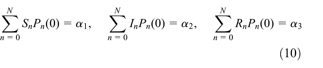
For simplicity, ${\eta }_k=(t/2({\theta }_k+1))$ . Thus, the system equation (9) contains $3N+3$ number of unknowns with $3N$ nonlinear algebraic equations. Also using the initial conditions

$$\sum _{n=0}^N{S}_n{P}_n(0)={\alpha }_1,\sum _{n=0}^N{I}_n{P}_n(0)={\alpha }_2,\sum _{n=0}^N{R}_n{P}_n(0)={\alpha }_3$$

(10)

Thus, equations (9) and (10) form a system of $(3N+3)$ nonlinear algebraic equations with $(3N+3)$ unknowns for $S_n,I_n,R_n$ for $n=0,1,\dots ,N$ . This system obtains the unknowns $S_n,I_n,R_n$ , $n=0,1,\dots ,N$ , by substituting the value of unknowns in equations $(8)-(10)$ ; then, we obtain an approximate solution to the stochastic SIR model equation (2).

Analysis of stochastic SIR model

We consider both deterministic SIR model equation (1) and stochastic SIR model equation (2) with saturated incident rate $\beta S(t)I(t)$ . For equation (1), the reproduction number is defined by $R_0=\mathrm{\Lambda }\beta /\mu (\mu +\epsilon +\gamma )$ and then the following theorems are considered.

Theorem 1

If $R_0<1$ , then solution of system equation (1) has infection-free equilibrium $E_0=(\mathrm{\Lambda }/\mu ,0,0)$ . If reproduction $R_0>1$ , then system equation (1) has a unique endemic equilibrium $E^{*}=(S^{*},I^{*},R^{*})$ , where

$$S^{*}=\frac{(\mu +\epsilon +\gamma )}{\beta },I^{*}=\frac{(\mathrm{\Lambda }\beta -\mu (\mu +\epsilon +\gamma ))}{\beta (\mu +\gamma )},R^{*}=\frac{\gamma I^{*}(t)}{\mu }$$

Proof

Let $E^{*}$ be endemic equilibrium of system equation (1), then $S^{*},I^{*},R^{*}$ must satisfy the following system

$$\begin{array}{c}\mathrm{\Lambda }-\beta S^{*}(t)I^{*}(t)-\mu S^{*}(t)+\epsilon I^{*}(t)=0\hfill \\ \beta S^{*}(t)I^{*}(t)-(\mu +\epsilon +\gamma )I^{*}(t)=0\hfill \\ \gamma I^{*}(t)-\mu R^{*}(t)=0\hfill \end{array}$$

(11)

To prove the system equation (11), we considering the two cases: $I^{*}(t)=0$ and $I^{*}(t)>0$ :

• $I^{*}(t)=0$ : from last equation of equation (11), we get, $R^{*}(t)=0$ , and from first equation of equation (11), $S^{*}(t)=\mathrm{\Lambda }/\mu$ . Hence, we can get $E_0=(\mathrm{\Lambda }/\mu ,0,0)$ , which is disease-free equilibrium. In this case, the reproduction number $R_0<1$ .

• $I^{*}(t)>0$ : from last equation array of equation (11), we get

$$R^{*}=\frac{\gamma I^{*}(t)}{\mu }$$

Using the value of $R^{*}$ in second equation array of equation (11), then we get

$$S^{*}=\frac{(\mu +\epsilon +\gamma )}{\beta }$$

Then, substituting the above equations into the first equation array of equation (11), we get a unique root

$$I^{*}=\frac{(\mathrm{\Lambda }\beta -\mu (\mu +\epsilon +\gamma ))}{\beta (\mu +\gamma )}$$

If $I^{*}>0$ , we must have $\beta \mathrm{\Lambda }>\mu (\mu +\epsilon +\gamma )$ , it means that $R_0>1$ . This completes the proof of theorem.

Note that throughout in this article, we assume that $R^r$ is the r-dimensional Euclidean space and also $R_{+}^r:=x\in R^r:x_j>0,1\le j\le r$ .

Lemma 1

The region $\Pi =\{(S(0),I(0),R(0))\in R_{+}^3:S(t)>0,I(t)>0,R(t)>0,S(t)+I(t)+R(t)\le \mathrm{\Lambda }/\mu \}$ is a positively invariant set for system equation (2).

Proof

Since total population is defined by $N(t)=S(t)+I(t)+R(t)$ , then by system equation (2), we get

$$\frac{\mathrm{dN}(t)}{\mathrm{dt}}=\mathrm{\Lambda }+(\sigma -\mu )N(t)$$

Therefore

$$\begin{array}{cc}\multicolumn{1}{c}{N(t)}& =\frac{\mathrm{\Lambda }}{\mu -\sigma }+N(0)e^{(\sigma -\mu )t}\hfill \\ \multicolumn{1}{c}{}& \le \frac{\mathrm{\Lambda }}{\mu }+N(0)e^{(\sigma -\mu )t}\hfill \\ \multicolumn{1}{c}{}& \le \frac{\mathrm{\Lambda }}{\mu }\hfill \end{array}$$

Thus, for system equation (2), the region $\Pi$ is positively invariant.

Using method from Meng et al., ¹⁴ the following lemma can be proved.

Lemma 2

The solution of system equation (2) $(S(t),I(t),R(t))$ has following properties for each $(S(0),I(0),R(0))\in R_{+}^3$

$$\begin{array}{c}\underset{t\to \infty }{lim}\frac{1}{t}\underset{0}{\overset{t}{\int }}\sigma S(s)\mathrm{dW}(s)=0,\underset{t\to \infty }{lim}\frac{1}{t}\underset{0}{\overset{t}{\int }}\sigma I(s)\mathrm{dW}(s)=0,\hfill \\ \underset{t\to \infty }{lim}\frac{1}{t}\underset{0}{\overset{t}{\int }}\sigma R(s)\mathrm{dW}(s)=0\hfill \end{array}$$

Definition 1

For system equation (2), the infected persons I(t) are called extinctive if ${lim}_{t\to \infty }I(t)=0$ .

Theorem 2

For the $max\{\beta \mu /\mathrm{\Lambda },{\beta }^2/2(\mu +\epsilon +\gamma )\}<{\sigma }^2$ or $\beta \mu /\mathrm{\Lambda }>{\sigma }^2$ with ${\overline{R}}_0<1$ , the infected class $I(t)$ of system equation (2) exponentially tends to zero. Consequently, for ${\overline{R}}_0>1$ , then $I(t)$ is present in equation (2), where

$${\overline{R}}_0=R_0-\frac{{\sigma }^2{\mathrm{\Lambda }}^2}{2{\mu }^2(\mu +\epsilon +\gamma )}$$

Proof

Let $(S(t),I(t),R(t))$ is the solution of system equation (2) satisfying the initial values $(S(0),I(0),R(0))\in R_{+}^3$ . Then, by $\hat{o}$ formula

$$\begin{array}{cc}\multicolumn{1}{c}{d\ln I(t)}& =(\beta S(t)-(\mu +\epsilon +\gamma )\hfill \\ \multicolumn{1}{c}{}& -\frac{1}{2}{\sigma }^2{S}^2(t))\mathrm{dt}+\sigma S(t)\mathrm{dW}(t)\hfill \end{array}$$

(12)

Taking integral of system equation (12) within $[0,1]$ , then

$$\begin{array}{cc}\multicolumn{1}{c}{\ln I(t)=}& \ln I(0)+\underset{0}{\overset{t}{\int }}(\beta S(t)-(\mu +\epsilon +\gamma )\hfill \\ \multicolumn{1}{c}{}& -\frac{1}{2}{\sigma }^2{S}^2(t))\mathrm{dt}+\underset{0}{\overset{t}{\int }}\sigma S(t)\mathrm{dW}(t)\hfill \end{array}$$

(13)

Now, we have to discuss two cases: whether ${\sigma }^2>\beta \mu /\mathrm{\Lambda }$ or not; then, equation (13) takes the form

$$\begin{array}{cc}\multicolumn{1}{c}{\ln I(t)}& \le \ln I(0)+(\frac{{\beta }^2}{{\sigma }^2}-(\mu +\epsilon +\gamma ))t\hfill \\ \multicolumn{1}{c}{}& +\underset{0}{\overset{t}{\int }}\sigma S(t)\mathrm{dW}(t)\hfill \end{array}$$

(14)

Dividing both sides of equation (14) by $t>0$ , then

$$\begin{array}{cc}\multicolumn{1}{c}{\frac{\ln I(t)}{t}}& \le \frac{1}{t}\ln I(0)-(\mu +\epsilon +\gamma -\frac{{\beta }^2}{{\sigma }^2})\hfill \\ \multicolumn{1}{c}{}& +\frac{1}{t}\underset{0}{\overset{t}{\int }}\sigma S(t)\mathrm{dW}(t)\hfill \end{array}$$

(15)

Taking ${lim}_{t\to \infty }$ and using Lemma 2, then equation (15) takes the following form

$$\underset{t\to \infty }{lim}\frac{\ln I(t)}{t}\le -(\mu +\epsilon +\gamma -\frac{{\beta }^2}{{\sigma }^2})<0$$

Similarly, ${\sigma }^2>{\beta }^2/2(\mu +\epsilon +\gamma )$ , which shows that ${lim}_{t\to \infty }I(t)=0.$ If ${\sigma }^2<\beta \mu /\mathrm{\Lambda }$ , then from equation (13), we have

$$\begin{array}{cc}\multicolumn{1}{c}{\ln I(t)}& \le \ln I(0)+(\frac{\beta \mathrm{\Lambda }}{\mu }-\frac{{\sigma }^2{\mathrm{\Lambda }}^2}{2{\mu }^2}-(\mu +\epsilon +\gamma ))t\hfill \\ \multicolumn{1}{c}{}& +\underset{0}{\overset{t}{\int }}\sigma S(t)\mathrm{dW}(t)\hfill \end{array}$$

(16)

Dividing both sides of equation (16) by $t>0$ , we obtain

$$\begin{array}{c}\frac{1}{t}\ln I(t)\le \frac{1}{t}\ln I(0)+(\mu +\epsilon +\gamma )\hfill \\ (\frac{\beta \mathrm{\Lambda }}{\mu (\mu +\epsilon +\gamma )}-\frac{{\sigma }^2{\mathrm{\Lambda }}^2}{2{\mu }^2(\mu +\epsilon +\gamma )}-1)\hfill \\ +\frac{1}{t}\underset{0}{\overset{t}{\int }}\sigma S(t)\mathrm{dW}(t)\hfill \end{array}$$

(17)

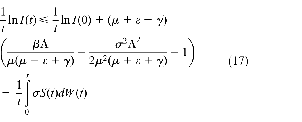
Again taking ${lim}_{t\to \infty }$ and using Lemma 2, equation (15) takes the form

$$\underset{t\to \infty }{lim}\frac{\ln I(t)}{t}\le ({\overline{R}}_0-1)(\mu +\epsilon +\gamma )$$

For ${\overline{R}}_0<1$

$$\underset{t\to \infty }{lim}\frac{\ln I(t)}{t}<0$$

which shows that ${lim}_{t\to \infty }I(t)=0$ . Consequently, if ${\overline{R}}_0>1$ , then

$$\underset{t\to \infty }{lim}\frac{\ln I(t)}{t}>0$$

This completes the proof of the theorem.

Numerical results

We perform numerical results of stochastic SIR models given in equations (1) and (2) for different parameter values to show the efficiency and simplicity of LSCM. The associated computations were performed using Maple and MATLAB on a personal computer.

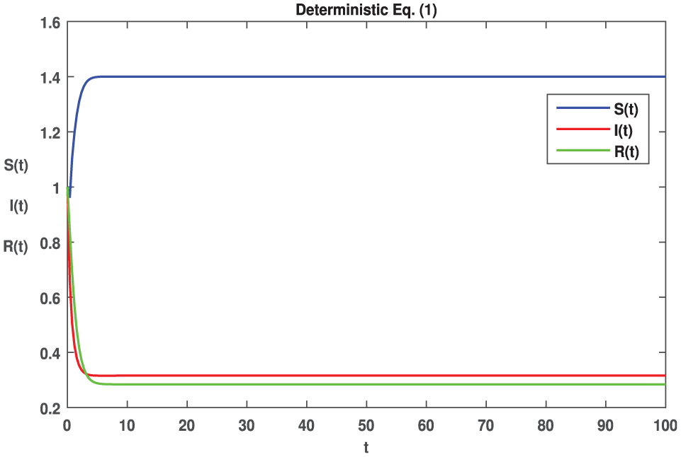
First, we set initial conditions $S(0)=1,I(0)=1,R(0)=1$ . Then, we give the appropriate parameter values $\mathrm{\Lambda }=2,\beta =1,\mu =1,\epsilon =0.9,\gamma =0.9$ , for deterministic system equation (1). Using above parameters, the computation shows that reproduction number $R_0=0.714286<1$ , using Theorem 1, we clearly see that system equation (1) has stable disease-free equilibrium $E_0(2,0,0)$ , where the susceptible individuals are clearly equal to $\mathrm{\Lambda }/\mu =2$ ; this dissertation is shown in Figure 1.

Figure 1.

Time series for the solution of deterministic SIR system equation (1), with $\mathrm{\Lambda }=2,\beta =1,\mu =1,\gamma =0.9,\epsilon =0.9$ , where $R_0=0.714286<1$ and $E_0(2,0,0)$ .

While if we take $\beta =2$ and the same remaining parameter values of Figure 1, then the reproduction $R_0=1.428571>1$ ; again using Theorem 1, the simple calculation is made in this case and found that the system equation (1) has stable infectious equilibrium $E^{*}(1.4,0.315789,0.284211)$ ; therefore, the susceptible individuals have $S^{*}(t)=1.4$ , and infected and recoverable individuals have $I^{*}(t)=0.315789$ and $R^{*}(t)=0.284211$ , respectively, which is shown Figure 2.

Figure 2.

Time series for the solution of deterministic SIR system equation (1), with $\mathrm{\Lambda }=2,\beta =2,\mu =1,\gamma =0.9,\epsilon =0.9$ , where $R_0=1.428571>1$ and $E^{*}(1.4,0.315789,0.284211)$ .

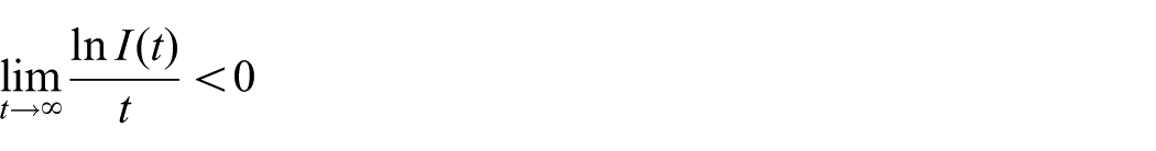
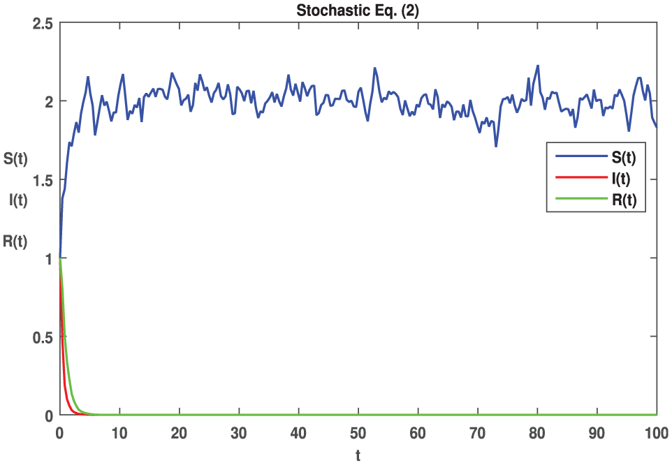
If we choose $\sigma =0.5$ and the parameter values $\mathrm{\Lambda }=2,\beta =1,\mu =1,\epsilon =0.9,\gamma =0.9$ , for deterministic system equation (2), then the simple calculation shows the condition ${\sigma }^2<max\{\beta \mu /\mathrm{\Lambda },{\beta }^2/2(\mu +\epsilon +\gamma )\}$ , and ${\overline{R}}_0=0.535715<1$ ; then, by Theorem 2, the infected individuals of system equation (2) tend to zero, and this can shown in Figure 3, and we clearly see that $I(t)$ approaches to zero.

Figure 3.

Time series for the solution of stochastic SIR system equation (2), with $\mathrm{\Lambda }=2,\beta =1,\mu =1,\gamma =0.9,\epsilon =0.9,\sigma =0.5$ , where ${\sigma }^2<max\{\beta \mu /\mathrm{\Lambda },{\beta }^2/2(\mu +{\rho }_1+{\rho }_2+\alpha )\}$ and ${\overline{R}}_0=0.535715<1$ .

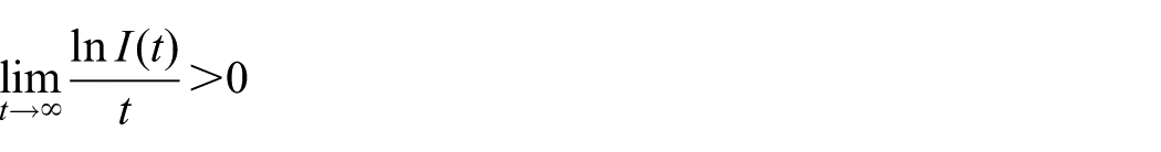
Similarly, if we choose $\beta =2,$ with intensity of noise $\sigma =0.5$ and the same remaining parameter values as in Figure 3, then the simple calculation shows that the deterministic system equation (2) satisfies the condition ${\sigma }^2<max\{\beta \mu /\mathrm{\Lambda },{\beta }^2/2(\mu +\epsilon +\gamma )\}$ , and ${\overline{R}}_0=1.25>1$ ; then, by Theorem 2, the infected individuals are presented in a system equation (2) and have a stable endemic equilibrium $E^{*}(1.4,0.315789,0.284211),$ and this is shown in Figure 4.

Figure 4.

Time series for the solution of stochastic SIR system equation (2), with $\mathrm{\Lambda }=2,\beta =2,\mu =1,\gamma =0.9,\epsilon =0.9,\sigma =0.5$ , where ${\sigma }^2<max\{\beta \mu /\mathrm{\Lambda },{\beta }^2/2(\mu +{\rho }_1+{\rho }_2+\alpha )\}$ , but ${\overline{R}}_0=1.25>1$ .

In Figure 5, we compare both the deterministic and stochastic systems for the parameter values $\mathrm{\Lambda }=2,\beta =1,\mu =1,\epsilon =0.9,\gamma =0.9,\mathrm{and}\sigma =0.5$ . For the given parameter values, the simple computation shows that for the deterministic system equation (1) $R_0=0.714286<1$ , also for stochastic system equation (2) ${\sigma }^2<max\{\beta \mu /\mathrm{\Lambda },{\beta }^2/2(\mu +\epsilon +\gamma )\}$ , and ${\overline{R}}_0=0.535715<1$ .

Figure 5.

Comparison of both stochastic system equation (2) and deterministic system equation (1), with $\mathrm{\Lambda }=2,\beta =1,\mu =1,\gamma =0.9,\epsilon =0.9,\sigma =0.5$ , where $R_0=0714286<1$ and ${\sigma }^2<max\{\beta \mu /\mathrm{\Lambda },{\beta }^2/2(\mu +{\rho }_1+{\rho }_2+\alpha )\}$ , ${\overline{R}}_0=0.535715<1,$ has stable disease free equilibrium $E_0=(2,0,0)$ .

In Figure 6, we compare both deterministic and stochastic systems; we choose $\beta =2$ and same remaining parameter values as given in Figure 5; then, simple computation shows that for the deterministic system equation (1) $R_0=1.428571>1$ , where for stochastic system equation (2) ${\sigma }^2<max\{\beta \mu /\mathrm{\Lambda },{\beta }^2/2(\mu +\epsilon +\gamma )\}$ and ${\overline{R}}_0=1.25>1$ .

Figure 6.

Comparison of both stochastic system equation (2) and deterministic system equation (1), with $\mathrm{\Lambda }=2,\beta =2,\mu =1,\gamma =0.9,\epsilon =0.9,\sigma =0.5$ , where $R_0=1.428571>1$ and ${\sigma }^2<max\{\beta \mu /\mathrm{\Lambda },{\beta }^2/2(\mu +{\rho }_1+{\rho }_2+\alpha )\}$ , but ${\overline{R}}_0=1.25>1$ . has stable endemic equilibrium $E^{*}(1.4,0.315789,0.284211)$ .

In Figure 7, we compare solutions $S(t),I(t),R(t)$ of the system equation (2) for different intensities values, therefore, for $\sigma =0.1,1,2.$ We clearly see that, for the small intensities $0.1$ , the fluctuation of the solution of system equation (2) is weaker, and the dynamics of solutions is also getting flat. However, if we increase the intensities to $3$ , the fluctuation of the solutions becomes stronger.

Figure 7.

Comparison of the stochastic system equation (2) for different intensities with $\mathrm{\Lambda }=2,\beta =2,\mu =1,\gamma =0.9,\epsilon =0.9$ .

In Figure 8, we compare the solutions $S(t),I(t),R(t)$ of the system equation (2) by LSCM and Chebyshev spectral collocation method (CSCM) for different parameter values $\mathrm{\Lambda }=2,\beta =1,\mu =1,\epsilon =0.9,\gamma =0.9,\sigma =0.5$ . For the given parameter values, the simple computation shows that the reproduction number $R_0=0.714286<1$ ; also for stochastic system equation (2), ${\sigma }^2<max\{\beta \mu /\mathrm{\Lambda },{\beta }^2/2(\mu +\epsilon +\gamma )\}$ and ${\overline{R}}_0=0.535715<1.$ In Figure 8, we clearly see that both the solutions are in their good agreements.

Figure 8.

Comparison of the solution of stochastic system equation (2) by LSCM and Chebyshev spectral collocation method (CSCM), with parameters value $\mathrm{\Lambda }=2,\beta =1,\mu =1,\gamma =0.9,\epsilon =0.9,\sigma =0.5$ , where $R_0=0714286<1$ and ${\sigma }^2<max\{\beta \mu /\mathrm{\Lambda },{\beta }^2/2(\mu +{\rho }_1+{\rho }_2+\alpha )\}$ , ${\overline{R}}_0=0.535715<1$ , has stable disease free equilibrium $E_0=(2,0,0).$

In Figure 9, we compare the solutions $S(t),I(t),R(t)$ of the system equation (2) by LSCM and CSCM; for different parameter values, we choose $\beta =2$ and same remaining parameter values as given in Figure 8; then, simple computation shows that the reproduction number $R_0=1.428571>1$ ; also for stochastic system equation (2), ${\sigma }^2<max\{\beta \mu /\mathrm{\Lambda },{\beta }^2/2(\mu +\epsilon +\gamma )\}$ and ${\overline{R}}_0=1.25>1$ . Once again, we clearly see in Figure 9 that both the solutions are in their good agreements.

Figure 9.

Comparison of the solution of stochastic system equation (2) by LSCM and Chebyshev spectral collocation method (CSCM), with parameters value $\mathrm{\Lambda }=2,\beta =2,\mu =1,\gamma =0.9,\epsilon =0.9,\sigma =0.5$ , where $R_0=1.428571>1$ and ${\sigma }^2<max\{\beta \mu /\mathrm{\Lambda },{\beta }^2/2(\mu +{\rho }_1+{\rho }_2+\alpha )\}$ , but ${\overline{R}}_0=1.25>1$ has stable endemic equilibrium $E^{*}(1.4,0.315789,0.284211)$ .

Conclusion

LSCM and their properties are successfully applied to solve the SIR model. Also, we derived and used the Legendre polynomial and Legendre–Gauss quadrature with weight function to transform the SIR model to nonlinear system of equations. Both deterministic and stochastic SIR models have been considered in this study. For the deterministic system, the different behaviors of the reproduction $R_0$ are examined. It is observe that when the reproduction number $R_0<1$ , then the infected individuals goes to zero, means the disease-free equilibrium $E_0$ is found for the system. While if the reproduction number $R_0>1$ , then the system has a unique stable endemic equilibrium $E^{*}$ . Similarly, for the stochastic system, the intensities of noise for different values are discussed; therefore, for the small intensity, the fluctuation of the solutions is small, while as we increase the intensity, the fluctuation of the solution becomes stronger. Also for the validation of proposed method, we compare the solution with CSCM. The method is comparatively good to solve stochastic SIR model.