Modeling the transmission dynamics of tuberculosis in Khyber Pakhtunkhwa Pakistan

Abstract

This article addresses the dynamics of the bacterial disease tuberculosis in Khyber Pakhtunkhwa, Pakistan, through a mathematical model. In this work, the latent compartment is divided into slow and fast kinds of progresses. The model is parameterized based on the reported tuberculosis-infected cases in Khyber Pakhtunkhwa for the period 2002–2017. We obtain the basic reproduction number ${\mathcal{R}}_0$ of the model using the next-generation method. The estimated value of ${\mathcal{R}}_0$ for the given period is approximately 1.38. Furthermore, it is shown that the model has two types of equilibria: disease-free and endemic equilibriums. The global stability analysis of the model equilibria is shown via Lyapunov functions. We also perform the sensitivity analysis of ${\mathcal{R}}_0$ and present their corresponding graphical results to examine the relative importance of various model parameters to tuberculosis transmission and prevalence. Finally, some numerical simulations are done for the estimated parameters and the key parameters effects are considered on the curtailing tuberculosis disease. From the numerical results and model sensitivity analysis, it is found that the spread of tuberculosis can be minimized by increasing the treatment rate $\gamma$ of infected people and decreasing the effective disease transmission rate $\beta$ and the rate $\delta$ at which the individuals leave treated class reenter infected classes.

Introduction

Tuberculosis (TB) is a contagious bacterial infection that is caused due to bacillus mycobacterium TB (MTB). TB is still a first-class public health challenge and remains the major cause of deaths at the global level, especially in low and middle income countries. Due to its high rate of mortality, this infection is listed in the 10 most causes of deaths in the world. After HIV/AIDS, TB is the second deadliest disease due to a single infectious agent ^1,2. TB is also known as aerosol transmitted disease because it is mainly spread from an actively TB infected person to a suspectable person through air during coughing, spitting, sneezing, or even talking. This infection is called pulmonary TB and typically affects the human lungs, though it can also invade other body organs. In the case of TB outside the lungs and involving body parts like the bones, spine, central nervous system, and so on, it is known as extrapulmonary TB. Most TB patients have a strong immune system and are able to control MTB bacteria, but cannot eliminate it. These infected individuals are not infectious, although they usually test positive. However, it is possible that after an exposed period of years (or decades), these individuals may become symptomatic and infectious. The TB progression for these individuals is comparatively slow. Beside this, some chronic diseases, such as HIV and diabetes can reduce the capacity of the immune system of the infected individuals. TB patients with such chronic diseases are at high risk of developing into active TB, and have a shorter latent period in comparison with those without this disease. TB progression for these individuals to active TB is much faster. It has been observed that a person with HIV infection has 30–50 times more chances to develop active TB than those without HIV. ³

Despite significant advances in TB treatment and control, it is reported by the World Health Organization (WHO) that one-third of the world’s population is exposed to TB, creating a reservoir for future disease. ⁴ More than 10.4 million new cases were reported worldwide, resulting in 1.4 million TB-induced deaths in 2016. Besides this, about 10.4 million people died from TB disease among patients living with HIV. Most of the deaths due to this infection (over 95%) are reported in the low and middle income countries including India, Pakistan, China, Indonesia, Philippines, Nigeria, and South Africa, where the cost of diagnosis and treatment is high, and not easily accessible. These countries contribute more than 60% of the whole TB burden^1,4.

Pakistan is one of those countries in which TB poses a major health, social, and economic burden. TB is one of the main causes of mortality in the Pakistani population. Pakistan is ranked fifth among 22 countries and accounts for an estimated 43% of the disease in the Eastern Mediterranean region. ⁵ It is evident from reports of the national TB control program (NTP) that approximately half a million new cases of TB (all types), including approximately 15,000 children are registered each year, while not less than 70,000 people die annually due to TB infection. The occurrence of multidrug-resistant TB (MDR-TB) cases in Pakistan is high globally, due to which it is ranked fourth in the world.^1,5,6 According to NTP, about 55,000 new TB cases are documented annually in the Khyber Pakhtunkhwa. More than 462,920 TB patients are reported from 2002 to 2017 in Khyber Pakhtunkhwa. ⁷

Mathematical models are considered useful and powerful tools to predict the dynamical behavior of a disease accurately and provide a clue for how to develop useful strategies to control it. In the existing literature, a number of models have been studied to gain insight into the dynamics of TB in different areas in the world. The first mathematical model for TB disease based on three different population classes was proposed by Waaler et al. ⁸ in 1962. After that, in 1967 Revelle et al. ⁹ constructed a TB transmission model using the system of nonlinear ordinary differential equations. Feng and Castillo-Chavez ¹⁰ developed three different TB models and carried out detail stability analysis based on the reproduction number of the model. Yang et al. ¹¹ proposed two TB models with incomplete treatment and explored the global dynamics. In Yang et al., ¹¹ the authors used bilinear incidence rate to develop the TB model and studied the slow and fast TB progression. Trauer et al. ¹² proposed a mathematical model to explore TB transmission in highly endemic areas of the Asia-pacific. Zhang et al. ¹³ proposed a new TB model and presented a reasonable agreement to the real TB cases of China. Kim et al. ¹⁴ constructed a model with effective intervention strategies in order to eliminate TB infection in the population of the Philippines.

Keeping the above discussion and the previous literature in view, in this article, we develop a mathematical model with standard incidence rate for the transmission dynamics of TB. We divide the latent period into two stages: slow and fast latent compartment before moving into active TB. Furthermore, we used the reported TB cases (all types) in Khyber Pakhtunkhwa from 2002 to 2017 to parameterize the proposed model. For parameter estimation, we used the least-square curve fitting algorithm and provide a reasonable fit to the field data. The remaining article is organized as follows: In section “Model formulation,” the model formulation and the procedure for parameters estimation from real TB incidence data are presented. We also present that the proposed model is in good agreement with the real data. Complete analysis of the proposed model is carried out in section “Model analysis.” The global stability analysis of the model equilibria using Lyapunov function theory is explored in section “Global stability analysis.” In section “Model sensitivity,” the sensitivity analysis of basic reproduction number discussed in detail. In section “Numerical results and discussion,” numerical results of the model using fitted and estimated parameter values are depicted. Finally, the work is concluded in the last section.

Model formulation

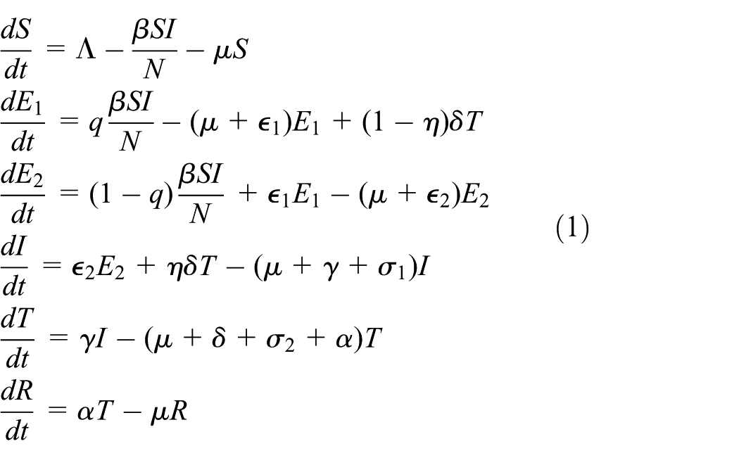
In this section, we construct the proposed TB transmission model with two latent classes in order to explore the slow and fast progression of the latent compartments. To develop the model we further divided the total population into six subclass: the susceptible $S(t)$ , slow and fast exposed classes are denoted by $E_1(t)$ and $E_2(t)$ respectively, TB infected $I(t)$ , treated $T(t)$ , and finally recovered individuals are expressed as $R(t)$ . We assume that after interaction with an infected individual, a suspectable person moves to either slow or fast latent class depending on the status of the infected individuals. Furthermore, we assume that the individuals in the slow exposed class must go through the fast class before moving the infected one. The flow of model dynamics among the different compartments is shown in Figure 1.

Figure 1.

Flowchart for the TB transmission model.

Based on these assumptions and the flow among different compartments depicted in Figure 1, the proposed TB model is governed by the following system of nonlinear differential equations

$$\begin{array}{c}\frac{\mathrm{dS}}{\mathrm{dt}}=\mathrm{\Lambda }-\frac{\beta \mathrm{SI}}{N}-\mu S\hfill \\ \frac{d{E}_1}{\mathrm{dt}}=q\frac{\beta \mathrm{SI}}{N}-(\mu +{ϵ}_1)E_1+(1-\eta )\delta T\hfill \\ \frac{d{E}_2}{\mathrm{dt}}=(1-q)\frac{\beta \mathrm{SI}}{N}+{ϵ}_1{E}_1-(\mu +{ϵ}_2)E_2\hfill \\ \frac{\mathrm{dI}}{\mathrm{dt}}={ϵ}_2{E}_2+\eta \delta T-(\mu +\gamma +{\sigma }_1)I\hfill \\ \frac{\mathrm{dT}}{\mathrm{dt}}=\gamma I-(\mu +\delta +{\sigma }_2+\alpha )T\hfill \\ \frac{\mathrm{dR}}{\mathrm{dt}}=\alpha T-\mu R\hfill \end{array}$$

(1)

subject to the nonnegative initial conditions

$$\begin{array}{c}S(0)>0,E_1(0)\ge 0,E_2(0)\ge 0,I(0)\ge 0,\hfill \\ T(0)\ge 0,R(0)\ge 0\hfill \end{array}$$

In the above system we have, $N(t)=S(t)+E_1(t)+E_2(t)+I(t)+T(t)+R(t).$

In model (1), after effective interaction with infected individuals, a fraction $q$ $(0<q<1)$ of $S(t)$ enter to slow exposed class $E_1$ and a fraction $1-q$ enter directly to the fast exposed class $E_2$ . The parameter $\mathrm{\Lambda }$ denotes is birth rate, $\beta$ is the successful transmission coefficient, $\mu$ is natural death rate in all classes, ${\sigma }_1$ and ${\sigma }_2$ are, respectively, the disease death rates in $I$ and $T$ compartments, ${ϵ}_1$ is the progression from compartment $E_1$ to $E_2$ , ${ϵ}_2$ denote the progression from compartment $E_2$ to $I$ and $\gamma$ expresses the per capita treatment rate of infected people. The people in the treated compartment leave the class with incomplete treatment at the rate $\delta$ and a fraction of which $(\eta \delta T)$ reenter to infected class $I$ while the rest $((1-\eta )\delta T)$ rejoin the slow expose class $E_1$ , depending upon the stage of their treatment. The parameter $\alpha$ represents the rate at which the treated individuals enter to recovery class. In the factor $(1-\eta )\delta$ , the parameter $\eta$ $(0<\eta <1)$ reflects the fraction of drug-resistance individuals in treated class.

To express model (1) in simple form, let us denote

$$\begin{array}{c}{k}_1=(\mu +{ϵ}_1),k_2=(\mu +{ϵ}_2),k_3=(\mu +\gamma +{\sigma }_1),\hfill \\ k_4=(\mu +\delta +{\sigma }_2+\alpha )\hfill \end{array}$$

Model (1) can be written as

$$\begin{array}{c}\frac{\mathrm{dS}}{\mathrm{dt}}=\mathrm{\Lambda }-\frac{\beta \mathrm{SI}}{N}-\mu S\hfill \\ \frac{d{E}_1}{\mathrm{dt}}=q\frac{\beta \mathrm{SI}}{N}-k_1{E}_1+(1-\eta )\delta T\hfill \\ \frac{d{E}_2}{\mathrm{dt}}=(1-q)\frac{\beta \mathrm{SI}}{N}+{ϵ}_1{E}_1-k_2{E}_2\hfill \\ \frac{\mathrm{dI}}{\mathrm{dt}}={ϵ}_2{E}_2+\eta \delta T-k_{3}I\hfill \\ \frac{\mathrm{dT}}{\mathrm{dt}}=\gamma I-k_{4}T\hfill \\ \frac{\mathrm{dR}}{\mathrm{dt}}=\alpha T-\mu R\hfill \end{array}$$

(2)

Parameter estimations

This part of the article aims to estimate the parameters associated to the TB disease model given by equation (2) in order to illustrate the numerical simulations. The actual TB incidence cases from 2002 to 2017 reported in Khyber Pakhtunkhwa obtained from the NTP ⁷ are used to estimate the parameter values. These are the TB infected cases conformed and tested positive using laboratory tests. In order to parameterize model (2), we adopt two approaches: two parameter values, $\mu$ and $\mathrm{\Lambda }$ , are obtained from the literature while the rest are fitted from the real TB statistics using least square curve fitting technique. The parameter estimation details are as follows: the natural death rate given by $\mu$ is obtained as the reciprocal of the average lifespan in Pakistan. The average lifespan in Pakistan is 67.7 years, ¹ therefore, $\mu =1/67.7$ per year. For the demographic parameter, $\mathrm{\Lambda }$ , the birth rate is calculated as follows: we consider the year 2017, and the population of Khyber Pakhtunkhwa according to the year 2017 is given as 30,523,371, ⁶ Further assuming $\mathrm{\Lambda }/\mu =30,523,371$ which is considered to be the limiting population in the absence of disease, therefore, $\mathrm{\Lambda }=450,862.20088626$ per year. The list of the remaining system parameters are obtained by using the curve fitting for the given incidence data using the least-square curve fitting in MATLAB. In Figure 2, it is shown that the model solution is in good agreement with the field data. The basic steps in the parameter estimation procedure are summarized as follows. Model (2) can be expressed as

$$\frac{\mathrm{dy}}{\mathrm{dt}}=\mathcal{F}(t,y,\mathrm{\Theta }),y(t_0)=y_0$$

(3)

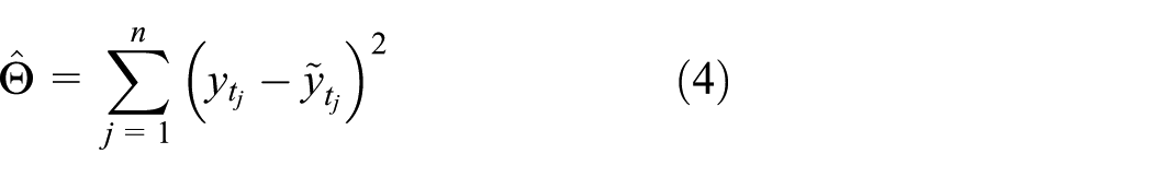
where $y$ and $\mathrm{\Theta }$ are the vectors of dependent variables and unknown parameters, respectively. One can have the best set of parameter values of reducing the error among the TB cases and the model solution. In this process, the following objective function is considered and is given as

$$\hat{\mathrm{\Theta }}=\sum _{j=1}^n{(y_{t_j}-{\tilde{y}}_{t_j})}^2$$

(4)

where ${\tilde{y}}_{t_j}$ are the actual cases and $y_{t_j}$ denotes the solution of the model at time $t_j,$ and $n$ denotes the available actual data points. To obtain the model parameters, the aim is to minimize the following objective function

$$\{\begin{array}{c}\min \hat{\mathrm{\Theta }}\hfill \\ \multicolumn{1}{c}{\mathrm{subject}\mathrm{to}\mathrm{Eq}.(3)}\end{array}$$

(5)

The parameter estimation algorithm can be summarized in the following steps:

1. Choose initial parameter values and state variables.

2. Solve model (3) numerically using Runge–Kutta order four (RK4) method with initial data chosen in step (1).

3. Evaluate error using the expression in equation (4).

4. Using an optimization algorithm presented in Kristensen, ¹⁵ minimize (5) and obtain a new set of parameter values with the model outcomes in order to get better agreement with the real data.

5. Confirm the convergence criteria. If not converged, go to step (2) again.

6. This iteration process between parameter updating and numerical solutions of the system will continue till the desired convergence criteria for the parameters are obtained.

Using the above algorithm, we obtained the fitted values of the parameters for model (2), which are tabulated in Table 1. A comparison of the actual cases of TB incidence and the model simulation is shown in Figure 2, where the actual cases are shown graphically by circles whereas the model simulation is shown by a bold line. Consequently, using these parameters, the value of ${\mathcal{R}}_0$ associated to the TB disease model given by equation (2) for Khyber Pakhtunkhwa is approximately 1.38.

Table 1.

Fitted or estimated values of parameters for model (2).

Parameter	Details	Baseline value	Source
$\mathrm{\Lambda }$	Birth rate	450,862.20088	Estimated
$\beta$	Contact rate	0.6001	Fitted
$\alpha$	Recovery rate	0.0100	Fitted
$\gamma$	Treatment rate of infective individuals	0.1500	Fitted
$\mu$	Natural mortality rate	1/67.7	Pakistan Bureau of Statistics 5
${\sigma }_1$	Disease induced death rate in $I$	0.2738	Fitted
${\sigma }_2$	Disease induced death rate during treatment	0.1000	Fitted
$\delta$	Leaving rate of treated individual re-enter to $I$ or $E_1$	0.0649	Fitted
$\eta$	Failure of treatment	0.2959	Fitted
${ϵ}_1$	Rate of moving from $E_1$ to $E_2$	0.2351	Fitted
${ϵ}_2$	Transfer rate from $E_2$ to $I$	0.2001	Fitted
$q$	Fraction of susceptible individuals being infected	0.5259	Fitted

Figure 2.

Model solution versus data.

Model analysis

Here, some of the important basic mathematical results associated with the TB disease system given by equation (2) are analyzed. Initially, we prove the positivity and solution boundedness.

Boundedness and positivity

In order to ensure that the TB infection model described in equation (2) is meaningful from the epidemiological point of view, it is necessary to prove that the solutions of system (2) with nonnegative initial conditions will remain nonnegative for any value of $t$ such that $t>0$ . For this purpose we present the following lemma.

Lemma 1

For the initial information $\mathcal{H}(0)\ge 0$ , where $\mathcal{H}(t)=(S(t),E_1(t),E_2,I(t),T(t),R(t))$ , the solutions of system (2) will be nonnegative whenever they exist.

Proof

Suppose $\phi (t)=\beta I/N$ and $\mathcal{I}\subset [0,\infty )$ , then the first equation of system (2) yields

$$\frac{\mathrm{dS}}{\mathrm{dt}}=\mathrm{\Lambda }-(\phi (t)+\mu )S$$

(6)

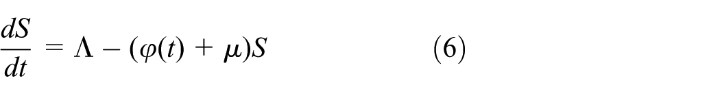
Under the considered assumption, a solution for the TB disease model shown in equation (2) exists in $\mathcal{I}$ , then the corresponding solution of equation (6) can be obtained as follows

$$\begin{array}{c}S(t)=S(0)\exp \hfill \\ \{-(\mu t+\underset{0}{\overset{t}{\int }}\phi (u)\mathrm{du})\}+\exp \{-(\mu t+\underset{0}{\overset{t}{\int }}\phi (u)\mathrm{du})\}\hfill \\ \times \underset{0}{\overset{t}{\int }}\mathrm{\Lambda }\exp \{\mu x+\underset{0}{\overset{x}{\int }}\phi (z)\mathrm{dz}\}\mathrm{dx}>0\hfill \end{array}$$

Similarly, we can show for the rest of the variables in $\mathcal{H}$ , that is, $\mathcal{H}>0$ , $\forall t>0$ .   □

Invariant region

The dynamics of the TB transmission system shown in equation (2) having a feasible region that is biologically meaningfulis given as

$$\mathrm{\Phi }\subset {\mathbb{R}}_{+}^6$$

where

$$\mathrm{\Phi }=\{(S(t),E_1(t),E_2(t),I(t),T(t),R(t))\in {\mathbb{R}}_{+}^6:S(t)+E_1(t)+E_2(t)+I(t)+T(t)+R(t)\le \mathrm{\Lambda }/\mu \}$$

Lemma 2

The region shown by $\mathrm{\Phi }\subset {\mathbb{R}}_{+}^6$ , for the TB disease given in equation (2) is positive invariant with the nonnegative initial conditions in ${\mathbb{R}}_{+}^6$ .

Proof

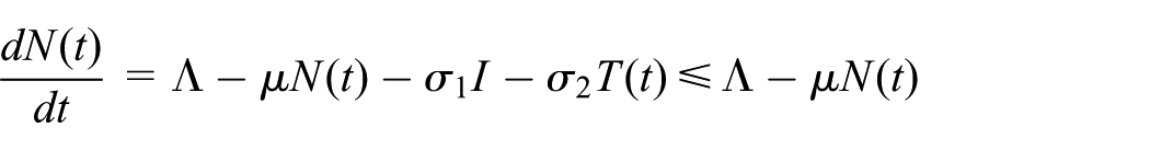
From the addition of all equations of model (2), we obtained

$$\frac{\mathrm{dN}(t)}{\mathrm{dt}}=\mathrm{\Lambda }-\mu N(t)-{\sigma }_{1}I-{\sigma }_{2}T(t)\le \mathrm{\Lambda }-\mu N(t)$$

Clearly

$$\frac{\mathrm{dN}(t)}{\mathrm{dt}}\le 0,\mathrm{if}N(t)\ge \mathrm{\Lambda }/\mu$$

Hence

$$N(t)\le N(0)e^{-\mu t}+\frac{\mathrm{\Lambda }}{\mu }(1-e^{-\mu t})$$

Therefore, $N(t)\le \mathrm{\Lambda }/\mu$ if $N(0)\le \mathrm{\Lambda }/\mu$ . On the other hand, if $N(0)>\mathrm{\Lambda }/\mu$ , then $N(t)\to \mathrm{\Lambda }/\mu$ , as $t\to \infty$ . Thus, the region $\mathrm{\Phi }$ is positively invariant and attracts all solutions in ${\mathbb{R}}_{+}^6$ .

Basic reproduction number and equilibria

Model (2) has a disease-free equilibrium (DFE), ${\mathcal{D}}_0$ , given as

$${\mathcal{D}}_0=(\frac{\mathrm{\Lambda }}{\mu },0,0,0,0,0)$$

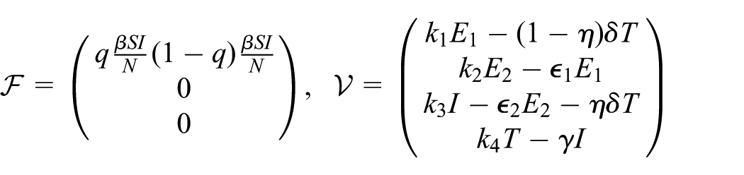
The qualitative dynamics of such models are completely examined by a threshold parameter, known as the basic reproduction number and is usually denoted by $R_0$ . This important threshold quantity is defined as “an average number of tuberculosis infections is inserted to purely susceptible population that generate further secondary infection cases of tuberculosis by a typical infected person.” ¹⁶ With the help of ${\mathcal{R}}_0$ one can determine that either the infectious disease will remain or die out in a population. If ${\mathcal{R}}_0<1$ , then it means that one infected person on average can infect less than one person and, therefore, the disease will die out in time. If ${\mathcal{R}}_0>1$ , then it means that one infected individual will infect more than one susceptible individuals on average and, hence, the disease will persist in the population. The basic reproduction number for a disease model is usually determined by the well-known next-generation method presented in Van den Driessche and Watmough. ¹⁶ The corresponding matrices to compute $R_0$ are given as

$$\mathcal{F}=\left(\begin{array}{c}q\frac{\beta \mathrm{SI}}{N}(1-q)\frac{\beta \mathrm{SI}}{N}\hfill \\ \multicolumn{1}{c}{0}\\ \multicolumn{1}{c}{0}\end{array}\right),\mathcal{V}=\left(\begin{array}{c}{k}_1{E}_1-(1-\eta )\delta T\hfill \\ \multicolumn{1}{c}{k_2{E}_2-{ϵ}_1{E}_1}\\ \multicolumn{1}{c}{k_{3}I-{ϵ}_2{E}_2-\eta \delta T}\\ \multicolumn{1}{c}{k_{4}T-\gamma I}\end{array}\right)$$

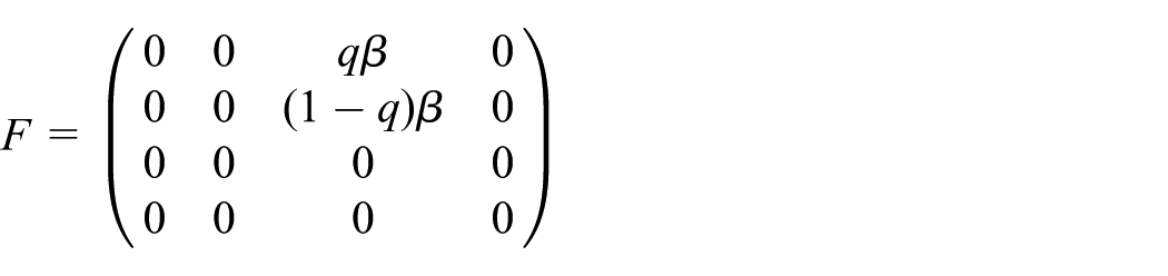
The Jacobian of the above matrices are given as

$$F=\left(\begin{array}{cccc}0\hfill & 0\hfill & q\beta \hfill & 0\hfill \\ \multicolumn{1}{c}{0}& 0\hfill & (1-q)\beta \hfill & 0\hfill \\ \multicolumn{1}{c}{0}& 0\hfill & 0\hfill & 0\hfill \\ \multicolumn{1}{c}{0}& 0\hfill & 0\hfill & 0\hfill \end{array}\right)$$

$$V=\left(\begin{array}{cccc}{k}_1\hfill & 0\hfill & 0\hfill & -\delta (1-\eta )\hfill \\ \multicolumn{1}{c}{-{ϵ}_1}& k_2\hfill & 0\hfill & 0\hfill \\ \multicolumn{1}{c}{0}& -{ϵ}_2\hfill & k_3\hfill & -\delta \eta \hfill \\ \multicolumn{1}{c}{0}& 0\hfill & -\gamma \hfill & k_4\hfill \end{array}\right)$$

Hence, using ${\mathcal{R}}_0=\rho (F{V}^{-1})$ , where $\rho (.)$ denotes the spectral radius, the basic reproduction number is obtained as

$$R_0=\frac{\beta k_4{ϵ}_2(q{ϵ}_1+(1-q)k_1)}{k_1{k}_2(k_3{k}_4-\gamma \delta \eta )-{ϵ}_1{ϵ}_2\gamma \delta (1-\eta )}$$

Following (Theorem 2), ¹⁶ we present the below theorem to show that model (2) is locally asymptotically stable (LAS) of DFE ${\mathcal{D}}_0$ .

Theorem 1

The DFE ${\mathcal{D}}_0$ of the TB transmission model is LAS if and only if $R_0<1$ .

Proof

To prove LAS, we need to verify the hypothesis, namely, $(A_1)-(A_5)$ given in Van den Driessche and Watmough. ¹⁶ The hypothesis $(A_1)-(A_4)$ is easy to verify. To verify $A_5$ it is enough to prove that each eigenvalue associated to $J_{{\mathcal{D}}_0}$ has negative real parts

$$J_{{\mathcal{D}}_0}=\left(\begin{array}{cc}\mathcal{M}\hfill & 0\hfill \\ \multicolumn{1}{c}{J_3}& J_4\hfill \end{array}\right)$$

where

$$\begin{array}{c}\multicolumn{1}{c}{J_3=-F,\mathcal{M}=F-V}\\ =\left(\begin{array}{cccc}-k_1\hfill & 0\hfill & q\beta \hfill & (1-\eta )\delta \hfill \\ \multicolumn{1}{c}{{ϵ}_1}& -k_2\hfill & (1-q)\beta \hfill & 0\hfill \\ \multicolumn{1}{c}{0}& {ϵ}_2\hfill & -k_3\hfill & \eta \delta \hfill \\ \multicolumn{1}{c}{0}& 0\hfill & \gamma \hfill & -k_4\hfill \end{array}\right)\hfill \end{array}$$

and

$$J_4=\left(\begin{array}{cccc}-k_1\hfill & 0\hfill & 0\hfill & (1-\eta )\delta \hfill \\ \multicolumn{1}{c}{{ϵ}_1}& -k_2\hfill & 0\hfill & 0\hfill \\ \multicolumn{1}{c}{0}& {ϵ}_2\hfill & -k_3\hfill & \eta \delta \hfill \\ \multicolumn{1}{c}{0}& 0\hfill & \gamma \hfill & -k_4\hfill \end{array}\right)$$

Define $s(\mathcal{M})=\max \{\mathrm{Re}\lambda :\lambda \mathrm{is}\mathrm{an}\mathrm{eigenvalue}\mathrm{of}\mathcal{M}\}$ , where $s(\mathcal{M})$ is the simple eigenvalue of matrix $\mathcal{M}$ with a positive eigenvector, then from, ¹⁶ we have, $R_0<1$ $\iff s(\mathcal{M})<0.$ Also, calculating eigenvalues associated with $J_4$ , we have

$$s(J_4)=\max (-k_1,-k_2,-k_3,-k_4)<0$$

Hence, if $R_0<1$ , then $s(J_{{\mathcal{D}}_0})<0$ , the point ${\mathcal{D}}_0$ is LAS.

Lemma 3

If $R_0>1$ then the TB disease model possesses a unique endemic equilibrium (EE) which is positive.

Proof

The EE of equation (2) denoted by ${\mathcal{D}}_1=(S^{*},E_1^{*},E_2^{*},I^{*},T^{*},R^{*})$ , is derived by setting equal to zero the right-hand side of model (2). After simplification, we obtained the following expressions for EE as

$$\{\begin{array}{c}{S}^{*}=\frac{N^{*}}{R_0}\hfill \\ E_1^{*}=\frac{1}{k_1{k}_4}(\frac{k_{4}q\beta }{R_0}+(1-\eta )\gamma \delta )I^{*}\hfill \\ E_2^{*}=\frac{1}{{ϵ}_2{k}_4}(k_4{k}_3-\eta \gamma \delta )I^{*}\hfill \\ T^{*}=\frac{\gamma }{k_4}{I}^{*}\hfill \\ R^{*}=\frac{\alpha \gamma }{\mu k_4}{I}^{*}\hfill \\ I^{*}=\frac{k_1{k}_4\mu {ϵ}_2(R_0-1)N^{*}}{k_4\mu {ϵ}_{2}q\beta +(\mu (k_1(k_3{k}_4-\eta \gamma \delta )+\gamma {ϵ}_2(k_1+(1-\eta )\delta ))+k_1{ϵ}_2(\alpha \gamma +k_4\mu ))R_0}\hfill \end{array}$$

It is clear from the above expressions that a unique EE exists whenever $R_0>1$ .

Global stability analysis

In this section, we explore the global stability results for both DFE and EE of the model. We proceed with the following theorem.

Theorem 2

For $R_0<1$ , the DFE ${\mathcal{D}}_0$ of model (2) is globally asymptotically stable (GAS) on $\mathrm{\Phi }$ and unstable for 1.

Proof

Let us define the following Lyapunov function in order to prove GAS

$$\mathcal{L}(t)={\mathcal{C}}_1{E}_1+{\mathcal{C}}_2{E}_2+{\mathcal{C}}_{3}I+{\mathcal{C}}_{4}T$$

where ${\mathcal{C}}_i>0$ , with $i=1,...,4$ , which is to be obtained later. Time differentiation of $\mathcal{L}(t)$ and use of the model described by equation (2), the following is presented

$$\begin{array}{c}\multicolumn{1}{c}{\frac{d\mathcal{L}(t)}{\mathrm{dt}}={\mathcal{C}}_1\{q\frac{\beta \mathrm{SI}}{N}-k_1{E}_1+(1-\eta )\delta T\}}\\ +{\mathcal{C}}_2\{(1-q)\frac{\beta \mathrm{SI}}{N}+{ϵ}_1{E}_1-k_2{E}_2\}+\hfill \\ {\mathcal{C}}_3\{{ϵ}_2{E}_2+\eta \delta T-k_{3}I\}+{\mathcal{C}}_4\{\gamma I-k_{4}T\}\hfill \\ \le {\mathcal{C}}_1\{q\beta I-k_1{E}_1+(1-\eta )\delta T\}\hfill \\ +{\mathcal{C}}_2\{(1-q)\beta I+{ϵ}_1{E}_1-k_2{E}_2\}+\hfill \\ {\mathcal{C}}_3\{{ϵ}_2{E}_2+\eta \delta T-k_{3}I\}+{\mathcal{C}}_4\{\gamma I-k_{4}T\},S\le N\hfill \\ =\{{\mathcal{C}}_{1}q\beta +{\mathcal{C}}_2(1-q)\beta +{\mathcal{C}}_4\gamma -{\mathcal{C}}_3{k}_3\}I\hfill \\ +\{{\mathcal{C}}_2{ϵ}_1-{\mathcal{C}}_1{k}_1\}{E}_1+\{{\mathcal{C}}_3{ϵ}_2-{\mathcal{C}}_2{k}_2\}{E}_2\hfill \\ +\{{\mathcal{C}}_1(1-\eta )\delta +{\mathcal{C}}_3\eta \delta -{\mathcal{C}}_4{k}_4\}T\hfill \\ \le {\mathcal{C}}_3{k}_3\{\frac{{\mathcal{C}}_{1}q\beta +{\mathcal{C}}_2(1-q)\beta +{\mathcal{C}}_4\gamma }{{\mathcal{C}}_3{k}_3}-1\}I\hfill \\ +\{{\mathcal{C}}_2{ϵ}_1-{\mathcal{C}}_1{k}_1\}{E}_1+\{{\mathcal{C}}_3{ϵ}_2-{\mathcal{C}}_2{k}_2\}{E}_2\hfill \\ +\{{\mathcal{C}}_1(1-\eta )\delta +{\mathcal{C}}_3\eta \delta -{\mathcal{C}}_4{k}_4\}T\hfill \end{array}$$

Now choosing

$$\begin{array}{c}{\mathcal{C}}_1={ϵ}_1,{\mathcal{C}}_2=k_1,{\mathcal{C}}_3=\frac{k_1{k}_2}{{ϵ}_2}\mathrm{and}\hfill \\ {\mathcal{C}}_4=\frac{{ϵ}_1{ϵ}_2(1-\eta )\delta +k_1{k}_2\eta \delta }{{ϵ}_2{k}_4}\hfill \end{array}$$

further simplification gives

$$\frac{d\mathcal{L}(t)}{\mathrm{dt}}\le {\mathcal{C}}_3{k}_3(R_0-1)I$$

(7)

Hence, if $R_0<1$ then $d\mathcal{L}(t)/\mathrm{dt}<0$ . Therefore, the largest compact invariant set in $\mathrm{\Phi }$ is the singleton set ${\mathcal{D}}_0$ and thus by LaSalle’s invariant principle ¹⁷ the DFE ${\mathcal{D}}_0$ is GAS in $\mathrm{\Phi }$ .

Next, we provide the result for GAS of the TB disease model shown by equation (2) at EE ${\mathcal{D}}_1$ . We obtain the following relations from equation (2) at EE as

$$\{\begin{array}{c}\mathrm{\Lambda }=\frac{\beta S^{*}{I}^{*}}{N^{*}}+\mu S^{*}\hfill \\ k_1{E}_1^{*}=\frac{q\beta S^{*}{I}^{*}}{N^{*}}+(1-\eta )\delta T^{*}\hfill \\ k_2{E}_2^{*}=\frac{(1-q)\beta S^{*}{I}^{*}}{N^{*}}+{ϵ}_1{E}_1^{*}\hfill \\ k_3{I}^{*}={ϵ}_2{E}_2^{*}+\eta \delta T^{*}\hfill \\ \gamma I^{*}=k_4{T}^{*}\hfill \end{array}$$

(8)

Furthermore, we state the following theorem.

Theorem 3

The EE of the model (2) is GAS, if $R_0>1$ .

Proof

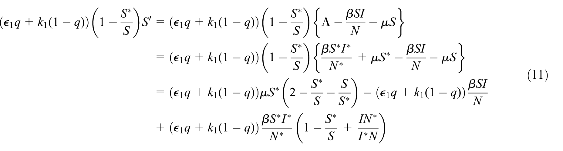
The following Lyapunov function is considered to show the result

$$\begin{array}{c}\multicolumn{1}{c}{\mathcal{K}(t)=({ϵ}_{1}q+k_1(1-q))\{S(t)-S^{*}-S^{*}\ln \frac{S(t)}{S^{*}}\}}\\ +{ϵ}_1\{E_1(t)-E_1^{*}-E_1^{*}\ln \frac{E_1(t)}{E_1^{*}}\}\hfill \\ +k_1\{E_2(t)-E_2^{*}-E_2^{*}\ln \frac{E_2(t)}{E_2^{*}}\}\hfill \\ +\frac{k_1{k}_2}{{ϵ}_2}\{I(t)-I^{*}-I^{*}\ln \frac{I(t)}{I^{*}}\}\hfill \\ +\frac{\delta T^{*}({ϵ}_1{ϵ}_2\eta +k_1{k}_2(1-\eta ))}{\gamma {ϵ}_2{I}^{*}}\hfill \\ \{T(t)-T^{*}-T^{*}\ln \frac{T(t)}{T^{*}}\}\hfill \end{array}$$

(9)

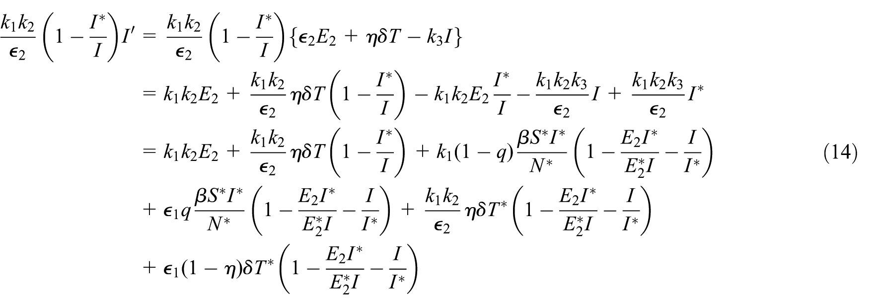
The differentiation of equation (9) with use of the model equations, the following is obtained

$$\begin{array}{c}\multicolumn{1}{c}{\frac{d\mathcal{K}(t)}{\mathrm{dt}}=({ϵ}_{1}q+k_1(1-q))(1-\frac{S^{*}}{S})S\prime }\\ +{ϵ}_1(1-\frac{E_1^{*}}{E_1})E{\prime }_1+k_1(1-\frac{E_2^{*}}{E_2})E{\prime }_2\hfill \\ +\frac{k_1{k}_2}{{ϵ}_2}(1-\frac{I^{*}}{I})I\prime \hfill \\ +\frac{\delta T^{*}({ϵ}_1{ϵ}_2\eta +k_1{k}_2(1-\eta ))}{\gamma {ϵ}_2{I}^{*}}(1-\frac{T^{*}}{T})T\prime \hfill \end{array}$$

(10)

It follows from equation (8) and direct calculation shows that

$$\begin{array}{c}\multicolumn{1}{c}{({ϵ}_{1}q+k_1(1-q))(1-\frac{S^{*}}{S})S\prime =({ϵ}_{1}q+k_1(1-q))(1-\frac{S^{*}}{S})\{\mathrm{\Lambda }-\frac{\beta \mathrm{SI}}{N}-\mu S\}}\\ =({ϵ}_{1}q+k_1(1-q))(1-\frac{S^{*}}{S})\{\frac{\beta S^{*}{I}^{*}}{N^{*}}+\mu S^{*}-\frac{\beta \mathrm{SI}}{N}-\mu S\}\hfill \\ =({ϵ}_{1}q+k_1(1-q))\mu S^{*}(2-\frac{S^{*}}{S}-\frac{S}{S^{*}})-({ϵ}_{1}q+k_1(1-q))\frac{\beta \mathrm{SI}}{N}\hfill \\ +({ϵ}_{1}q+k_1(1-q))\frac{\beta S^{*}{I}^{*}}{N^{*}}(1-\frac{S^{*}}{S}+\frac{I{N}^{*}}{I^{*}N})\hfill \end{array}$$

(11)

$$\begin{array}{c}\multicolumn{1}{c}{{ϵ}_1(1-\frac{E_1^{*}}{E_1})E{\prime }_1={ϵ}_1(1-\frac{E_1^{*}}{E_1})\{q\frac{\beta \mathrm{SI}}{N}-k_1{E}_1+(1-\eta )\delta T\}}\\ ={ϵ}_{1}q\frac{\beta \mathrm{SI}}{N}(1-\frac{E_1^{*}}{E_1})+{ϵ}_1(1-\eta )\delta T(1-\frac{E_1^{*}}{E_1})-k_1{ϵ}_1{E}_1+k_1ϵE_1^{*}\hfill \\ ={ϵ}_{1}q\frac{\beta \mathrm{SI}}{N}(1-\frac{E_1^{*}}{E_1})+{ϵ}_1(1-\eta )\delta T(1-\frac{E_1^{*}}{E_1})-k_1{ϵ}_1{E}_1+{ϵ}_{1}q\frac{\beta S^{*}{I}^{*}}{N^{*}}\hfill \\ +{ϵ}_1(1-\eta )\delta T^{*}\hfill \end{array}$$

(12)

$$\begin{array}{c}{k}_1(1-\frac{E_2^{*}}{E_2})E{\prime }_2=k_1(1-\frac{E_2^{*}}{E_2})\{(1-q)\frac{\beta \mathrm{SI}}{N}+{ϵ}_1{E}_1-k_2{E}_2\}\hfill \\ =k_1(1-q)\frac{\beta \mathrm{SI}}{N}(1-\frac{E_2^{*}}{E_2})+k_1{ϵ}_1{E}_1-k_1{ϵ}_1{E}_1\frac{E_2^{*}}{E_2}-k_1{k}_2{E}_2+k_1{k}_2{E}_2^{*}\hfill \\ =k_1(1-q)\frac{\beta \mathrm{SI}}{N}(1-\frac{E_2^{*}}{E_2})+k_1{ϵ}_1{E}_1-k_1{k}_2{E}_2+{ϵ}_{1}q\frac{\beta S^{*}{I}^{*}}{N^{*}}(1-\frac{E_1{E}_2^{*}}{E_1^{*}{E}_2})\hfill \\ +{ϵ}_1(1-\eta )\delta T^{*}(1-\frac{E_1{E}_2^{*}}{E_1^{*}{E}_2})\hfill \end{array}$$

(13)

$$\begin{array}{c}\multicolumn{1}{c}{\frac{k_1{k}_2}{{ϵ}_2}(1-\frac{I^{*}}{I})I\prime =\frac{k_1{k}_2}{{ϵ}_2}(1-\frac{I^{*}}{I})\{{ϵ}_2{E}_2+\eta \delta T-k_{3}I\}}\\ =k_1{k}_2{E}_2+\frac{k_1{k}_2}{{ϵ}_2}\eta \delta T(1-\frac{I^{*}}{I})-k_1{k}_2{E}_2\frac{I^{*}}{I}-\frac{k_1{k}_2{k}_3}{{ϵ}_2}I+\frac{k_1{k}_2{k}_3}{{ϵ}_2}{I}^{*}\hfill \\ =k_1{k}_2{E}_2+\frac{k_1{k}_2}{{ϵ}_2}\eta \delta T(1-\frac{I^{*}}{I})+k_1(1-q)\frac{\beta S^{*}{I}^{*}}{N^{*}}(1-\frac{E_2{I}^{*}}{E_2^{*}I}-\frac{I}{I^{*}})\hfill \\ +{ϵ}_{1}q\frac{\beta S^{*}{I}^{*}}{N^{*}}(1-\frac{E_2{I}^{*}}{E_2^{*}I}-\frac{I}{I^{*}})+\frac{k_1{k}_2}{{ϵ}_2}\eta \delta T^{*}(1-\frac{E_2{I}^{*}}{E_2^{*}I}-\frac{I}{I^{*}})\hfill \\ +{ϵ}_1(1-\eta )\delta T^{*}(1-\frac{E_2{I}^{*}}{E_2^{*}I}-\frac{I}{I^{*}})\hfill \end{array}$$

(14)

$$\begin{array}{c}\frac{\delta T^{*}({ϵ}_1{ϵ}_2(1-\eta )+k_1{k}_2\eta )}{{ϵ}_2\gamma I^{*}}(1-\frac{T^{*}}{T})\{\gamma I-k_{3}T\}=\delta T^{*}({ϵ}_1(1-\eta )+\frac{k_1{k}_2\eta }{{ϵ}_2})\hfill \\ \times (1+\frac{I}{I^{*}}-\frac{I{T}^{*}}{I^{*}T}-\frac{T}{T^{*}})\hfill \end{array}$$

(15)

Putting relations equations (11)–(15) into equation (10) and after simplification, we get

$$\begin{array}{c}\frac{d\mathcal{K}(t)}{\mathrm{dt}}=\mu ({ϵ}_{1}q+k_1(1-q))S^{*}(2-\frac{S^{*}}{S}-\frac{S}{S^{*}})+\frac{k_1{k}_2}{{ϵ}_2}\eta \delta T^{*}(2-\frac{T}{T^{*}}-\frac{I{T}^{*}}{I^{*}T})\hfill \\ +{ϵ}_1(1-\eta )\delta T^{*}(4-\frac{E_1^{*}T}{E_1{T}^{*}}-\frac{E_1{E}_2^{*}}{E_1^{*}{E}_2}-\frac{I^{*}{E}_2}{{\mathrm{IE}}_2^{*}}-\frac{I{T}^{*}}{I^{*}T})\hfill \\ q{ϵ}_1\frac{\beta S^{*}{I}^{*}}{N^{*}}(4-\frac{S^{*}}{S}-\frac{I}{I^{*}}-\frac{E_1{E}_2^{*}}{E_1^{*}{E}_2}-\frac{E_2{I}^{*}}{E_2^{*}I}+\frac{I{N}^{*}}{I^{*}N}(1-\frac{\mathrm{IS}}{I^{*}{S}^{*}}))\hfill \\ k_1(1-q)\frac{\beta S^{*}{I}^{*}}{N^{*}}(3-\frac{S^{*}}{S}-\frac{I^{*}}{I}-\frac{E_2{I}^{*}}{E_2^{*}I}+\frac{I{N}^{*}}{I^{*}N}(1-\frac{{\mathrm{SE}}_2^{*}}{S^{*}{E}_2}))\hfill \end{array}$$

(16)

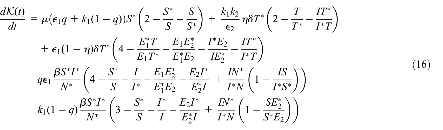
Using the arithmetical geometrical inequality, we have the following interpretation from equation (16)

$$\{\begin{array}{c}(2-\frac{S}{S^{*}}-\frac{S^{*}}{S})\le 0\hfill \\ (2-\frac{T}{T^{*}}-\frac{I{T}^{*}}{I^{*}T})\le 0\hfill \\ (4-\frac{E_1^{*}T}{E_1{T}^{*}}-\frac{E_1{E}_2^{*}}{E_1^{*}{E}_2}-\frac{I^{*}{E}_2}{{\mathrm{IE}}_2^{*}}-\frac{I{T}^{*}}{I^{*}T})\le 0\hfill \\ (4-\frac{S^{*}}{S}-\frac{I}{I^{*}}-\frac{E_1{E}_2^{*}}{E_1^{*}{E}_2}-\frac{E_2{I}^{*}}{E_2^{*}I}+\frac{I{N}^{*}}{I^{*}N}(1-\frac{\mathrm{IS}}{I^{*}{S}^{*}}))\le 0\hfill \\ (3-\frac{I^{*}}{I}-\frac{S^{*}}{S}-\frac{E_2{I}^{*}}{E_2^{*}I}+\frac{I{N}^{*}}{I^{*}N}(1-\frac{{\mathrm{SE}}_2^{*}}{S^{*}{E}_2}))\le 0\hfill \end{array}$$

(17)

Since the model parameters are nonnegative, following equation (17), we have $\frac{d\mathcal{K}(t)}{\mathrm{dt}}\le 0$ . Thus, if $R_0>1$ , then the LaSalle’s invariance principle ¹⁷ implies that $(S,E_1,E_2,I,T,R)\to (S^{*},E_1^{*},E_2^{*},I^{*},T^{*},R^{*})$ as $t\to \infty$ .

Model sensitivity

The sensitivity analysis of $R_0$ versus the model parameters plays an important role in order to determine how best to reduce human mortality and morbidity. In this section, we carried out the sensitivity analysis of various model parameters in order to determine their relative importance to the basic reproduction number. We evaluate the partial derivatives of $R_0$ with respect to model parameters and used the parameter values given in Table 1. In order to calculate the sensitivity indices we use the following formula developed in Chitnis et al. ¹⁸

Definition 1

The normalized sensitivity index of $R_0$ depending on the differentiability on a parameter $\varpi$ is defined as follows

$$S_{\varpi }^{R_0}=\frac{\varpi }{R_0}\frac{\partial R_0}{\partial \varpi }$$

(18)

These indices along with signs are given in Table 2 which provide information that how crucial each parameter is to disease transmission and prevalence. A positive (+) sign in Table 2 indicates that the basic reproduction number $R_0$ will increase as the parameter increases. On the other hand, an index with negative (−) means that $R_0$ will decrease as the parameter is increased.

Table 2.

Sensitivity indices of $R_0$ to parameters of TB model.

Parameter	Sensitivity
$\beta$	1
$\alpha$	−0.00630597
$\gamma$	−0.263321
$\delta$	+0.0786803
$\eta$	+0.00853032
${ϵ}_1$	+0.0349677
${ϵ}_2$	+0.0743007
$\mu$	−0.137818
${\sigma }_1$	−0.69897
${\sigma }_2$	−0.0630597
$q$	−0.0320859

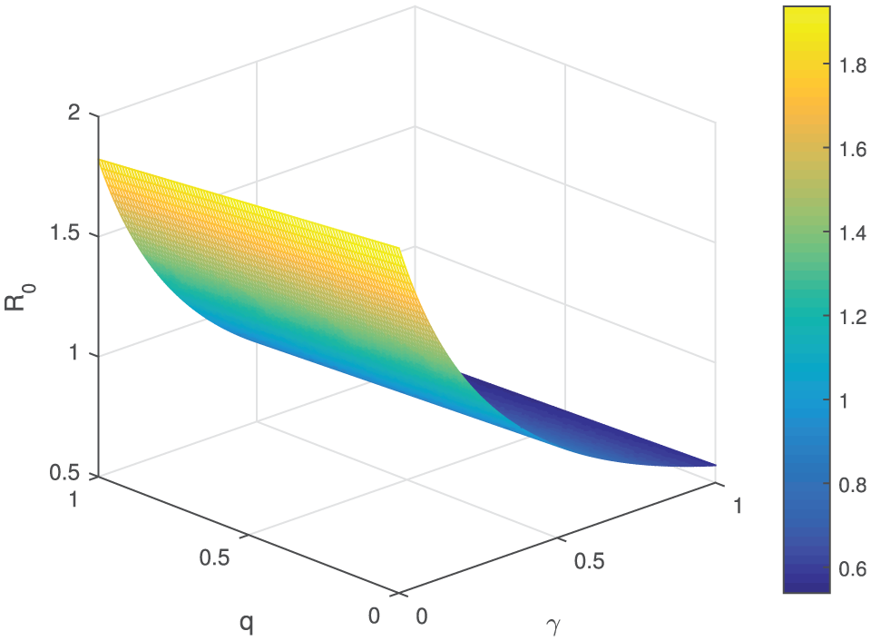
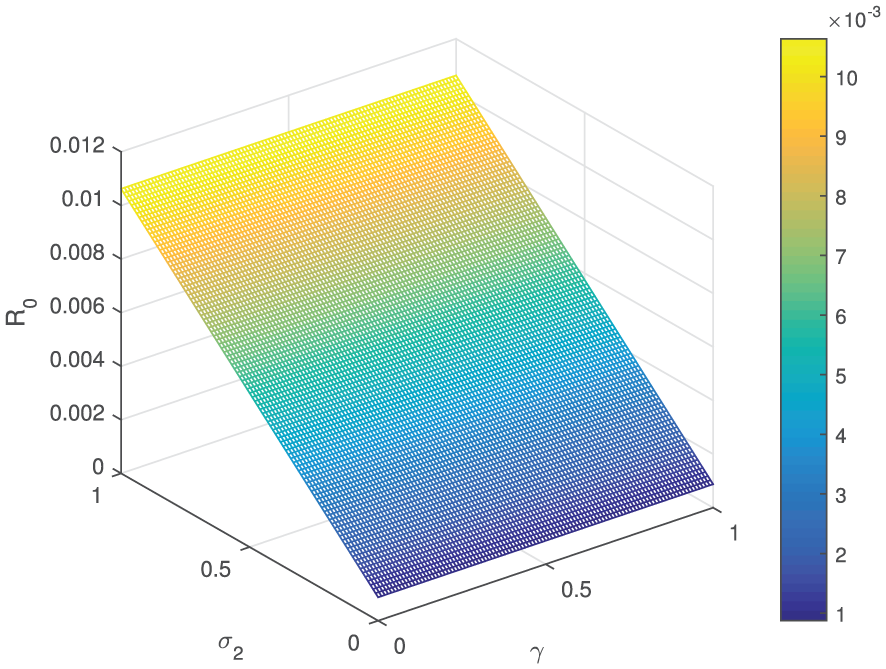
In Table 2, the parameters $\beta$ , $\delta$ , $\eta$ , ${ϵ}_1$ and ${ϵ}_2$ have indices with a positive sign. It means that these parameters have a direct effect on $R_0$ , that is, with the increase or decrease of these parameters, the value of $R_0$ will increase or decrease. This further means that with increase (or decrease) of the suggested parameters upto 10%, it will increase or decrease the value of $R_0$ by 10%, 0.7868%, 0.08530%, 0.349%, and 0.743%, respectively. The rest of the parameters $\alpha$ , $\gamma$ , $\mu$ , ${\sigma }_1$ , ${\sigma }_2$ and $q$ with negative indices have an inverse effect on $R_0$ , which means that increasing (or decreasing) of these rates by 10% will decrease (or increase) the basic reproduction number by 0.063%, 2.633 %, 1.378%, 6.989%, 0.630%, and 0.320%, respectively. The effect of different important model parameters on the value of $R_0$ is shown graphically in Figures 3–7. From Figure 3 we observe that $R_0$ is increasing with increased value of effective contact rate $\beta$ and the smaller value treatment rate $\gamma$ . A similar interpretation can be seen in Figure 4 for $\beta$ and ${\sigma }_1$ . Figure 5 depicts the effect of parameters $\beta$ and $\eta$ on $R_0$ . It is observed that $R_0$ increases significantly with these parameters and the maximum value of $R_0$ is close to 2.5, which means that epidemic will spread. Figures 6–8 show the variation in the value of $R_0$ for the increasing values of $\gamma$ and other parameters $q$ , ${ϵ}_1$ , and ${\sigma }_2$ , respectively. These figures reveal that the higher value of treatment rate $\gamma$ could decrease the value of the basic reproduction number $R_0$ and could be helpful to decrease elimination.

Figure 3.

Behavior of $R_0$ versus the parameters $\beta$ and $\gamma$ .

Figure 4.

Behavior of $R_0$ versus the parameters $\beta$ and ${\sigma }_1$ .

Figure 5.

Behavior of $R_0$ versus the parameters $\beta$ and $\eta$ .

Figure 6.

Behavior of $R_0$ versus the parameters $\gamma$ and $q$ .

Figure 7.

Behavior of $R_0$ versus the parameters $\gamma$ and ${ϵ}_1$ .

Figure 8.

Behavior of $R_0$ versus the parameters $\gamma$ and ${\sigma }_2$ .

Numerical results and discussion

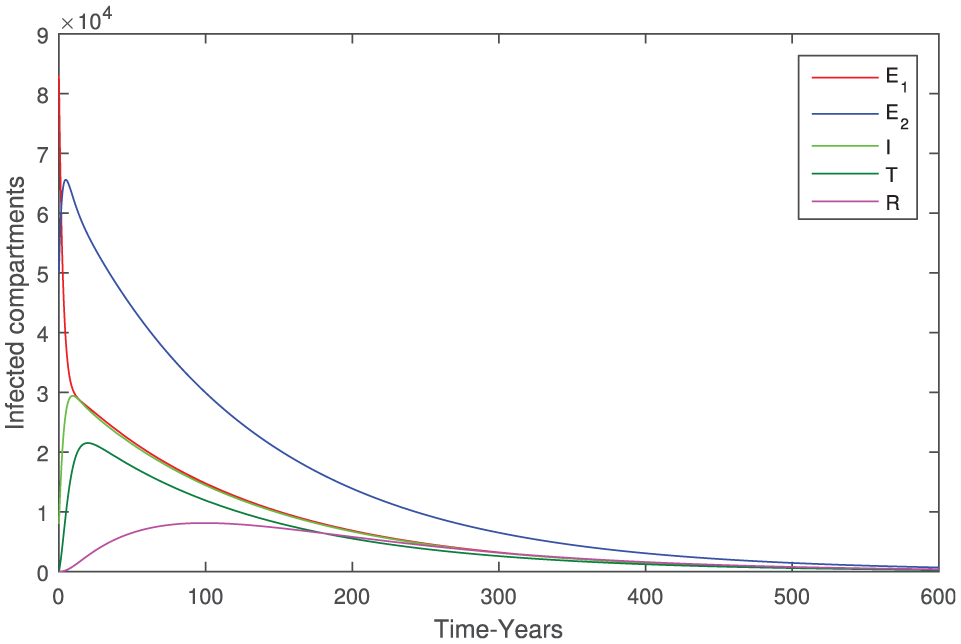
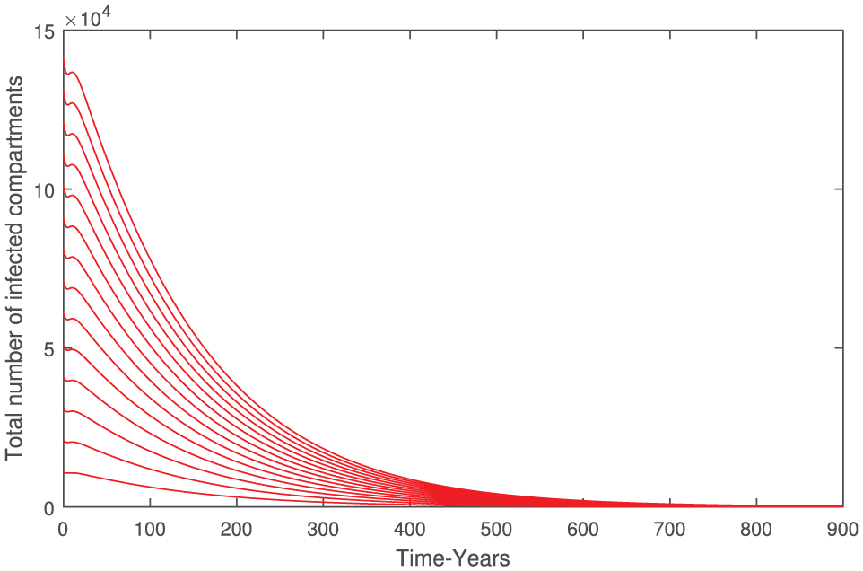
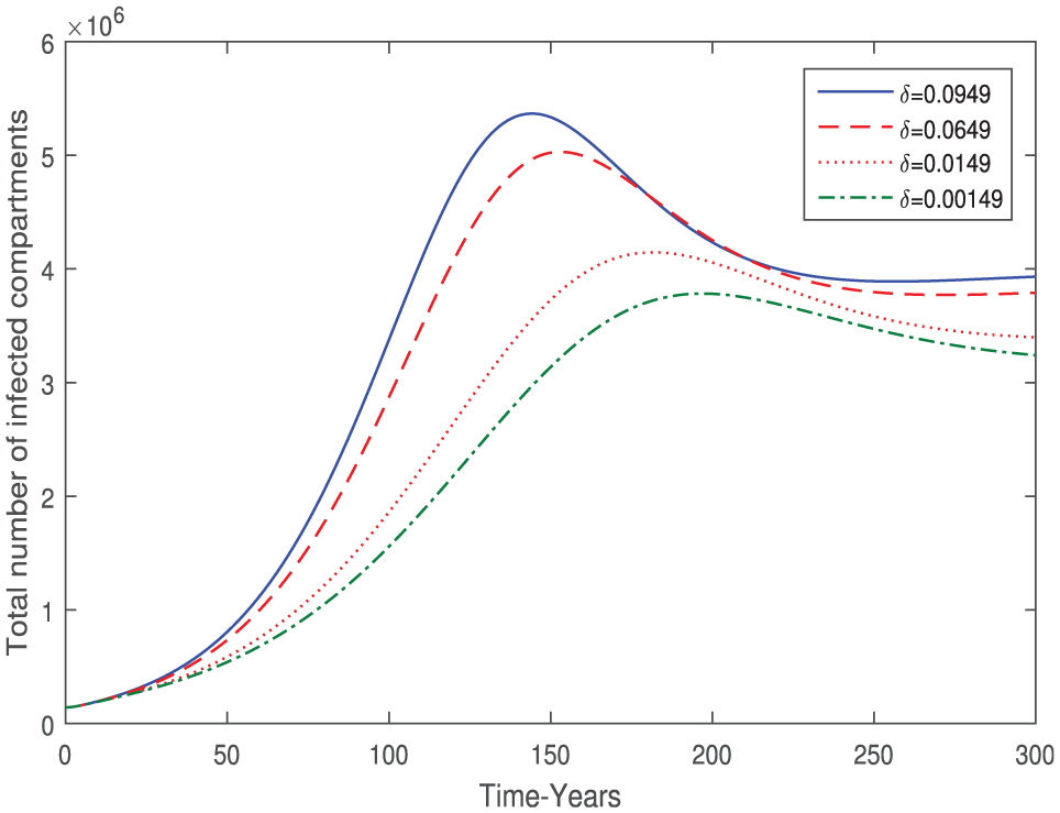
In this section, we simulate the TB model given in equation (2) using the parameter values fitted from field data. These parameter values are given in Table 1. To illustrate the numerical solution of the TB model, we use Software MATLAB and the numerical method is RK4 and present the graphical results. The initial values of the model state variables are taken as follows. It is evident from the source that the Khyber Pakhtunkhwa population as per 2017 was 30,523,371. ⁶ So, we consider this value as the total population, that is, $N(0)=30,523,371$ and assume that the initial population in exposed and infected classes are, respectively, given as $E_1(0)=83,000$ , $E_2(0)=50,000$ , and $I(0)=8010$ . Furthermore, assuming $T(0)=R(0)=0$ as there is no treated or recovered individuals at the initial level. So, the population at the initial level for the susceptible individuals can be obtained as follows: $S(0)=N(0)-E_1(0)-E_2(0)-I(0)-T(0)-R(0)=30,382,361$ . Using these initial values of the system variables and the parameters that are shown in Table 1, we depicted some graphical results. The dynamical behavior of model (2), when ${\mathcal{R}}_0=1.38>1$ and $\beta =0.6001$ is shown in Figure 9, which is an indication that it clearly shows the convergence of the model solution to the proposed EE ${\mathcal{D}}_1$ . Figure 10 depicts the dynamics of model different classes when ${\mathcal{R}}_0=0.9300<1$ and $\beta =0.4001$ . It is clear that in this case all solutions converged to the DFE ${\mathcal{D}}_0$ . Figure 11 shows that all infected classes of model (2) also converged to EE for ${\mathcal{R}}_0=1.38>1$ and taking parameter values given in Table 1. In Figure 12, it is observed by choosing a set of initial values to the model equations the total infected individuals vanishes when ${\mathcal{R}}_0=0.9300$ and $\beta =0.4001$ . In Figure 13, it is shown that when ${\mathcal{R}}_0=1.38>1$ and taking different initial values, the total infected individuals converged to ${\mathcal{D}}_1$ . The effect of treatment is depicted in Figure 14 by taking different values of $\gamma$ . The cumulative number of associated TB infective decreases with increasing of treatment rate $\gamma$ . The effects of the parameters $\delta$ ( leaving rate of treated class by individuals) and $\eta$ are plotted in Figures 15 and 16, respectively. Finally, the model behavior with and without treatment for the infective people whenever ${\mathcal{R}}_0=1.38>1$ and ${\mathcal{R}}_0=0.9300<1$ is shown in Figures 17 and 18, respectively.

Figure 9.

Behavior of the model variables when ${\mathcal{R}}_0=1.38>1$ when $\beta =0.6001$ .

Figure 10.

Behavior of the model variables when ${\mathcal{R}}_0=0.9300<1$ when $\beta =0.4001$ .

Figure 11.

Behavior of the model variables when ${\mathcal{R}}_0=1.38>1$ when $\beta =0.6001$ .

Figure 12.

Dynamical behavior of total number of infected individuals when ${\mathcal{R}}_0=0.9300<1$ and $\beta =0.4001$ .

Figure 13.

Dynamical behavior of total number of infected compartments when ${\mathcal{R}}_0=1.38>1$ and $\beta =0.6001$ .

Figure 14.

Effect $\gamma$ (treatment rate) on the dynamics of the total number of infected individuals.

Figure 15.

Effect of $\delta$ on the dynamics of the total number of infected individuals.

Figure 16.

Effect of $\eta$ on the dynamics of the total number of infected individuals.

Figure 17.

Dynamics of the cumulative infected individuals with and without treatment when ${\mathcal{R}}_0=1.38$ and $\beta =0.6001$ .

Figure 18.

Dynamics of the of cumulative infected individuals with and without treatment when ${\mathcal{R}}_0=0.9300<1$ when $\beta =0.4001$ .

Conclusion

This study is focused on the formulation, analysis, and simulations of a deterministic model for assessing the TB infection dynamics in Khyber Pakhtunkhwa. The model is fitted to the real demographic TB incidence data in Khyber Pakhtunkhwa for the period 2002–2017. The main theoretical and epidemiological findings obtained in this study are summarized below.

1. The biological parameters have been estimated by fitting the model to the real TB incidence data. The RK4 technique has been used to solve the model numerically along with a least-squares optimizer in order to obtain the best fit to field data.

2. Model (2) has a DFE ${\mathcal{D}}_0$ which is GAS if the threshold quantity is ${\mathcal{R}}_0<1$ . Furthermore, it has also a unique EE ${\mathcal{D}}_1$ which is GAS when ${\mathcal{R}}_0>1$ .

3. Using the fitted and estimated parameters, the value of ${\mathcal{R}}_0$ for the described period is ${\mathcal{R}}_0\approx 1.38$ .

4. The sensitivity analysis of the basic reproduction number is performed and the sensitivity indices of various model parameters are obtained. Also, the effect of different important parameters on ${\mathcal{R}}_0$ is shown graphically. Sensitivity results of the model show that the most sensitive parameter is the effective disease transmission coefficient $\beta$ . Furthermore, we conclude that the epidemic of TB can be minimized by decreasing the disease contact rate $\beta$ , treatment failure (incomplete) rate $\eta$ , the proportion $\delta$ , and by increasing the treatment rate $\gamma$ , recovery rate $\alpha$ , and the fraction $q$ .

5. Finally, the numerical simulations of the model are presented to confirm the theoretical results, the impact of treatment on the eradication of TB infection, and to show the effects of important model parameters.

In the near future, based on the sensitivity analysis we will develop the effective time-dependent control model with best strategies for TB eradication in Khyber Pakhtunkhwa.