Sage Journals: Discover world-class research

Abstract

To improve the accuracy of road safety evaluation, this article presents a method to calculate the average crash probability for highway sections based on fault tree and energy method. First, the average crash probability of sections was formulated based on fault tree theory, taking lateral instability, rollover, and rear-end crash into account. Second, an instability factor, which described the extent of steering instability and tire sideslip, was proposed based on energy method. Thereafter, the relationships between the instability factor and probability of lateral instability crash, the load transfer ratio and probability of rollover crash, the available sight distance and probability of rear-end crash were investigated. Then, the driver–vehicle–road multi-body dynamics model was developed based on the three-dimensional alignments of Ning-Luo Expressway using CarSim, the dynamics indexes such as lateral velocity, wheel vertical load were obtained, and the average crash probability of each section was calculated. Finally, the correlation between average crash probability and the average number of accidents was analyzed to validate the accuracy of the proposed method. Results reveal that the proposed method can improve the accuracy of evaluation results, compared with existing methods, thus providing theoretical basis for black spot identification of both design phase and in-service highways.

Keywords

Traffic engineering average crash probability energy method highway alignment fault tree analysis road safety evaluation

Introduction

With the rapid development of highway construction and the continuous growth of car ownership, highway safety has become a widespread concern in China. In 2015, there were 102,281 highway accidents in China, with 40,030 deaths, 111,963 injuries, and 728,335,243 direct economic losses, representing 54.46%, 68.99%, 56.02%, and 70.24% of all road traffic accidents, respectively.¹ Previous studies found that most road traffic accidents occurred on curve sections, longitudinal slope sections, or compound sections. Therefore, road alignment is closely related to traffic accidents.^2,3 With the development of relevant theories and engineering practice, Road Safety Audit has been thought to be an effective means to ensuring road safety throughout the world. Compared with Road Safety Audit of in-service highway, evaluating the safety of highway alignment in design stage and proposing the improvement measures can mitigate the safety risks of highway safety fundamentally and reduce road traffic accidents.

The studies on Road Safety Audit can be divided into the following four categories with a content analysis of relevant papers:

Specialists evaluation based on safety checklists,^4,5 which is defined as “the formal safety performance examination of an existing or future road or intersection by an independent, multidisciplinary team. It qualitatively estimates and reports on potential road safety issues and identifies opportunities for improvements in safety for all road users.” First, the highway safety management department compiles safety checklists based on accident prevention principles, design standards, and highway safety engineering experience. Then specialists analyze the safety risks, searching for deficiencies in road alignment, roadbeds, pavement, bridges, tunnels, and interchanges and propose the improvement measures to highway design plan according to the checklists and their experience. This method is significant for improving highway safety. However, its process and results depend heavily on specialists that makes it hard to promote. Furthermore, it cannot quantitatively evaluate the degree of safety risks, which is unconducive to finding and analyzing key sections with high risks.

Alignment consistency analysis.^6–9 Increased knowledge and experience have proven that a consistent road design that ensures soundly tuned successive elements can produce harmonious and homogeneous driver performance and does not provoke unexpected events. In contrast, inconsistent road designs can produce unexpected changes in the dynamics and speed conditions, which may impose high workloads that can surprise drivers and increase the probability of a crash. It includes design consistency, operating speed consistency, and driving dynamics consistency. Criterion 1 refers to the adjustment of certain elements such that the absolute difference between the design speed V_d and operating speed V₈₅ would remain within certain limits at each element. Criterion 2 requires that the operating speed V₈₅ at adjacent elements remains within certain limits. According to criterion 3, the actual value of side friction, f_R (due to the operating speed) should not be significantly greater than the allowable design value, f_Rd (defined for the design speed). The operating speed model is the key to alignment Consistency analysis. Although there have been many studies on it, it is difficult to establish an accurate and reliable operating speed model when the geometric features of highway are complex. In addition, the indexes of alignment consistency analysis cannot directly reflect the frequency of traffic accidents; thus, the correlation between the results and the actual accidents data is weak (generally under 0.47).¹⁰

Accident prediction model.^11,12 This method establishes the relationship between the number of accidents or accident rate and the parameters such as highway alignment and traffic volume based on accident statistics, and the probability of sections accidents is predicted according to horizontal, longitudinal, and lateral data. It can predict potential accidents in future including the number and the degree of accidents, so that the future safety level of highways can be deduced. Also, it provides quantitative safety analysis tool for road safety evaluation whether in design phase or reconstruction phase. Thus, it has become a favorite topic on recent years with the development of accident data acquisition technology. However, only when this kind of model is applied to highways in specific areas can the prediction accuracy be ideal. When highway characteristics, climate, population and other factors change, they need to be corrected. Studies have shown that the error between the number of predicted accidents and actual accidents after the correction of non-characteristic road sections is still as high as 52.0%–81.2% when adopting the IHSDM model proposed by the US Federal Highway Administration.^13,14

Alignment safety evaluation based on human–vehicle–road system test or simulation.^15,16 This kind of method generally analyzes driver and vehicle response indices (e.g. driver load, steering task interval, tracking error, peak speed of steering wheel, lateral acceleration, vertical load) of different alignment sections via real vehicle test, driving simulator, multi-body dynamics simulation software, vehicle–road coupling mathematical model, and so on, then uses several of these indices or their weighted values to evaluate alignment safety.^17–21 However, such methods are difficult to deal with the relationship between different dynamics indexes, and it is difficult for designers to understand the meaning of these vehicle dynamics indexes, and most studies do not explore the relationship between such indexes and accident risks.

To sum up, specialists evaluation based on safety checklists consumes a lot of resources, and only qualitative analysis can be carried out, and the results are more subjective; the indexes of alignment consistency analysis or alignment safety evaluation based on human–vehicle–road system test or simulation only has a correlation with the frequency of accidents, cannot directly reflect the safety level of highway alignment; accident prediction model can directly predict accident frequency, but it is not accurate.

In fact, it is intuitive and scientific to use risk analysis and accident probability to evaluate the safety of road and highway system.^22–24 In this field, the study of real-time risk prediction and early warning of road traffic system have attracted extensive attention from developed countries in Europe and the United States in recent years, but the study on safety evaluation of static factors (e.g. road design) is relatively scarce. You and colleagues^25–27 have constructed the relationship between the probability of rollover, sideslip, skidding, and the dynamics indexes based on the risk analysis, and the probability of accidents in each section of the highway has been calculated via the fault tree and Monte Carlo method as the safety evaluation results of highway alignment design. However, there is a problem in the definition of accident type (i.e. sideslip is the limit condition of the tire sideslip) and the risk of the rear-end collision is not involved. In addition, previous studies have considered the balance between vehicle centripetal acceleration and lateral adhesion coefficient as the lateral safety boundary. In fact, the steering characteristics also affect the lateral stability, so there is a strong need to establish an accurate index of the lateral safety boundary of the vehicle. Besides, most of the previous studies have classified highway based on geometric alignment,²⁸ which is prone to lead to inconsistencies in length of sections, thereby increasing the heteroscedasticity and the statistical error of the accidents.²⁹ Furthermore, few studies have compared the evaluation results with actual accident data, and the accuracy of the methods needs to be further explored.

Motivated by the above issues, this article aims to develop a safety evaluation method of highway alignment based on fault tree analysis (FTA) and energy method. FTA is a deductive reasoning method that can signify the logic relationships between system possible faults and their causes using a fault tree.³⁰ Through qualitative and quantitative FTA, the major causes of faults are identified, which offer a solid foundation for the accurate calculation of system fault probability and suggest safety countermeasures.³¹ The energy method is used to characterize the vehicles stability. The sum of the lateral motion kinetic energy and the transverse motion energy of the vehicle is defined as the instable kinetic energy; then the ratio of the instable kinetic energy to the longitudinal kinetic energy and the rate of change are established to characterize the vehicle stability.³²

This article is structured as follows: in section “Highway accident probability model based on FTA,” a method for calculating the probability of road accidents that comprehensively considers the rear-end accidents caused by lateral instability, rollover, and inadequate stopping sight distance is developed. In section “Safety index and threshold of accidents,” the instability factor, the index to characterizing the steering and lane-keeping ability of vehicles accurately, is proposed according to the energy method. Then the relationship models between instability factor and lateral instability probability, rate of load transfer and rollover probability, sight distance and rear-end collision probability were presented. In section “Multi-body dynamics simulation of human–vehicle–road system via CarSim,” CarSim is used to construct the multi-body dynamic simulation model of human–vehicle–road system for obtaining dynamics indexes such as lateral velocity, longitudinal velocity, according to the alignment parameters of the sections of Ning-Luo Expressway (G36) between stake number 36000 to stake number 200778. In section “Validation of safety evaluation of highway alignment based on fault tree analysis and energy method,” the fixed-length method is used to divide sections, then the accident probability of each road section is calculated based on the simulation data, and the superiority of the method compared with the traditional fault tree is discussed by comparing the evaluation results with the actual number of accidents. The flowchart of this article is shown in Figure 1.

Figure 1.

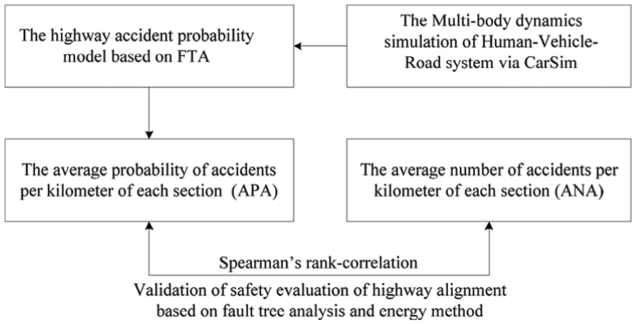
The flowchart of this article.

Highway accident probability model based on FTA

The occurrence of road traffic accidents is a random event. Therefore, it is more direct and accurate to use road accident probability to evaluate road safety relative to driver response indexes and vehicle dynamics response indexes.

Fault tree analysis (FTA) is a system security and reliability analysis method widely used in various fields³³ which can start from the possible faults of the system and gradually find the basic event causing the faults layer by layer, whereby an undesired event (i.e. a traffic crash) is defined, and then the system is analyzed in the context of its environment and operation to find all combinations of basic events that will lead to the occurrence of the predefined undesired event. Also, it can characterize the logical relationship between some kind of faults that may occur in the system and the basic events that cause the fault to occur via the logic tree diagram.³⁴ Through the qualitative and quantitative analysis of the fault tree, the main events leading to system failure can be identified and the probability of system failure can be calculated.

Thus, this article uses FTA to calculate the accident probability of different sections by constructing a fault tree model of highway accident. The primary task of FTA is to categorize the crash types. Since good weather conditions and free traffic flow were assumed in our study.⁸ In such conditions, single-vehicle crashes are caused by lateral instability and rollover.

In addition to the crash types discussed above, the risk of a rear-end crash caused by inadequate stopping sight distance (a vehicle runs into an obstacle or a stopped vehicle) also be considered. Consequently, three failure modes (sub-events) were considered: lateral instability, rollover, and rear-end collision caused by insufficient stopping sight distance. The model structure is shown in Figure 2.

Figure 2.

The fault tree analysis model of highway traffic accidents.

As shown in Figure 1, lateral instability, rollover, and rear-end collision are connected by OR gates; when any of the above-mentioned accidents occurs, the top event (i.e. highway accident) occurs. When the sideslip angle is too large, the car will lose control on lane keeping; when the yaw angular velocity is too small or too large, the car will lose control on steering; both of the above cases will lead to lateral instability. In the current study, instability factor, rate of lateral load transfer, and stopping sight distance are adopted to characterize the lateral stability, the probability of rollover, and rear-end collision, respectively.

According to the OR gate algorithm in the FTA model, the probability of an accident in a certain position of the section is as follows

P (s) = 1 - Π_{i = 1}^{3} [1 - P_{i} (s)]

(1)

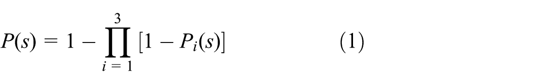
where P(s) is the probability of accident at station s, and P_i(s) is the probability of the i accident at station s, which can be obtained by

P_{i} (s) = {\begin{matrix} \frac{| I_{i} (s) |}{I_{i}^{0}} | I_{i} (s) | \leq I_{i}^{0} \\ 1 | I_{i} (s) | > I_{i}^{0} \end{matrix}

(2)

where I_i(s) indicates the risk index of type i accident at station s, and $I_{i}^{0}$ is the safety threshold of the risk index of type i accident at station s.

According to equations (1) and (2), the average accident probability P_n per unit distance of section n is

P_{n} = \frac{1}{d_{n}} \int_{s_{n - 1}}^{s_{n}} P (s) ds

(3)

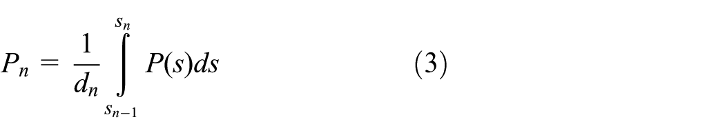
where $s_{n - 1}$ and s_n are station numbers of starting point and ending point of section n, and d_n is the length of the section

d_{n} = s_{n} - s_{n - 1}

(4)

Safety index and threshold of accidents

In order to get P_n, it is necessary to construct appropriate risk indexes and calculate the safety boundary of risk index for lateral instability, rollover, and rear-end collision, respectively.

Evaluation index of lateral instability based on energy method

The balance between lateral force coefficient and lateral adhesion coefficient is generally used to characterize the extreme condition of lateral stability of the vehicle in highway design.³⁵ However, there are at least three disadvantages to this index. First, the lateral adhesion coefficient is affected by the longitudinal acceleration/deceleration, and the vertical/cross-section alignment; also it is constrained by friction ellipse, so the accuracy of estimation formula is low. Second, since the tire is elastic, its sideslip characteristics make the vehicle lose control on lane keeping before full sideslip, so the safety boundary determined by this index is conservative. Third, it is unable to characterize steering stability of vehicle.

Motivated by the above problems, a new instability factor k_s is defined to accurately characterize the degree of steering instability/sideslip based on the energy method.

The total kinetic energy of the vehicle during driving can be divided into the front axle kinetic energy E_Tf and the rear axle kinetic energy E_Tr,³⁶ as shown in equations (5) and (6)

E_{Tf} = \frac{1}{2} m_{f} (u_{f}^{2} + v_{f}^{2}) + \frac{1}{2} I_{zf} ω_{r}^{2}

(5)

E_{Tr} = \frac{1}{2} m_{r} (u_{r}^{2} + v_{r}^{2}) + \frac{1}{2} I_{zr} ω_{r}^{2}

(6)

u_{f} = u_{r} = u

(7)

v_{f} = v + l_{f} ω_{r}

(8)

v_{r} = v - l_{r} ω_{r}

(9)

where m_f and m_r are equivalent to the mass of the front of (to the front axle) and the rear of (to the rear axle) the vehicle, respectively. I_zf and I_zr are the rotational inertia of the front and rear of the vehicle around thez-axis, respectively. u, u_f, u_r are the longitudinal speed of the vehicle and the longitudinal speed of the front and rear wheels, respectively. v, v_f, v_r are the lateral speed of the vehicle and the lateral speed of the front and rear wheels, respectively. $ω_{r}$ is yaw angular velocity. l_f and l_r are the horizontal projection distances from the centroid to the front and rear axle, respectively.

The longitudinal kinetic energy of the vehicle E₁ is as follows

E_{1} = \frac{1}{2} (m_{f} + m_{r}) u^{2}

(10)

The lateral instability kinetic energy of the vehicle E₂ is as follows

E_{2} = \frac{1}{2} (m_{f} + m_{r}) v^{2} + \frac{1}{2} I_{z} ω_{r}^{2}

(11)

The lateral instability energy ratio R to measure the lateral instability of the vehicle is as follows³²

R = \frac{E_{2}}{E_{1}} = \frac{(m_{f} + m_{r}) v^{2} + I_{z} ω_{r}^{2}}{(m_{f} + m_{r}) u^{2}} \approx \frac{v^{2}}{u^{2}}

(12)

In order to obtain the range of R before lateral instability, phase plane method (i.e. the instability energy ratio is taken as the abscissa, and the instability energy ratio change rate is taken as the ordinate) can be used for analysis.³⁷ In this phase plane, we can find a stable region in which the phase trajectory from any initial point finally converges to a stable focus (saddle point), that is, the vehicle can return to the corresponding stable state. According to the Testing Method for Vehicle Handling Stability (GB/T 6323-2014), the steering wheel angle step input test and the serpentine test are carried out in CarSim to simulate critical conditions of vehicle under rapid steering and continuous obstacle avoidance, respectively. In order to investigate the instability, the road adhesion coefficient ranges from 0.2 to 0.8.

An improved diamond stable region partition method with five-eigenvalue³⁸ is adopted. According to the changing of phase diagram, the diamond region moving with equilibrium point is selected as the stable region, and the boundary of the stable region is defined by the following formula³²

k_{s} = | C_{1} R + C_{2} \overset{\cdot}{R} |

(13)

where k_s is the instability factor of vehicle lateral stability index. According to the boundary of the diamond region, it is found that C₁ = 18.5, C₂ = 5.6. When k_s is 1, lateral instability occurs.

Rollover evaluation index

The mechanism of rollover is complicated, and its common indexes include load transfer ratio (LTR), time to rollover (TTR), and so on.³⁹ LTR is simple and positively correlated with rollover risk. Therefore, it is adopted as rollover index in the current study^40–42

LTR (s) = \sum_{i = 1}^{i = 2} | \frac{F_{ZR} {(s)}_{i} - F_{ZL} {(s)}_{i}}{F_{ZR} {(s)}_{i} + F_{ZL} {(s)}_{i}} |

(14)

where LTR(s) denotes the load transfer rate at station s, F_ZR(s)_i denotes the vertical load on the right wheel (N); F_ZL(s)_i is the vertical load of the left wheel (N); i = 1 means the front wheel; i = 2 means the rear wheel. The security threshold of LTR(s) is 1.

Rear-end collision evaluation index

If there is an obstacle in front during driving, the road needs to provide sufficient stopping sight distance; otherwise, a rear-end collision will occur. The following formula is defined as an evaluation index of the rear-end collision

{\begin{matrix} r_{s} = \frac{SSD (s)}{R_{ASD} (s)} R_{ASD} (s) > SSD (s) \\ r_{s} = 1 R_{ASD} (s) \leq SSD (s) \end{matrix}

(15)

where r_s denotes the risk index of rear-end collision with a threshold of 1, R_ASD(s) denotes the available sight distance at the station s (m), SSD(s) denotes the stopping sight distance required for safety (m) which is calculated by the following formula⁴³

SSD (s) = 0.278 Vt + \frac{V^{2}}{254 (\frac{a}{9.81} \pm i)}

(16)

where V denotes the initial speed of braking (km/h), t denotes the driver response time and the value is 2.5 s, i denotes slope, and a denotes braking deceleration and the value is 3.4 m/s².

The available sight distance on section is limited by obstacles on horizontal curve (e.g. central dividers, green belts, and bridge abutment), vertical alignments (e.g. the obstruction of crest vertical curve to sight, the restriction of sag vertical curve on headlamp illumination distance at night), and upper limit of driver’s visual field. The available sight distance is the minimum of the three, and the upper limit of the driver’s sight distance is 400 m.⁴⁴

Available sight distance on horizontal curve

When there are buildings, trees, guardrails, or other artificial structures in the inside of the horizontal curve, it is prone to obstruct the driver’s sight. Meanwhile, when driving in the outer lane with central dividers, anti-collision guardrails, green belts, or anti-glare vision protection will also obstruct sight, resulting in inadequate stopping sight distance and causing traffic accidents. The available sight distance on horizontal curve is calculated by the following formula⁴⁵

H_{ASD} = 2 R_{h} \arccos (1 - \frac{W_{l} / 2 + W_{c}}{R_{h}})

(17)

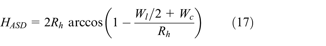
where H_ASD denotes the available sight distance on horizontal curve (m), W_l denotes lane width (m), W_c denotes lateral clearance (m), and R_h denotes radius of horizontal curve (m).

When the vehicle turns right, roadside guardrails and green belts will obstruct the driver’s sight; while when turning left, central dividers and guardrails will obstruct the driver’s sight. By considering this point, lateral clearance is calculated by the following formula

W_{c} = {\begin{matrix} W_{s} - W_{b} / 2 when turning right \\ (W_{m} - W_{b}) / 2 when turning left \end{matrix}

(18)

where W_s denotes shoulder width (m), W_b denotes guardrail width (m), and W_m denotes the width of central divider (m).

Available sight distance on crest vertical curve

When driving on a crest vertical curve, the sight distance will be affected by the minimum radius of the crest vertical curve. Thus, appropriate radius of vertical curve must be adopted in design phase to ensure the requirement of stopping sight distance. Assume that the height of driver’s eyes is h₁ and the height of the observed object is x. The illustration for calculating available sight distance of crest vertical curves is shown in Figure 3, and the formulas are as follows⁴⁶

T_{ASD} = (α_{1} + α_{2}) R_{v}

(19)

α_{1} = \arccos (\frac{R_{v}}{h_{1} + R_{v}})

(20)

α_{2} = \arccos (\frac{R_{v}}{x + R_{v}})

(21)

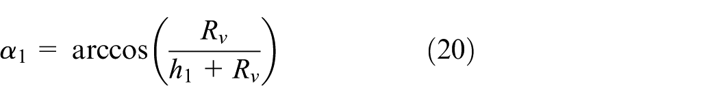
where T_ASD denotes the available sight distance on crest vertical curve (m), R_v denotes radius of crest vertical curve (m), h₁ takes on the value of 1.08 m,⁴³ and x takes on the value of 0.6 m.⁴³

Figure 3.

Illustration for calculating the available sight distance of crest vertical curves.

Available sight distance on sag vertical curve

The sag vertical curve needs to ensure that the headlamp illumination distance is adequate at night. The illustration for calculating available sight distance of sag vertical curves is shown in Figure 4, and the formulas are as follows⁴⁶

S_{ASD} = (α_{3} + α_{4}) R_{S}

(22)

α_{3} = β

(23)

α_{4} = \arccos (\frac{OE}{R_{S} - x})

(24)

OE = (R_{S} - h_{2}) \cos (α_{3})

(25)

where S_ASD denotes the available sight distance on sag vertical curve (m), R_s denotes radius of sag vertical curve (m), β denotes diffusion angle upward for headlamp, the maximum is 1.5°,⁴² and h₂ denotes the height of headlamp⁴⁴ with the value of 0.6 m.⁴³

Figure 4.

Illustration for calculating the available sight distance of sag vertical curves.

Multi-body dynamics simulation of human–vehicle–road system via CarSim

CarSim is a professional simulation software for automobile system developed by MSC (Mechanical Simulation Corporation). Since more than 20 years, its model has undergone a lot of experiments, and CarSim has been widely used by many automobile manufacturers and parts suppliers worldwide. In addition to vehicle dynamics analysis, CarSim has also been widely used in road safety design and evaluation.^47,48

The human–vehicle–road multi-body dynamics model is developed based on the three-dimensional alignments of Bengbu to Nanjing section of Ning-Luo Expressway (G36) by CarSim, and the dynamics indexes such as lateral velocity, longitudinal velocity, wheel vertical load are obtained. Integrated with the design data, including horizontal curve radius, vertical curve radius, slope, and so on collected from AutoCAD files, were input into the highway accident probability model based on fault tree analysis, then the accident probability per unit distance of each section upstream and downstream is calculated and the average of whom is taken as the accident probability per unit distance of the section, which is used to evaluate the highway alignment safety.

After setting the simple parameters input in CarSim, it will model the different modules of vehicle, driver control, and highway and finally derive the complex multi-body dynamics simulation model of human–vehicle–road.

Highway module

The human–vehicle–road multi-body dynamics model is developed based on the three-dimensional alignments of Bengbu to Nanjing section of Ning-Luo Expressway by CarSim for safety evaluation. The total length of the section between station 36000 and station 200778 is 164.778 km, the minimum radius of horizontal curve is 5500 m, and the maximum slope is 3%. The section between station 48700 and station 200778 is two-way and two-lane, subgrade width is 28 m, and pavement width is 23.5 m. The design speed of the whole road is 120 km/h, the shoulder width of the dirt road is 0.75 m, the shoulder of the right side is 3 m, the lane width is 3.75 m, the width of central divider is 3 m, and the guardrail width is 1 m.

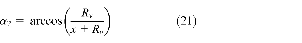
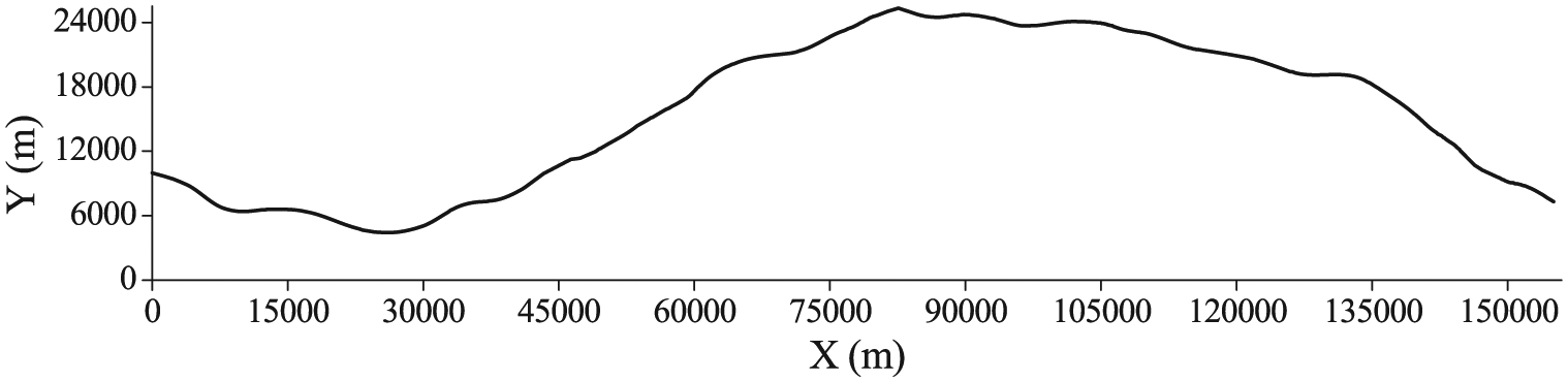
The horizontal and vertical alignments of Beng-Ning section on G36 Expressway are shown in Figures 5 and 6. In Figure 5, the x-y coordinate represents the relative position of the horizontal alignments of Beng-Ning section of G36. In Figure 6, the x-coordinate is the stake number, and the y-coordinate is the elevation of the road centerline. The highway model is established and modified via CarSim its own 3D highway model. According to the AutoCAD files, the horizontal coordinate and the vertical coordinate of the road centerline are extracted, then input them into the highway horizontal module (centerline geometry: Horizontal(X-Y) table) and the highway vertical module (centerline elevation: Z vs S), respectively. Then “Constant: 0.75” in the submenu of the highway friction coefficient module is selected, which means that the pavement adhesion coefficient is set to 0.75. Thereby, the highway model is constructed completely.

Figure 5.

The horizontal alignments of Beng-Ning section of G36.

Figure 6.

The vertical alignments of Beng-Ning section of G36.

Vehicle module

Vehicle model can be customized in CarSim, which is solved by appropriate abstraction of the full-vehicle model, combination with modern multi-body dynamics and traditional vehicle dynamics modeling, simulation initial conditions, and vehicle characteristic parameters. CarSim’s full-vehicle model includes the following seven subsystems: body, aerodynamics, transmission system, brake system, steering system, tire, and suspension system. The E class car in CarSim is chosen as the representative^49,50 in the current study; the main parameters are shown in Table 1.

Table 1.

The main parameters of automobile model.

Parameters	Value
Length (mm)	4350
Width (mm)	1880
Height (mm)	1550
Sprung mass (kg)	1653
Unsprung mass (kg)	180
Wheel base (mm)	1600
Roll angular momentum (kg m²)	614
Pitch angular momentum (kg m²)	2765
Yaw angular momentum (kg m²)	2765
Barycentre to front axle distance (mm)	1402
Barycentre to rear axle distance (mm)	1646
Barycentre height (mm)	590

Driver control module

The driver control model includes direction control and speed control. Direction control is set to preview and track the vehicle trajectory along the centerline of the lane and “Steering: Drive path follower” is selected in the direction control module. Vehicle operating speed is v85 and calculated according to the Calculation Method of Operating Speed in Safety Evaluation Criterion for Highway Projects (JTG B05-2015). The speed control model can be constructed by inputting the speed that changes over stations into speed control module (Target speed vs station) in CarSim.

Validation of safety evaluation of highway alignment based on fault tree analysis and energy method

Accident data were collected from the road crash information system maintained by the Anhui provincial traffic police. From December 2005 to February 2017, there were 322 traffic accidents in the Bengbu to Nanjing section of Ning-Luo Expressway (G36), including 185 rear-end accidents, 109 collisions with fixed objects and stationary vehicles, 14 collisions with non-fixed objects, 13 rollover accidents, and 1 crash accident. These accidents resulted in 220 deaths and 354 injuries. However, it should be noted that the number of crashes may be underreported because some property-damage-only crashes were reported to insurance companies rather than to traffic police. By analyzing the correlation between the average number of accidents (ANA) per kilometer of each section and the average probability of accidents (APA) per kilometer of each section, the accuracy of the evaluation results can be verified.

At present, there are two most widely used methods for dividing road sections in highway safety evaluation:⁵¹ one is fixed-length method in which the road is divided into equal length sections; and the other is homogeneity method in which the section with the same geometric features is divided into one section. Shankar et al.⁵² found that the homogeneity method is prone to the following problems: (1) due to excessive number of sections with different horizontal curve radii and slopes, the number of divided sections is increased, and the length of some sections is less than 1 km. However, the station recorded in the accident database is the station number closest to the accident point. Therefore, this method is prone to increasing the accident statistical error. (2) The length of the section based on the homogeneity method will increase the potential heteroscedasticity. The fixed-length method is simple and can effectively overcome the above disadvantages of the homogeneity method. Therefore, the fixed-length method is performed in the current study. The total length of 164.778 km road is divided into 33 sections and 17 sections by 5 and 10 km, respectively (the last section with a length less than 5 or 10 km is reserved).

In order to explore the superiority of the proposed method, the results of the proposed method are compared with those of the traditional fault tree analysis. The traditional fault tree analysis method divides the accident into three types: rollover, sideslip and skidding, and the balance between the vehicle centripetal acceleration and the lateral adhesion coefficient are used as the sideslip safety boundary.²⁵

The calculation results of the two methods and the average number of accidents per unit distance under the conditions of dividing the sections with 5 and 10 km are shown in Tables 2 and 3.

Table 2.

The APA calculated by two methods and the ANA (dividing the sections with 5 km).

Section ID	APA by method 1	APA by method 2	ANA	Section ID	APA by method 1	APA by method 2	ANA
1	0.748	0.040	2.80	18	0.725	0.122	2.20
2	0.733	0.065	2.00	19	0.748	0.060	3.40
3	0.734	0.037	1.80	20	0.734	0.037	2.80
4	0.718	0.032	1.60	21	0.723	0.046	2.40
5	0.715	0.027	1.20	22	0.707	0.024	1.00
6	0.725	0.043	1.60	23	0.738	0.046	2.40
7	0.727	0.050	1.80	24	0.707	0.029	2.20
8	0.740	0.054	2.60	25	0.710	0.018	1.40
9	0.715	0.036	1.20	26	0.709	0.020	1.00
10	0.732	0.071	1.60	27	0.699	0.034	1.20
11	0.737	0.075	2.80	28	0.733	0.046	1.80
12	0.739	0.023	2.80	29	0.712	0.030	.80
13	0.726	0.043	1.60	30	0.712	0.038	1.00
14	0.752	0.049	3.00	31	0.724	0.055	1.80
15	0.735	0.033	2.40	32	0.721	0.097	2.20
16	0.716	0.051	2.00	33	0.715	0.044	1.26
17	0.730	0.057	2.80^a

APA: average probability of accidents; ANA: average number of accidents.

The APA calculation method based on fault tree and energy method proposed in this article is method 1; the APA calculation method based on traditional fault tree analysis is method 2.

Table 3.

The APA calculated by two methods and the ANA (dividing the sections with 10 km).

Section ID	APA by method 1	APA by method 2	ANA	Section ID	APA by method 1	APA by method 2	ANA
1	0.740	0.055	2.40	10	0.741	0.050	3.10
2	0.726	0.035	1.70	11	0.715	0.035	1.70
3	0.720	0.035	1.40	12	0.723	0.040	2.30
4	0.734	0.050	2.20	13	0.709	0.020	1.20
5	0.724	0.055	1.40	14	0.716	0.040	1.50
6	0.738	0.045	2.80	15	0.712	0.035	.90
7	0.739	0.045	2.30	16	0.722	0.075	2.00
8	0.726	0.040	2.20	17	0.715	0.044	1.26
9	0.728	0.090	2.50

APA: average probability of accidents; ANA: average number of accidents.

In Tables 2 and 3, the APA calculated by method 2 ranged from 0.01 to 0.12, and the APA of all sections is small, which is difficult to identify dangerous sections.

Spearman’s rank correlation was used to determine the level of agreement between the average probability of accidents (APA) of each section and the average number of accidents (ANA) per kilometer. Spearman’s correlation coefficient is a non-parametric statistical method that does not require the distribution of original variables, which can describe the degree of correlation between two variables.⁵³ Spearman’s test is performed on the APA calculated by the two methods and the ANA.

Comparisons between the results obtained in this article and those obtained in previous works were also made to assess the effectiveness of the proposed method. Particular attention should be paid to the method of You et al.,²⁵ as it is similar to the method proposed here. The main differences between the two methods are that in their study, rollover, sideslip, and tire cornering are considered as the failure modes in FTA, and the dynamic characteristics of the safety boundaries were not fully considered. The method of You et al.²⁵ was implemented on the expressway in our study, and the safety evaluation results were derived. The test results of the different methods are shown in Table 4.

Table 4.

Comparisons of different methods.

	Dividing the sections with 5 km		Dividing the sections with 10 km
	Method 1	Method 2	Method 1	Method 2
Spearman correlation coefficient	0.806	0.474	0.871	0.588
Sig. (two-sided)	0.000	0.005	0.000	0.013
N	33	33	17	17

Table 4 shows that Spearman’s correlation coefficients of the APA and the ANA based on fault tree and energy method are 0.806 and 0.871, respectively, under the conditions of dividing the sections with 5 and 10 km, which are better than those of the traditional fault tree method (0.474 and 0.588). Thus, the accuracy of the proposed safety evaluation of highway alignment is higher. In addition, for the two methods, the correlation coefficient between the evaluation results and the ANA decreases with the decreasing of the average length of the divided sections. The main reason is that the number of accident samples collected in this article is relatively small, and the random error increases with the decrease of the ANA. Large sample data can be analyzed in future study to verify the proposed method further.

Conclusion

The main innovations of this study include (1) a fault tree model of highway traffic accidents considering lateral instability, rollover, and rear-end collision is proposed, which can reflect the types of highway traffic accidents more comprehensively. (2) Taking the balance of vehicle centripetal acceleration and lateral adhesion coefficient as the lateral safety boundary, the index estimation formula has low accuracy, the boundary value is too conservative, and it cannot reflect the steering stability of the vehicle. Based on the energy method, the instability factor which can accurately characterize the steering stability and track keeping ability of automobiles is proposed in this study. (3) The proposed method was implemented on the expressway from Bengbu to Nanjing. Results of statistical tests against crash data collected from the road revealed that the proposed method outperforms the methods used in previous studies in terms of accuracy.

The proposed method has the potential to be used in practical engineering applications to identify crash-prone locations (black spot) and alignment deficiencies for on highways in the planning and design phases, as well as those in -service. With the result, those hazardous road sections associated with high average crash probabilities would be identified. Then, safety facilities, such as speed limit signs, sight guidance facilities, and anti-skid pavement sheeting, are suggested to improve the safety performances of these sections. However, in particular, the aim of the paper is only to evaluate safety performance of highway alignments; the other structural characteristics of the highways, apart from the geometric alignment, like the structural and physical features of road infrastructure and environment (bridges, tunnels, mountains, hills), would be considered in the further research.

This study mainly explores the risk of rear-end collision caused by lateral instability, rollover, and inadequate stopping sight under the condition of good weather and free flow. When the vehicle is in a free-flow state, the traffic flow density is low, the vehicles do not interfere with each other, and the complicated alignment sections are prone to the above types of accidents. However, under the condition of synchronized flow and wide moving jam, the degree of driving freedom decreases. Meanwhile, the behavior of vehicle is mainly following and changing lanes. Frequent braking/starting can easily lead to rear-end accidents in sections with large longitudinal slope, which is not caused by inadequate stopping sight distance. In addition, cross-sectional design parameters such as lane width, number of lanes, and central dividers width have a significant effect on lane changing behavior, which in turn affects the probability of lateral collision accidents. Therefore, studying the coupling mechanism between dynamic factors (e.g. traffic flow, weather) and geometric alignment in highway traffic accidents is the key to further improving the accuracy and scientificity of highway alignment safety evaluation, and it is also one of the important tasks that this article needs to carry out in the future. In addition, the impact of drivers’ driving behaviors on highway alignment safety will also be considered.⁵⁴

Footnotes

Handling Editor: Yanyong Guo

Declaration of conflicting interests

The author(s) declared no potential conflicts of interest with respect to the research, authorship, and/or publication of this article.

Funding

The author(s) received no financial support for the research, authorship, and/or publication of this article.

ORCID iD

Zhijian Chen

References

National Bureau of Statistics of China. Road traffic accident statistics annual report in 2015 of People’s Republic of China. 1st ed. Beijing, China: China Statistics Press, 2016, pp.154–196.

Eftekharzadeh

Khodabakhshi

. Safety evaluation of highway geometric design criteria in horizontal curves at downgrades. Int J Civil Eng 2014; 12: 326–332.

Kang

Shariat

Jha

. New highway geometric design methods for minimizing vehicular fuel consumption and improving safety. Transp Res Part C Emerg Technol 2013; 31: 99–111.

Lougheed

Hildebrand

. Road safety audits and major P-3 freeway projects: quantifying the findings. Can Int J Civ Eng 2015; 42: 1083–1090.

Zhong

Liu

Chen

et al . Questionnaire survey of highway safety audit management policy. In: International conference of transportation professionals, Beijing, China, 3–6 August 2012. Reston, VA: ASCE.

Dell’Acqua

Russo

. Road performance evaluation using geometric consistency and pavement distress data. Transp Res Rec J Transp Res Board 2011; 2203: 194–202.

Sheng

. Research on highway safety design theory based on alignments design consistency. PhD Thesis, Beijing Jiaotong University, Beijing, China, 2014.

Cvitanic

Vukoje

Breški

. Methods for ensuring consistency of horizontal alignment elements. Građev 2012; 64: 385–393.

Pratico

Giunta

. Quantifying the effect of present, past and oncoming alignment on the operating speeds of a two-lane rural road. Baltic J Road Bridge Eng 2012; 7: 181–190.

10.

Cafiso

Cava

. Driving performance, alignment consistency, and road safety: real-world experiment. Transp Res Rec J Transp Res Board 2009; 2102: 1–8.

11.

Mun

. Design speed based reliability index model for roadway safety evaluation. KSCE J Civil Eng 2012; 16: 845–854.

12.

Meng

Hou

Shi

. Research on accident prediction models for freeways in mountainous and rolling areas. In: Proceedings of the measuring technology and mechatronics automation, Nanchang, China, 13–14 June 2015. New York: IEEE.

13.

Donnell

Gross

Stodart

et al . Appraisal of the interactive highway safety design model’s crash prediction and design consistency modules: case studies from Pennsylvania. J Transp Eng 2009; 135: 62–73.

14.

Meng

Zhang

Zheng

. Prediction of rear-end collision on mountainous expressway based on geometric alignment and traffic conditions. China J Highw Transp 2012; 25: 113–118.

15.

Ren

. Safety evaluation of road alignment based on human-vehicle-road virtual test. Highway 2011; 9: 171–175.

16.

Jiang

. Research on highway geometric alignment evaluation criteria based on vehicle dynamic simulation. Master Thesis, Southeast University, Nanjing, China, 2013.

17.

Shao

Yang

et al . Analysis of adaptability of large vehicles on mountainous highways based on driver-vehicle-road collaborative simulation. China J Highw Transp 2015; 28: 14–25.

18.

Yang

Zhang

. Safety evaluation method of combination of vertical and horizontal curves for mountainous expressway. China J Highw Transp 2010; 2010: 89–92.

19.

. Geometric design safety estimation based on tire–road side friction. Transp Res Part C Emerg Technol 2016; 63: 114–125.

20.

Shu

Shao

. Effects of geometric features of highway horizontal alignment on steering behavior of passenger car. J Vibro Eng 2016; 18: 4086–4104.

21.

Mavromatis

Psarianos

. Investigation of vehicle motion on sharp horizontal curves combined with steep longitudinal grades. Transport Lett 2016; 8: 220–228.

22.

Sun

. A dynamic Bayesian network model for real-time crash prediction using traffic speed conditions data. Transport Res Part C Emerg Tech 2015; 54: 176–186.

23.

Wang

Liu

et al . Analysis of crash risks by collision type at freeway diverge area using multivariate modeling technique. J Transp Eng 2015; 141: 04015002.

24.

Abdel-Aty

. Utilizing support vector machine in real-time crash risk evaluation. Accid Anal Prev 2013; 51: 252.

25.

You

Sun

. Risk analysis-based identification of road hazard locations using vehicle dynamic simulation. J Southeast Univ 2012; 42: 150–155.

26.

You

Sun

. Reliability-based risk analysis of roadway horizontal curves. J Transp Eng 2012; 138: 1071–1081.

27.

You

Sun

. Reliability analysis of vehicle stability on combined horizontal and vertical alignments: driving safety perspective. J Transp Eng 2013; 139: 804–813.

28.

The Ministry of Transportation of the People’s Republic of China. Specifications for highway safety audit: JTG B05-2015. Beijing, China: China Communication Press, 2016.

29.

Zhong

Chen

Sun

et al . Research on section division of freeway with ordinal clustering method. J Wuhan Univ Tech 2008; 32: 43–46.

30.

Miao

Yang

Liang

. Pedestrian crash risk assessment and intervention. Adv Mech Eng. Epub ahead of print 4 July 2016. DOI: 10.1177/1687814016653296

31.

Bas

. A framework for child safety and health management by analogy to occupational safety and health management. Safety Sci 2014; 64: 1–12.

32.

Luo

Lai

. A research on vehicle stability judgment based on energy method. Automot Eng 2014; 12: 1534–1538.

33.

Misra

. Handbook of performability engineering. London: Springer, 2008.

34.

Volkanovski

Čepin

Mavko

. Application of the fault tree analysis for assessment of power system reliability. Reliabil Eng Syst Safety 2009; 94: 1116–1127.

35.

Yang

. Road survey and design. 3rd ed. Beijing, China: China Communications Press, 2013.

36.

Lin

. Vehicle system dynamics. Beijing, China: China Machine Press, 2015.

37.

Liu

Chen

. Vehicle stability control based on phase plane method. Chin J Eng Design 2014; 12: 1534–1538.

38.

Liu

Xiong

Deng

et al . Vehicle stability criterion based on phase plane method. J South China Univ Tech 2014; 42: 63–70.

39.

Chu

. A research on anti-rollover control for vehicles with semi-active suspension. Automot Eng 2012; 34: 399–402.

40.

Rath

Defoort

Veluvolu

. Rollover index estimation in the presence of sensor faults, unknown inputs, and uncertainties. IEEE Trans Intel Transport Syst 2016; 17: 2949–2959.

41.

Tsourapas

Piyabongkarn

Williams

et al . New method of identifying real-time predictive lateral load transfer ratio for rollover prevention systems. In: American control conference, St. Louis, MO, 10–12 June 2009, pp.439–444. New York: IEEE Press.

42.

Larish

Piyabongkarn

Tsourapas

et al . A new predictive lateral load transfer ratio for rollover prevention systems. IEEE Trans Vehic Tech 2013; 62: 2928–2936.

43.

American Association of State Highway and Transportation Officials. A policy on geometric design of highways and streets. Washington, DC: American Association of State Highway and Transportation Officials, 2011.

44.

Liao

Shao

et al . Calculation and assessment technique of highway 3D dynamic sight distance. J Jilin Univ 2013; 43: 640–645.

45.

Sun

You

. Reliability-based risk analysis of vehicle moving on curved sections considering multiple failure modes. China J Highw Transp 2013; 26: 36–42.

46.

Nie

Zhao

. The inspection of stopping sight distance for highway in China and France. Highway 2008; 9: 62–66.

47.

Stine

Hamblin

Brennan

et al . Analyzing the influence of median cross-section design on highway safety using vehicle dynamics simulations. Accid Anal Prev 2010; 42: 1769.

48.

Zhang

Meng

Wang

. Sideslip risk simulation analysis of passenger car braking behavior on expressway curved sections. China J Highw Transp 2015; 28: 134–142.

49.

Kordani

Molan

. The effect of combined horizontal curve and longitudinal grade on side friction factors. KSCE J Civil Eng 2015; 19: 303–310.

50.

Brown

Brennan

. On the required complexity of vehicle dynamic models for use in simulation-based highway design. J Safety Res 2014; 49: 105–112.

51.

Miaou

Wright

et al . Development of relationship between truck accidents and geometric design: phase I. Final report. Mathematical Models, 1993, https://trid.trb.org/view/374727

52.

Shankar

Mannering

Barfield

. Effect of roadway geometrics and environmental factors on rural freeway accident frequencies. Accid Anal Prev 1995; 27: 371–389.

53.

Cafiso

Cava

. Safety index for evaluation of two-lane rural highways. Transport Res Record J Transp Res Board 2007; 2019: 136–145.

54.

Hao

Xiang

et al . The impact of aggressive driving behavior on driver-injury severity at highway-rail grade crossings accidents. J Adv Transp 2018; 2018: 9841498.

Evaluating safety performance of highway alignment utilizing fault tree analysis and energy method

Abstract

Keywords

Introduction

Highway accident probability model based on FTA

Safety index and threshold of accidents

Evaluation index of lateral instability based on energy method

Rollover evaluation index

Rear-end collision evaluation index

Available sight distance on horizontal curve

Available sight distance on crest vertical curve

Available sight distance on sag vertical curve

Multi-body dynamics simulation of human–vehicle–road system via CarSim

Highway module

Vehicle module

Driver control module

Validation of safety evaluation of highway alignment based on fault tree analysis and energy method

Conclusion

Footnotes

Declaration of conflicting interests

Funding

ORCID iD

References